The Diffuse Gamma-Ray Background from Supernovae

Abstract

The diffuse extragalactic $\gamma$-ray background in the MeV region is believed to be due to photons from radioactivity produced in supernovae throughout the history of galaxies in the universe. In particular, $\gamma$-ray line emission from the decay chain ${}^{56}{\rm Ni}\rightarrow$ ${}^{56}{\rm Co}\rightarrow$ ${}^{56}{\rm Fe}$ provides the dominant photon source (Clayton & Silk (1969)). Although iron synthesis occurs in all types of supernovae, the contribution to the background is dominated by Type Ia events due to their higher photon escape probabilities. Estimates of the star formation history in the universe suggest a rapid increase by a factor $\sim$ 10 from the present to a redshift z_p $\sim$ 1.5, beyond which it either remains constant or decreases slowly. Little is known about the cosmological star formation history for redshift exceeding z $\sim$ 5. We integrate the observed star formation history to determine the Cosmic Gamma-Ray Background (CGB) from the corresponding supernova rate history. In addition to $\gamma$-rays from short-lived radioactivity in SNIa and SNII/Ib/Ic we also calculate the minor contributions from long-lived radioactivities (²⁶Al, ⁴⁴Ti, ⁶⁰Co, and electron-positron pair annihilation). The time-integrated $\gamma$-ray spectrum of model W10HMM (Pinto & Woosley 1988a , Pinto & Woosley 1988b ) was used as a template for Type II supernovae, and for SNIa we employ model W7 (Nomoto et al. (1984)). Although progenitor evolution for Type Ia supernovae is not yet fully understood, various arguments suggest delays of order 1$-$2 Gy between star formation and the production of SNIa’s. The effect of this delay on the CGB is discussed. We emphasize the value of $\gamma$-ray observations of the CGB in the MeV range as an independent tool for studies of the cosmic star formation history. If the delay between star formation and SNIa activity exceeds 1 Gy substantially, and/or the peak of the cosmic star formation rate occurs at a redshift much larger than unity, the $\gamma$-ray production of SNIa would be insufficient to explain the observed CGB and a so far undiscovered source population would be implied. Alternatively, the cosmic star formation rate would have to be higher (by a factor 2-3) than commonly assumed, which is in accord with several upward revisions reported in the recent literature.

1 Introduction

The study of extragalactic background radiation in various wavelength bands holds the keys to many important astrophysical questions. While the cosmic microwave background is an imprint of conditions in the early universe, the high-energy background contains information on galaxy evolution, stellar explosions, and processes near supermassive black holes in the cores of active nuclei. Here we focus on the energy window between 100 keV and 10 MeV, an observationally difficult region for which recent analyses of data from COMPTEL (Kappadath et al. 1996), HEAO-1 A4 (Kinzer et al. 1997), and SMM (Watanabe et al. 1997) now provide reasonably accurate measurements. Below a few hundred keV the observed Cosmic Gamma-Ray Background (CGB) is believed to be due to the superposition of unresolved Seyfert galaxies (e.g., Zdziarski 1996), while for photon energies above 3 MeV blazars are the dominant source population (e.g., Sreekumar, Stecker, $\&$ Kappadath 1997). There is no known galaxy type that can fill the gap between the Seyfert galaxies and the blazars. However, the CGB around photon energies $E_{\gamma}\sim 1{\rm MeV}$ could be partly, or even completely, due to cumulative $\gamma$-ray production in supernovae. In particular, $\gamma$-ray lines from the reaction chain ${}^{56}{\rm Ni}\rightarrow$ ${}^{56}{\rm Co}\rightarrow$ ${}^{56}{\rm Fe}$ are abundant enough to generate a detectable signal (Clayton & Silk (1969); Clayton & Ward (1975); The et al. (1993)).

Although iron synthesis occurs in all SN types, the supernova $\gamma$-ray contribution to the CGB is dominated by $\gamma$-ray escape from the iron synthesis in Type Ia supernovae (SNI). This can be understood from considerations of their rates (R), yields (M, ejected ⁵⁶Ni mass), and likelihood of photon escape. The rate-yield product satisfies ${\rm R_{I}\ M_{I}\sim R_{II}\ M_{II}}$, because ${\rm R_{I}\leq 0.2R_{II}}$, ${\rm M_{I}\sim 0.5M_{\odot}}$, and ${\rm M_{II}\sim 0.1M_{\odot}}$. Here we use the label II to represent core collapse events, lumping together Type II and Type Ib/c supernovae. The reason that Ia’s dominate the CGB is thus ultimately due to the fact that their photon escape probablilities are much higher than those for SNII. To determine the SN-induced CGB it is not necessary to use SN light curves, but one must distinguish between radioactive nuclei with lifetimes short enough for $\gamma$-ray transport to occur in a opaque or semi-opaque expanding atmosphere, for which time-integrated light curves are needed, and radioactive nuclei whose $\gamma$ rays are produced long after the supernova remnant has become transparent. In $\S$2 we introduce the basic formalism using monochromatic lines from long-lived isotopes. In $\S$4 we discuss the modifications required to treat $\gamma$-ray transport in cases of isotopes with short lifetimes. We discuss SNI and SNII separately, and emphasize the need to incorporate the delay between star formation activity and its associated SNI activity. We then compare the CGB estimates to the observations.

2 Basic Formalism

The CGB from supernovae is due to a mixture of $\gamma$-rays from various radioactivities. Short-lived isotopes release photons that are still affected by the expanding supernova envelope, and detailed transport calculations are required to determine the emerging spectrum. This strongly affects photons from the decay of ⁵⁶Ni, while long-lived isotopes such as ²⁶Al and ⁴⁴Ti release photons into an optically thin medium. We begin the discussion of the formalism by first considering long-lived nuclei. The ejection of some mass ($M_{ej}$) of radioactive material then generates, assuming 1$\gamma$ per decay, a total photon number

$$N_{\gamma}=\frac{M_{ej}}{A\ u}=1.2\times 10^{53}A^{-1}M_{-4},$$ (1)

where $A$ is atomic mass number of the radioactive element, u is the atomic mass unit, and M_-4 = M_ej / 10^-4 M_⊙ is a normalized ejecta mass.

The production rate of photons is proportional to the supernova rate, which we take to be proportional to the star formation rate

$$R_{SN}=\xi_{SN}\dot{\rm M}_{\star}$$ (2)

where $\dot{\rm M}_{\star}$ is the star formation rate in M${}_{\odot}{\rm y}^{-1}$, and $\xi_{SN}$ is measured in units of M${}_{\odot}^{-1}$. Estimates of the present-day star formation rate in the Milky Way vary significantly, but within a factor two one finds $\dot{\rm M}_{\star}\sim{\rm few}\ {\rm M_{\odot}}{\rm y}^{-1}$ and R_SN $\sim$ few 10^-2 y^-1 (e.g., Timmes et al. (1997)). Therefore, we expect that $\xi_{SN}$ is of order 10^-2 M${}_{\odot}^{-1}$. We assume that this normalization can be universally applied to star formation, regardless of galaxy type and whether or not a given galaxy undergoes quiescent or bursting star formation. We thus simply apply the scaling relation to the global star formation rate density. Recent estimates of this density in the local universe using H_α observations (Cole et al. (1994); Gallego et al. (1995)) yield the global star formation rate density,

$$\dot{\rho}_{\star}(z=0)=\dot{\rho}_{\star}(0)\simeq 3.7\times 10^{-2}\ {\rm h}^{3}\ {\rm M_{\odot}}\ {\rm Mpc}^{-3}\ {\rm y}^{-1},$$ (3)

where the Hubble constant is H₀ = 100 h  km s^-1 Mpc^-1. This value is rather similar to earlier estimates based on colors of field galaxies (Tinsley & Danly (1980)). The corresponding local $\gamma$-ray emissivity (measured in $\gamma{\rm Mpc}^{-3}{\rm y}^{-1}$) is given by

$$\dot{n}_{\gamma}(0)=\dot{\rho}_{\star}(0)\ \xi_{SN}\ N_{\gamma}.$$ (4)

Here we ignore the fact that on scales less than 300 Mpc (redshift less than z = 0.1) the matter distribution, and thus also the star formation distribution, is non-uniform. We comment on this point briefly in the Conclusions. The $\gamma$-ray production is treated as a uniform source density, which evolves with redshift in accordance with the evolving star formation rate.

The emissivity is then integrated over distance (redshift) to yield the differential CGB flux

$$\frac{\partial F}{\partial\Omega}(\gamma\ cm^{-2}s^{-1}sr^{-1})=F_{0}{\em C},$$ (5)

where C is a dimensionless combination of cosmological factors, and with the usual definition of Hubble length, L_H = c / H₀, the normalization is given as

$$F_{0}=(4\pi)^{-1}\dot{n}_{\gamma}(0)\ L_{H}\simeq 3.53\times 10^{-3}h^{2}A^{-1}M_{-4}\xi_{SN}\ .$$ (6)

The main integral to be performed is

$$C=\int^{\infty}_{0}dz(1+z)^{-1}E(z)^{-1}\eta(z)\ ,$$ (7)

where $\eta(z)$ contains evolutionary effects to be discussed below, the factor (1+z)^-1 accounts for the dilation of the supernova rate, and the function $E(z)$ (equation (13.3) in Peebles (1993))

$$E(z)=\left[\Omega(1+z)^{3}+\Omega_{R}(1+z)^{2}+\Omega_{\Lambda}\right]^{1/2},$$ (8)

represents the evolution of the Hubble “constant”

$$\frac{\dot{a}}{a}=H_{0}E(z)=H(z)\ ,$$ (9)

with $a$(t) being the scale factor of the universe. To recover the present-day Hubble constant H₀ it is required that

$$\Omega+\Omega_{R}+\Omega_{\Lambda}=1\ ,$$ (10)

where the terms represent the densities of matter, curvature, and a cosmological constant relative to the critical density of the universe. For $\Omega_{\Lambda}=0$, the E(z) function simplifies significantly

$$E(z)=(1+z)(1+\Omega z)^{1/2}.$$ (11)

We assume $\Lambda$ = 0, h = 0.75, and $\Omega$ = 1 for the cosmological parameters of our standard model, motivated by the remarkable match between theory and observation of the cosmic microwave background and large scale structure power spectrum (e.g., Gawiser & Silk (1998) and references therein).

The SN-induced CGB depends sensitively on the evolution of the cosmic star formation rate. Recent progress in this field now provides measurements of this evolution to redshift well past z = 1. We already introduced (eq. 3) the local rate density derived from H_α surveys of nearby galaxies (e.g., Gallego et al. (1995)) to which we normalize the star formation history. Conversion of the H_α luminosity function of galaxies in the local universe can be related to the star formation rate under the assumption of an IMF. The value from Gallego et al. (1995), which we employ in this study, is based on the Salpeter IMF. Recent UV observations of Treyer et al. (1997) and H_α data of Tresse & Maddox (1998) suggest a factor two increase by redshift z $\sim$ 0.2, which suggests $\alpha$ $\sim$ 3$-$4 for an evolutionary law of the form SFR(z) $\propto$ (1+z)^α, i.e., a rather rapid increase of the SFR with redshift.

How much do we know about the star formation rate density as a function of redshift? Besides chemical evolution evidence for a significant increase in the star formation rate of the Milky Way as a function of look-back time, similar evidence for enhanced past star formation was found for faint galaxies at redshift beyond z $\sim$ 0.3 (Ellis et al. (1996); Cowie et al. (1997); Lilly et al. (1996)). A strong increase in the comoving star formation rate density has also been predicted by cosmic chemical evolution models (e.g., Pei & Fall (1995)) addressing the observations of Lyman absorption systems in QSO spectra. The advent of the Hubble Deep Field, HDF (Williams et al. (1996)) allowed photometric surveys to probe to z $\sim$ 5, and Madau et al. (1996) showed that the SFR appears to peak around z = 1.5, and further suggested that the SFR slowly declines to present-day values by redshift z $\sim$ 5. Since then, analysis of individual galaxies in fields flanking the HDF (Guzman et al. (1998)) has supported the rapid increase in the SFR to redshift near unity, and combined HST and ground-based IR photometry of the HDF (Connolly et al. (1997)) confirmed that the SFR increases by at least an order of magnitude to z $\sim$ 1 and that a peak in the comoving rate density occurs between z $\sim$ 1 and z $\sim$ 2.

Although the detailed shape of the function describing the cosmic star formation history has not yet been determined, especially its behavior at large redshift, at least one robust and consistent result appears to emerge from the data: The comoving star formation rate density has decreased by about one order of magnitude since its peak at $z_{p}\sim 1-1.5$ (Guzman et al. (1998)). We thus represent the normalized SFR function by a simple function (see Yungelson & Livio (1998) for a similar approach)

$$\log(\eta(z))=\left\{\begin{array}[]{ll}{\rm A}\ \log(1+z)&\mbox{for $z\leq z_{p}$}\\ {\rm A}\ \log(1+z_{p})-{\rm B}\ (z-z_{p})&\mbox{for $z>z_{p}$}\end{array}\right.,$$ (14)

where we select a “standard” case (A, B, $z_{p}$) = (4, 0.25, 1) for presentation in the figures. For fixed B = 0.25, we explore variations in A and $z_{p}$ to constrain the location of the peak of the star formation history with the CGB, and we also consider cases with constant star formation rate before the peak (B = 0) in order to address the possibility that some significant fraction of the star formation activity in the early universe could be hidden by dust (e.g., Hughes et al. (1998)). In all cases star formation is assumed to be zero beyond z = 5. As far as the nuclear yields are concerned we apply standard supernova models, neglecting corrections due to the changing metal content in the host galaxies. These effects are expected to be of second order, but might be worthy of further study as our understanding of the CGB improves. Supernova surveys suggest a separate treatment of SNI and SNII, and a delay between these two event classes. We discuss this point below in more detail.

The distribution of events with redshift broadens the monochromatic $\gamma$-ray lines into an observable continuum. We take this into account following standard prescriptions (Weinberg (1972), Peebles (1993)) and calculate the differential flux per unit energy.

3 Long-Lived Isotopes

For isotopes that decay with a lifetime exceeding a few years the expanding atmosphere no longer provides enough optical depth to alter the line spectrum. The emerging lines are thus treated with the formalism described above, assuming that all photons have a 100$\%$ escape probability. We consider ²⁶Al, ⁴⁴Ti, ⁶⁰Co, and positrons.

²⁶Al has a half-life of $7.2\times 10^{5}$ years, and predominantly decays into an excited state of ²⁶Mg via $\beta^{+}$-decay and electron capture. A single $\gamma$ ray at 1.8 MeV is emitted (See Fig. 3.6 of Arnett (1996)). We assume that each Type II supernova ejects $M_{26}=1.0\times 10^{-4}M_{\odot}$ of radioactive aluminum (Timmes et al. (1995)).

⁴⁴Ti is believed to be the dominant nucleosynthetic progenitor of stable ⁴⁴Ca (Bodansky, Clayton, Fowler (1968); Arnett (1996)). ⁴⁴Ti decays (half-life of $\sim$ 60 years) to ⁴⁴Sc. The decay of ⁴⁴Sc (half-life of 3.93 hours) to ⁴⁴Ca generates a $\gamma$-ray photon (98.99 % of the time) at E = 1.157 MeV. We assume a typical supernova to eject $M_{44}=5.0\times 10^{-5}M_{\odot}$ (Timmes et al. (1996)). ⁶⁰Co decays with a half-life of 5.3 years to ⁶⁰Fe, emitting two $\gamma$-ray photons at E = 1.17 MeV and E = 1.33 MeV. A characteristic ejecta mass ($M_{60}$) is $3\times 10^{-5}M_{\odot}$ (Timmes et al. (1996)).

The diffuse 511 keV glow of the Galaxy (e.g. Prantzos (1993)) is assumed to be similar to that other galaxies. We include this line by scaling it to the SNI rate, assuming that 3% of all ⁵⁶Co positrons escape from SNI and find their way into the ISM. The resulting cosmological 511 keV feature is shown in Figure 3. Such a fraction would explain most of the Galactic annihilation line (e.g. Purcell et al. (1997)). However, this line will always be dwarfed by the contribution from annihilation of ⁵⁶Co positrons in the supernova ejecta. Averaged over the supernova event, roughly 40% of the 511 keV photons from the 97% of the positrons that annihilate in the SNI envelopes escape the ejecta, which will necessarily exceed the diffuse emission corresponding to 100% of the photons from 3% of the positrons.

4 Isotopes with short lifetimes

For isotopes with short half-lives, Compton scattering in the expanding supernova is important and detailed $\gamma$-ray transport studies are required to determine the emerging spectrum. The formalism presented above only needs a small modification, through the introduction of the emerging differential spectrum normalized to the number of primary ⁵⁶Ni nuclei.

4.1 Type II supernovae

The light curve of Type II supernovae (SNII) is partially powered by the energy deposition from the decay chain ${}^{56}{\rm Ni}\rightarrow$ ${}^{56}{\rm Co}\rightarrow$ ${}^{56}{\rm Fe}$. Some of the photons emitted in this process escape and thus contribute to the CGB. ⁵⁶Co ( $t_{1/2}=77.12d$) decays to ⁵⁶Fe, emitting $\gamma$-rays at 0.847 MeV (100%), 1.04 MeV (14%),1.24 MeV (68%), 1.77 MeV (16 %), 2.03 MeV (12 %),2.6 MeV (17%), and 3.24 MeV (12.5%) among other lines (See Fig. 13.4 of Arnett (1996) for a simplified decay scheme). Compton scatterings degrade these photon energies, leading to a broad continuum spectrum that develops underneath the line spectrum. A typical SNII line photon has a small escape probability of order 1$\%$, because of the massive hydrogen envelope. Our treatment of photon transport in an expanding supernova is described in The et al. (1990). As standard input for the expanding envelope we use model W10HMM (Pinto & Woosley 1988b ), time integrated, to provide a SNII template for $\gamma$-ray photons resulting from ⁵⁶Ni decay. This source function, S(E) - shown in (Figure 1), is used to calculate the CGB flux from the “prompt” continuum escaping from SNII. The number of $\gamma$-rays per unit energy as a function of energy is thus given by

$$N_{\gamma}(E)=N_{56}\ S(E)\ \ \ {\rm(\gamma/keV)}\ .$$ (15)

The differential CGB flux is

$$\frac{\partial^{2}F(E_{\gamma})}{\partial E{\em\partial\Omega}}({\em\gamma}{\em cm^{-2}}{\em keV^{-1}}{\em s^{-1}}{\em sr^{-1}})=F_{0}{\em C_{con}}\ \ ,$$ (16)

where F₀ is the same as before, but the integration over the cosmic star formation history is modified to

$$C_{con}=\int^{\infty}_{0}dz\ E(z)^{-1}\ \eta(z)\ {\rm S}(E_{\gamma}\times(1+z)).$$ (17)

The factor (1+z)^-1 in the previous C function is now absent, because of a compensating factor (1+z) due to the compression of the bandwidth in photon energy.

To estimate the parameter $\xi_{SN}$ that appears in the normalization $F_{0}$ we assume a Salpeter IMF in a mass range between 0.1 M_⊙ and 125 M_⊙. If Type II supernovae result from stars with masses exceeding $\sim$ 8 M_⊙, one finds $\xi_{II}$ = 0.007 (see eq. 3 in Madau (1998)), which is in agreement with arguments based on average Galactic chemical evolution (Timmes et al. (1997)). For the ejected nickel mass in SNII we assume a value of $M_{-4}=7.5\times 10^{2}$ (Pinto & Woosley 1988b ).

4.2 Type Ia Supernovae

We now estimate the contribution from SNI, which turn out to be the dominant contributors to the CGB in the MeV window. The method of calculation for the emerging continuum spectrum is identical to that used for SNII. As a standard model we use the fully mixed version of W7 (Nomoto et al. (1984)), integrated over 600 days (see Figure 1 ). The figure shows the reason why SNI contributions to the CGB dominate: the escape fraction in the MeV regime is more than an order of magnitude larger than that of SNII. The normalization in terms of the ejected ⁵⁶Ni mass is $M_{-4}=5\times 10^{3}$, i.e., 0.5 solar masses of iron is produced in an average SNI. This should not be considered a rigorously uniform mass, since despite the impressive uniformity of SNI light curves it is well recognized that SNI in fact do show a significant spread in light curves, peak brightness, and spectral evolution. Some of this intrinsic spread is most likely due to different nickel masses. The observation of sub-luminous SN 1991bg (Turrato et al. (1996); Mazalli et al. (1997)) suggested a ⁵⁶Ni mass of 0.07 M_⊙ (similar to values commonly attributed to SNII), while SN 1994D apparently required between 0.5 and 1.0 M_⊙ (Vacca & Leibundgut (1996)). However, we are only interested in the mean ejecta, because the CGB data have no bearing on any individual event.

While there is essentially no time delay between star formation and subsequent SNII because of the short main sequence lifetime of massive stars, a significant delay may have to be included for SNI. Chemical evolution studies of the Milky Way have often been used to argue for a delay of more than 1 Gy, based on a break in the [O/Fe] vs. [Fe/H] distribution of stellar abundances (see Pagel (1995) and Yoshii et al. (1996) for recent discussions). Population synthesis models using various SNI progenitor schemes suggest a range of possible delays from zero to several Gy (Ruiz-Lapuente & Canal (1998); Yungelson & Livio (1998); Sadat et al. (1998); Madau (1998)). A measurement of the delay time scale would go a long way towards understanding or constraining SNI progenitor models. Such a measurement could be achieved with deep SN surveys, measuring the comoving I/II ratio as a function of redshift (e.g., Ruiz-Lapuente & Canal (1998); Sadat et al. (1998)). While supernova searches now routinely detect SNI at z $\sim$ 1 (Perlmutter et al. (1997), Tonry et al. (1997)) and the comoving SNI rate at z $\sim$ 0.4 has already been determined by the Supernova Cosmology Project (Pain et al. (1997)), a similar accomplishment for SNII will have to wait for the Next Generation Space Telescope, NGST (Madau (1998)). The present-day average SNI fraction of the total rate is $\sim$ 20$\%$, and the I/II ratio is $\sim$ 1/3 (e.g., Cappellaro et al. (1997)), but varies with redshift due to the delay between SNI and and SNII (see Fig. 5a in Yungelson & Livio (1998)). Depending on the assumed delay time between SNI and SNII we adjust $\xi_{I}$ such that the I/II ratio at z = 0 is fixed at the observed value 1/3. This prescription fixes the SNI rate evolution as a function of redshift in terms of two constants (delay time, and I/II ratio), but is otherwise determined by the global star formation history and its associated SNII rate (fixed through $\xi_{I}$). This prescription is convenient, but not necessarily realistic. However, the lack of rigorous theoretical or observational guidance about the evolution of the I/II ratio leaves us little choice. Continued efforts to determine supernova rates as a function of redshift will eventually lead to a better model, which would further improve estimates of the supernova contribution to the CGB in the MeV regime.

5 Results

We first present the background due to SNI in Figure 2 for a few choices of the Hubble constant (h= 0.55, 0.65, and 0.75). It is clear that supernovae can not contribute to the CGB above 3.5 MeV, simply because they do not produce radioactive isotopes that emit $\gamma$-ray lines above that energy. The presence of strong lines leads to steps in the spectrum that might be observable with future $\gamma$-ray instruments. If one had a dominant strong single line, the slope of the cosmologically broadened spectrum would be a direct measure of the cosmic star formation history. In reality the line(s) are blended with the Compton continuum, and the detailed shape of the spectrum can not be resolved with current technology. Still, if it is true that the CGB in the MeV regime is $\sim$ 100$\%$ due to emission from supernovae, then the spectrum shown in Figure 2 provides an independent and unique measure of the universal star formation history! For comparison we also display previous results derived by The et al. (1993), who used a simple model of Fe synthesis in the universe to derive the CGB. We scale their result by a factor 2/3, in order to take into account estimates of the fraction of iron that is contributed globally by supernovae of Type Ia (Thielemann et al. (1991)).

Next we show the contributions to the CGB from Type II supernovae (Figure 3), and include contributions from long-lived isotopes (²⁶Al, ⁴⁴Ti, ⁶⁰Co) as well as positrons. It is clear that these nuclei do not contribute substantially to the MeV background. The SNII contribution is small compared to that from SNI. Integrating the spectra, we estimate that the II/I ratio is $\sim$ 0.01, as also pointed out by The et al. (1993).

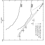
Figure 4: The CGB from SNI, SNII (including long-lived isotopes), in comparison to recent CGB measurements from HEAO-1 A4 (Kinzer et al. (1997)), COMPTEL (Kappadath et al. (1996)), and SMM (Watanabe et al. (1997)). For the SMM data the dashed-dotted lines indicate the $\pm$ 1$\sigma$ region of uncertainty of the averaged spectrum. Predictions for the background contributions from Seyfert galaxies (Zdziarski et al. (1993)) are also shown (dashed line).

In Figure 4 we plot the theoretical estimates together with existing measurements of the CGB. The standard model is apparently able to explain the bulk of the $\sim$ 1 MeV observed flux. In fact, for certain choices of model parameters $\gamma$-ray overproduction occurs, so that we are in principle able to constrain cosmological parameters and the cosmic star formation history. From the comparison of the different contributions it is clear that the MeV background is dominated by $\gamma$-rays from SNI. However, not all questions are answered. Even if the CGB is due to SNI, we must explain the apparent absence of a sharp drop in the observed flux above 3.5 MeV, where supernovae do not emit at all. Is it reasonable to expect blazars to fill in the gap in just the right way to explain the nearly continuous power-law behavior of the CGB? Too little is known about blazar spectra in this energy range (Bloemen et al. (1995); Blom et al. (1995)). The smooth continuation of the SMM data from 2 MeV to 6 MeV might indicate that SNI contribution to the flux near 1 MeV is only a small fraction. A similar problem is apparent at lower energy (few 100 keV), where Seyfert spectra fall rapidly and supernovae create only a flat spectrum.

Let us place this result (Figure 4) in perspective: the most plausible origin of the CGB in the soft $\gamma$-ray region ($<0.5$ MeV) appears to be a sum of unresolved Seyfert galaxies (e.g. Zdziarski et al. (1993); Zdziarski (1996)), which is consistent with balloon observations (e.g. Kinzer et al. (1978)). In the hard $\gamma$-ray region ($>10$ MeV), unresolved blazars are successfully invoked (e.g. Stecker & Salamon (1996)) to match high-energy EGRET observations (Cheng and Mukerjee (1998); Sreekumar et al. (1998)). The spectral properties of Seyfert galaxies and blazars leave a window around 1 MeV in which their integrated fluxes would be far below the observed level (Kappadath et al. (1996); Watanabe et al. (1997)). It is perhaps reassuring that our standard model for the supernova contribution is within a factor two of the observations, which argues for SNI as the primary explanation of the bulk, or all, of the MeV background. This fact is exploited below to generate constraints on the cosmic star formation history. However, we note the discrepancy between the combined Seyfert/Ia prediction and the data around 400 keV, perhaps hinting at a so far undetected population of sources or else suggesting that a fraction of Seyferts may have harder spectra than those found so far with the Compton Observatory.

As apparent in Figure 4 the line features at 847, 1238, 1770, 2030 and 2599 keV due to $\gamma$-ray line emission from the decay chain ${}^{56}{\rm Ni}\rightarrow$ ${}^{56}{\rm Co}\rightarrow$ ${}^{56}{\rm Fe}$ are not washed out completely, but still imprint a step structure in the CGB spectrum. So far one (unsuccessful) attempt was made to detect these edges (Barthelmy et al. (1996)), leaving a significant challenge for other current and also for future observations in the MeV regime.

5.1 Progenitors of Type Ia Supernovae

A satisfactory progenitor scenario for SNI has not yet emerged (e.g., Nomoto et al. (1997); Trimble & McFadden (1998)). Leading models invoke single-degenerate (SD) (Whelan & Iben (1973); Iben & Tutukov (1984)) or double-degenerate (DD) systems (Webbink (1984); Iben & Tutukov (1984)),i.e., distinguished by the nature of the white dwarf companion. Models of the explosion are sensitive the mass of the white dwarf. One refers to Ch or sub-Ch models, depending on the mass of the unstable white dwarf relative to the Chandrasekhar limit. We might learn something about the right progenitor systems through observations of the delay between star formation and Ia occurrence, which one might be able to derive from the observation of the relative I/II supernova rate as a function of redshift (Madau (1998); Sadat et al. (1998); Ruiz-Lapuente & Canal (1998)). Timescales of SNI explosion in both model classes depend on various parameters, such as the initial separation and the mass ratio of two WDs in DD models and length of time spent filling the Roche lobe in SD models (Madau (1998)). This time delay of SNI explosion after the global SFR can be $\sim 10^{9}$ yrs or as short as $\sim 10^{7}$ yrs (e.g., Ruiz-Lapuente & Canal (1998)), depending on the particular scenario under consideration. Following Madau (1998) we employed a characteristic explosion (delay) time scale ($\tau_{I}$), defining the explosion probability per white dwarf, and assume $\tau_{I}$ to be epoch independent. Given the vast uncertainties in the Ia heritage, we consider three cases:$\tau_{I}$ = 0.0, 1.5, and 3.0 Gy. Figure 5 shows the effects of these choices. Note that we keep the ratio of I/II = 1/3 at z=0 for any cases.

5.2 Constraints on the Cosmic Star Formation History

Figure 6 shows the evolution of the supernova rate as a function of look-back time (which depends somewhat on our choice of cosmological parameters). Figure 7 shows the same functions, but displayed in redshift space. The normalization is $R_{II}$(z=0) = 1. As discussed above, the function for SNII is identical to (our fit of) the observed star formation rate history, while the SNI curve shows a delay, but is normalized to give a present-day ratio of SNI/SNII = 1/3. This ratio decreases with redshift (Figure 8), resembling the trend predicted by population synthesis models (e.g., see Figure 5 in Yungelson & Livio (1998)).

Figure 9 shows multiple curves indicating how the CGB grows with maximum redshift included. Here redshifts up to 0.5, 1.0, 1.5, 2.0 and 5.0 are plotted, showing that most of the CGB comes from SFR at redshift less than $\sim$ 1.5, so that our results are insensitive to the possibly large uncertainties in measurements of the cosmic star formation rate at high redshifts. We also considered star formation histories in which the rate remains constant between z = z_p and z = 5, but this affects only emission from high redshift so that the correspondingly shifted supernova spectra contribute in an energy regime that is completely dominated by other sources. In other words, measurements of the MeV background are not able to constrain the SFR at high redshift. The situation is far better for the recent SFR history, which is the last point of discussion.

For a given delay time $\tau$ the supernova-induced CGB is mostly determined by the location and strength of the peak in the cosmic star formation history. In general, a shorter delay and/or smaller $z_{p}$ will increase the CGB. If the delay is zero, the CGB is inversely proportional to the location of $z_{p}$ (in our simple representation of the SFR with two power laws). Placing the time of the peak of star formation rate at larger redshift reduces the CGB. Of course, the total integrated flux also depends on the assumed I/II ratio, and the overall amplitude of the SFR. The current observational status of the SFR history (e.g. Lilly et al. (1996); Connolly et al. (1997); Sadat et al. (1998); Madau (1998); Guzman et al. (1998)) suggests values around (z_p, $\eta(z_{p})$ = (1$-$2,10$-$30). These values do not lead to a conflict with the measured CGB. Any increase in nickel yields in an average SNI or a global increase in the I/II ratio would eventually conflict with the CGB observations, which therefore provides an independent constraint on the global properties and cosmic evolution of Type Ia supernovae. While the constraints on cosmological parameters (H₀ and $\Omega$) do not lead to improvements over other methods, the CGB provides a unique handle on the unknown delay parameter $\tau_{I}$.

While the increase of the SFR with redshift by a factor 20$\pm$10 to the peak location z_p remains a robust conclusion of recent studies of the SFR, the normalization has been challenged. A new determination of the local volume-averaged star formation rate from the 1.4 Ghz luminosity function of star forming galaxies (Serjeant et al. (1998)) implies a local SFR density 2$-$3x larger than the Gallego et al. H_α estimate. Tresse and Maddox (1998) have shown the H_α luminosity function at z = 0.2, and their data suggest a SFR twice that determined from UV measurements. A similar shortfall of UV-based estimates in comparison to those derived from Balmer lines was reported by Hlazebrook et al. (1998) who used J-band IR spectroscopy of a redshift selected sample of 13 galaxies from the Canada-French Redshift Survey (CFRS) to measure the H_α luminosity function at z = 1. These observations also indicate elevated SFR values (factor 2$-$3) relative to values derived from the UV. We already mentioned the deep submillimeter survey of the HDF (Hughes et al. (1998)), which implies a star formation rate for z = 2$-$4 that is five times higher than that derived from optical and UV observations of the HDF. The interpretation of these differences involves the well known fact that star formation occurs in dense molecular regions which hides the optical and UV emission due to substantial extinction. That much of the cosmic star formation activity occurs in very dusty regions is also supported by observations of the IR background in the 140$-$240 $\mu$m region, which was recently detected by the DIRBE and FIRAS experiments aboard COBE (Dwek et al. (1998) and references therein). The IR background data also show that the UV and optically determined star formation rates fall short in producing the IR background, and specifically require the peak star formation rate (at z $\sim$ 1.5) to be larger by at least a factor two (Dwek et al. (1998)). These various recent claims strongly suggest that the SFR(z) function we use as “standard model” should be multiplied by a factor 2$-$3 at all redshifts! This would simply mean that we have to multiply the CGB fluxes by the same factor. Without the delay of SNI explosions this would yield a CGB spectrum in excess of the observed values, while for a 3 Gyr delay the model matches the observed flux. With the revised SFR values we can thus explain all of the CGB with emissions from Type Ia supernovae, and one does not need to invoke a new source population. However, a delay of 3 Gy is on the extreme side of the suggested values. It is clear that the CGB significantly constrains the properties of SNI and possible further increases in SFR values. If future observations can provide an accurate functional form for SFR(z), the CGB can be used to constrain supernova models. However, if SFR(z) estimates continue to be revised, the CGB provides a useful upper limit.

6 Conclusions

We calculated the contribution of supernovae to the cosmic $\gamma$-ray background (CGB). Following The et al. (1993) we used models W7fm and W10HMM as source templates for SNI and SNII, respectively. Our approach differs from that of The et al. (1993) through the use of the observed star formation history of the universe, obtained from Ly$\alpha$ QSO absorption studies (e.g., Pei & Fall (1995)), galaxy redshift surveys (e.g., Lilly et al. (1996)), broad band photometry of galaxies in the Hubble Deep Field (e.g., Madau et al. (1996)),and other recent work in this very active area of observational cosmology. We consider time delays of 0$-$3 Gy between SNII and SNI explosions. Our estimated background spectra are similar to those derived by The et al. (1993). We confirm their finding that SNII contribute very little ($\sim$ 1 %) to the CGB. SNI on the other hand, could explain most or all of the observed CGB spectra, for certain parameter choices. However, the standard model does not match the observed flux of the CGB, which suggests that either the current flux measurements are still an overestimate, that there could still be an unrecognized source population making a substantial contribution to the MeV background, or that the cosmic star formation rate is significantly higher than commonly assumed. This discrepancy would become even more serious if the SNI delays were much larger than 1 Gy, and/or if most of the cosmic star formation activity occurred at redshifts past z = 1. For example, combining Madau’s rates and a 2 Gy delay leads to a CGB flux that falls short of the observations by more than a factor three. On the other hand, short delays (less than 1 Gy) combined with a star formation history that has an increase of 10-30 by z_p = 1 yield a CGB flux that is just sufficient to explain the observations in a limited range of photon energies. We conclude from this, that the currently favored scenarios of SNI progenitors and their cosmic rate evolution underpredict the CGB. Recent upward revisions of the cosmic star formation history at all redshifts increase the predicted CGB fluxes, compensating the shortfall. However, an increase by a factor 2$-$3 overproduces the CGB unless the SNI delay time scale is much larger than 1 Gyr.

While it can not be proven, it also can not be ruled out that SNI could provide most or all of the CGB. If that were the case, theory predicts strong spectral steps in CGB due to line features from the ${}^{56}{\rm Ni}\rightarrow$ ${}^{56}{\rm Co}\rightarrow$ ${}^{56}{\rm Fe}$ decay. These have not yet been observed, but remain a challenge to current and future $\gamma$-ray experiments. Some fraction of the CGB (mostly below each of the major line energies) must be non-isotropic, because the high energy end of each line is due to emission from the nearest galaxies, which are known to have a very non-uniform spatial distribution to distance of $\sim$ few 100 Mpc (or redshift of z $\sim$ 0.1). The angle averaged spectrum out to z = 0.1 integrated over energy (thus the number of photons $cm^{-2}s^{-1}ster^{-1}$) is about 2% of the total (integrated to z = 5). Thus, to see the anisotropy in this energy range one would need new detectors that can detect the CGB to 1% accuracy.

The $\gamma$-ray background in the MeV regime provides valuable constraints on global iron synthesis in the universe, the global rate of star formation, and yields and lifetimes of SNI progenitors. These constraints are complimentary to other astronomical methods. Current observations of the CGB in the MeV range can largely be explained as the unresolved superposition of $\gamma$-rays emitted by Type Ia supernovae. At present there is no unsurmountable conflict between the estimated SFR, I/II supernova rate ratio, nickel yields, Ia explosion time scales, and the observed CGB flux. However, the parameter ranges are significantly constrained and there are open questions about the quality of the CGB fit from the combination of Seyfert galaxies, SNe, and blazars.

Figure 1: The time integrated $\gamma$-ray continuum flux per ⁵⁶Ni nucleus for the SNII template model W10HMM (dashed line), and for the SNI template model W7fm (solid line). SNI dominate in the MeV regime, because of their larger fraction of escaping $\gamma$-rays. SNII dominate at lower energies, but in this regime the CGB is overwhelmingly determined by X-ray emission from Seyfert galaxies.

Figure 2: The CGB contribution from SNI based on the SFR evolution function $\eta$ (eq. 12) with A = 4, B = 0.25, $z_{p}$ = 1, and 1.5 Gy time delay for SNI. Three values for the Hubble constant are presented. For comparison we also show the results of The et al. (1993), multiplied by 2/3 (based on the assumption that 2/3 of the cosmic iron production can be attributed to Type Ia supernovae; Thielemann et al. (1991)).

Figure 3: Type II supernovae contributions to the CGB from ${}^{56}{\rm Ni}\rightarrow$ ${}^{56}{\rm Co}\rightarrow$ ${}^{56}{\rm Fe}$ decay $\gamma$-lines and their corresponding comptonized $\gamma$-ray photons including long-lived line afterglows due to ²⁶Al, ⁴⁴Ti, ⁶⁰Co, and positrons.

Figure 5: Effects of the characteristic explosion/delay time scale ($\tau_{I}$, see text) of SNI relative to SNII which directly trace the cosmic star formation history. Three cases are shown:$\tau_{I}$ = 0.0, 1.5, and 3.0 Gy. Note that we keep the SNI/SNII ratio at z = 0 fixed at 1/3 in all cases. The comparison to the preliminary SMM estimates of the CGB (Watanabe et al. (1997)) shows that large delays lead to a CGB flux that significantly falls short of the observed spectrum.

Figure 6: Normalized SN rates in function of look-back time. The SNII rate (dashed line) is normalized at today. The SNI rate (solid line) has a delay time from a birth of a WD to the SN explosion. For simplicity we adopted a mean lifetime of SNI progenitors of 1.5 Gy which was obtained from the chemical evolution study (Yoshii et al. (1996)). Note that different $\xi_{SN}$ in Eq. (6) are used for each type of SN.

Figure 7: Same as Figure 6, but as a function of redshift (z). Transformation between z and t involves a model dependent look-back time.

Figure 8: The ratio of the SNI rate to the SNII rate as a function of redshift. The ratio is nearly constant for $z>1$ but rapidly increases towards small z, reaching 1/3 at z = 0 according to our adopted normalization for the present-day derived from local supernovae surveys (see text).

Figure 9: Curves indicating how the CGB grows with integration to maximum redshifts 0.5, 1.0, 1.5, 2.0 and 5.0 (no SNI delay was assumed for this calculation). The figure illustrates that most of the CGB is due to emission from redshifts smaller than the peak resdhift of the cosmic star formation history.

References

- Arnett (1996) Arnett, D., Supernovae and Nucleosynthesis, Princeton University Press, Princeton, NJ, 1996
- Barthelmy et al. (1996) Barthelmy, S. D., Naya, J. E., Gehrels, N., Parsons, A., Teegarden, B., Tueller, J., Bartlett, L. M. and Leventhal, M. 1996, Bull. American Astron. Soc., 189, #101.09
- Bloemen et al. (1995) Bloemen, H., Bennett, K., Blom, J. J., Collmar, W., Hermsen, W., Lichti, G. G., Morris, D., Schoenfelder, V., Stacy, J. G., Strong, A. W., Winkler, C. 1995, A&A, 298, L1
- Blom et al. (1995) Blom, J. J., Bennett, K., Bloemen, H., Collmar, W., Diehl, R., Hermsen, W., Iyudin, A. F., Schönfelder, V., Stacy, J. G., Steinle, H., Williams, O. R. and Winkler, C. 1995, A&A, 298, L33
- Bodansky, Clayton, Fowler (1968) Bodansky, D., Clayton, D. D., Fowler, W. A. 1968, Phys. Rev. Letters, 20, 161
- Cappellaro et al. (1997) Cappellaro, E., et al. 1997, AA 322, 431
- Cheng and Mukerjee (1998) Cheng, J., Mukherjee, R. 1998, ApJ496, 752
- Clayton & Silk (1969) Clayton, D. D. and Silk, J. 1969, ApJ,158,L43
- Clayton & Ward (1975) Clayton, D. D. and Ward, R. A. 1975, ApJ,198,241
- Cole et al. (1994) Cole, S., Aragon-Salamanca, A., Frenk, C. S., Navarro, J. F. and Zepf, S. E. 1994, MNRAS ,271,781
- Connolly et al. (1997) Connolly, A. J., Szalay, A. S., Dckinson, M., SubbaRao, M. U. Brunner, R. J. 1997,ApJ,486,L11
- Cowie et al. (1997) Cowie, L. X., Hu, E. M., Songaila, A., Egami, E. 1997, ApJ481, L9
- Dwek et al. (1998) Dwek, E., et al. 1998, ApJ, in press (astro-ph 9806129)
- Ellis et al. (1996) Ellis, R. S. et al. 1996, MNRAS 280, 235
- Gawiser & Silk (1998) Gawiser, E., Silk, J. 1998, Science, 280, 1405
- Gallego et al. (1995) Gallego, J., Zamorano, J., Aragon-Salamanca, A., Rego, M. 1995, ApJ,455, L1
- Hlazebrook et al. (1998) Glazebrook, K., Blake, C., Economou, F., Lilly, S., Colless, M. 1998, MNRAS, submitted (astro-ph 9808276)
- Guzman et al. (1998) Guzman, R., et al. 1998, ApJ489, 559
- Hughes et al. (1998) Hughes, D., Serjeant, S., Dunlop J., Rowan-Robinson, M., Blain, A., Mann, R. G., Ivison, R., Peacock J., Efstathiou, A., Gear, W., Oliver, S., Lawrence, A., Longair, M., Goldschmidt, P., Jenness, J. 1998, Nature, 394, 241
- Iben & Tutukov (1984) Iben, I. J. and Tutukov, A. V. 1984, ApJS,54,335
- Kappadath et al. (1996) Kappadath, S. C., Ryan, J., Bennett, K., Bloemen, H., Forrest, D., Hermsen, W., Kippen, R. M., Mcconnell, M., Schönfelder, V., Van Dijk, R., Varendorff, M., Weidenspointner,G. and Winkler, C. 1996, A&AS, 120,619
- Kinzer et al. (1978) Kinzer, R. L., Johnson, N. W. and Kurfess, J. D. 1978, ApJ, 222,370
- Kinzer et al. (1997) Kinzer, R. L., Jung, G. V., Gruber, D. E., Matteson, J. L. and Peterson, L. E. 1997, ApJ, 475,361
- Lilly et al. (1996) Lilly, S. J., Le Fevre, O., Hammer, F. and Crampton, D. 1996, ApJ,460,L1
- Madau et al. (1996) Madau, P., Ferguson, H. C., Giavalisco, M. E., Steidel, M., Fruchter, A. 1996, MNRAS 283, 1388
- Madau (1998) Madau, P. 1998, preprint astro-ph/9801005
- Mazalli et al. (1997) Mazzali, P. A., et al. 1997, MNRAS 284, 151
- Nomoto et al. (1984) Nomoto, K., Thielemann, F. -K. and Yokoi, K. 1984, ApJ,286,644
- Nomoto et al. (1997) Nomoto, K., Iwamoto, K., Kishimoto, N. 1997, Science, 276, 1378
- Pain et al. (1997) Pain, R., et al. 1997, ApJ473, 356
- Pagel (1995) Pagel, B. E. J. 1995, Rev. Mex AA 3, 125
- Peebles (1993) Peebles, P.J.E.,Principles of Physical Cosmology, Princeton University Press, Ewing, NJ, 1993
- Pei & Fall (1995) Pei, Y. C. and Fall, S.M. 1995, ApJ,454,69
- Perlmutter et al. (1997) Perlmutter, S., et al. 1997, IAU Circ. 6596
- (35) Pinto, P. A. and Woosley, S. E. 1988a, Nature ,333,534
- (36) Pinto, P. A. and Woosley, S. E. 1988b, ApJ, 329,820
- Prantzos (1993) Prantzos, N. 1993, A&AS, 97, 119
- Purcell et al. (1997) Purcell, W. R., Cheng, L. -X., Dixon, D. D., Kinzer, R. L., Kurfess, J. D., Leventhal, M., Saunders, M. A., Skibo, J. G., Smith, D. M. and Tueller, J. 1997, ApJ,491,725
- Ruiz-Lapuente & Canal (1998) Ruiz-Lapuente, P. and Canal, R. 1998, ApJ,497,L57
- Sadat et al. (1998) Sadat, R., Blanchard, B. and Silk, J. 1998, A&A ,331,L69
- Serjeant et al. (1998) Serjeant, S., Gruppioni, C., Oliver, S. 1998, MNRAS, submitted (astro-ph 9808259)
- Sreekumar et al. (1998) Sreekumar, P., Bertsch, D. L., Dingus, B. L., Esposito, J. A., Fichtel, C. E., Hartman, R. C., Hunter, S. D., Kanbach, G., Kniffen, D. A., Lin, Y. C., Mayer-Hasselwander, H. A., Michelson, P. F., Von Montigny, C., Muecke, A., Mukherjee, R., Nolan, P. L., Pohl, M., Reimer, O., Schneid, E., Stacy, J. G., Stecker, F. W., Thompson, D. J. and Willis, T. D. 1998, ApJ, 494, 523
- Stecker & Salamon (1996) Stecker, F. W. and Salamon. 1996, ApJ,464,600
- The et al. (1990) The, L.-S., Burrows, A. and Bussard, R. 1990, ApJ,352,731
- The et al. (1993) The, L.-S., Leising, M. D. and Clayton, D. D. 1993, ApJ,403,32
- Thielemann et al. (1991) Thielemann, F.-K. et al. 1991, Supernovae, ed. S Woosley (New York: Springer-Verlag),609
- Timmes et al. (1995) Timmes, F. X., Woosley, S. E., Hartmann, D. H., Hoffman, R. D., Weaver, T. A. and Matteucci, F. 1995, ApJ,449,204
- Timmes et al. (1996) Timmes, F. X., Woosley, S. E., Hartmann, D. H. and Hoffman, R. D. 1996, ApJ,464,332
- Timmes et al. (1997) Timmes, F. X., Diehl, R. and Hartmann, D. H. 1997,ApJ, 479,760
- Tinsley & Danly (1980) Tinsley, B. M., Danly, L. 1980, ApJ 242, 435
- Tonry et al. (1997) Tonry, J., et al. 1997, IAU Circ. 6646
- Tresse & Maddox (1998) Tresse, L., Maddox, S. J. 1998, ApJ495, 691
- Treyer et al. (1997) Treyer, M. A., et al. 1997, in “The UV Universe at low and high redshifts”, eds. W. Waller, et al. 1997, AIP (N.Y.), in print
- Trimble & McFadden (1998) Trimble, V., McFadden, L.-A. 1998, PASP 110, in press
- Tsujimoto et al. (1995) Tsujimoto, T., Nomoto, K., Yoshii, Y., Hashimoto, M., Yanagida, S. and Thielemann, F. -K. 1995, MNRAS, 277,945
- Turrato et al. (1996) Turrato, M., et al. 1996, MNRAS 283, 1
- Vacca & Leibundgut (1996) Vacca, W. D., Leibundgut, B. 1996, ApJ471, L47
- Watanabe et al. (1997) Watanabe, K, Hartmann, D.H., Leising, M.D., Share, G.H. and Kinzer, R.L. 1997, in the Proceedings of the Fourth CGRO Symposium, AIP 410, eds. C. D. Dermer, M. S. Strickman, and J. D. Kurfess, pp. 1223
- Webbink (1984) Webbink, R. F. 1984, ApJ, 227, 355
- Weinberg (1972) Weinberg, S., Gravitation and Cosmology, John Wiley and Sons, NY, 1972
- Whelan & Iben (1973) Whelan, J., and Iben, I. J. 1973, ApJ, 186,1007
- Williams et al. (1996) Williams, R. E., et al. 1996, ApJ, 479, L121
- Yoshii et al. (1996) Yoshii, Y., Tsujimoto, T. and Nomoto, K. 1996,ApJ, 462,266
- Yungelson & Livio (1998) Yungelson, Y., and Livio, M. 1998,ApJ, 497,168
- Zdziarski et al. (1993) Zdziarski, A. A., Zycki, P. T. and Krolik, J. H., 1993, ApJ, 414, L81
- Zdziarski (1996) Zdziarski, A. A. 1996, MNRAS, 281, L9