Hydrodynamical simulations of galaxy properties: Environmental effects

Abstract

Using $N$-body+ hydro simulations we study relations between the local environments of galaxies on $\approx 0.5{\rm Mpc}$ scale and properties of the luminous components of galaxies. Our numerical simulations include effects of star formation and supernova feedback in different cosmological scenarios: the standard COBE-normalized Cold Dark Matter model (CDM), its variant, the Broken Scale Invariance model (BSI), and a model with cosmological constant ($\Lambda$CDM). The present time corresponds to quite different stages of clustering in these three models, and the range of environments reflects these differences. In this paper, we concentrate on the effects of environment on colors and morphologies of galaxies, on the star formation rate and on the relation between the total luminosity of a galaxy and its circular velocity. We demonstrate a statistically significant theoretical relationship between morphology and environment. In particular, there is a strong tendency for high-mass galaxies and for elliptical galaxies to form in denser environments, in agreement with observations. We find that in models with denser environments (CDM scenario) $\sim 13$ % of the galactic halos can be identified as field ellipticals, according to their colors. In simulations with less clustering (BSI and $\Lambda$CDM), the fraction of ellipticals is considerably lower ($\sim 2-3$%). The strong sensitivity of morphological type to environment is rather remarkable because our results are applicable to “field” galaxies and small groups. Because of small box size (5 Mpc) we did not have large groups or clusters in our simulations.

If all galaxies in our simulations are included, we find a statistically significant dependence of the galaxy luminosity - circular velocity relation on dark matter overdensity within spheres of radius $0.5$Mpc, for the CDM simulations. But if we remove “elliptical” galaxies from our analysis to mimic the Tully-Fisher relation for spirals, then no dependence is found in any model.

1 Introduction

Most of our knowledge of the properties of galaxies derives from the light emitted by them, which in turn reflects the information contained in the baryonic component. In order to explain the origin of these properties, it is necessary to model the dynamics of the baryonic gas coupled gravitationally to the dark matter component. Previously, galaxy properties were studied using N-body simulations for the dark matter, and assuming different hypothesis to “extract” information for the baryonic component, e.g. linear biasing [Kaiser 1984] or constant M/L. Improvements in computational techniques and resources have made it possible to include gas dynamics in N-body simulations [Evrard 1988, Cen et al. 1990, Katz and Gunn 1991].

In addition to purely gravitational and hydrodynamical effects, it is essential to include complex local processes that affect the energy budget of the gas, such as radiative cooling or photoionization heating by an UV background. It is also important to consider effects of stellar formation and evolution and feedback processes produced by the explosions of supernovae. Self consistent modeling of all these physical processes in cosmological simulations is crucial for attaining insight into the generation and evolution of galaxies within a given cosmological scenario.. However, numerical simulations invariably include various approximations and simplifying assumptions regarding the relevant physical processes; these assumptions need to be verified. In recent years there has been a tremendous accumulation of observational data shedding light on the underlying properties of galaxies. The observations also allow us to constrain the assumptions in numerical modeling of the complex baryonic processes involved in galaxy formation and evolution.

As an alternative to the use of direct numerical simulations of the most important relevant physical phenomena, much of the effort toward modeling relationships between environment and observational properties of galaxies up to now has been focussed on ”semi-analytical” approaches to galaxy formation and evolution [White and Frenk 1991, Kauffmann et al. 1993, Lacey and Cole 1993, Cole et al. 1994, Heyl et al. 1995, Baugh et al 1997]. However, although quite a bit has been learned from semi-analytical models, there are certain processes that they are simply not designed to incorporate. In particular, the ability to take nonlinear hydrodynamical processes and their interactions with other physical processes properly into account is limited. Hydrodynamical effects could in principle be implemented in a semi-analytical approach, but this would require some kind of prior knowledge to identify the most important consequences and insert their effects correctly by hand. It is not clear whether the effort required to do so is less than that required to simulate the whole problem including hydrodynamics self-consistently right from the start.

In this article, we study environmental effects on observable galaxy properties such as colors, morphology, star formation rates, and magnitude-circular velocity relations by means of numerical simulations. For these simulations, we have adapted and applied the N-body (PM) + Eulerian hydro code (Piecewise Parabolic Method [Colella and Woodward 1984]) reported in Yepes, et al. [1997], (YK³). As described below, this code is designed to model those processes generally thought to be most relevant at the scales we are considering. The universe is modeled as a 4-component medium consisting of dark matter, stars, “hot” or ambient gas, and cold clouds. Star formation depends on the local density of cold gas clouds and is regulated by the supernova feedback loop. In particular, star formation is modeled by converting cold gas clouds at a certain rate into discretized particles, each of which may be idealized as representing a “starburst.” Stellar population synthesis models [Bruzual and Charlot 1993] are then used to derive the luminosities and colors of the resulting galaxies.

To add more breadth to our analysis of environmental effects, it is useful to consider the evolution of this 4-component medium in the context of several rather different cosmological scenarios:

1. Standard unbiased Cold Dark Matter model (CDM).

2. Model with a cosmological constant ($\Lambda$CDM).

3. Broken Scale Invariance (BSI) [Kates et al 1995].

These distinct scenarios allow us to compare how different growth rates in cosmological models (e.g., CDM vis. $\Lambda$CDM) and different epochs of structure formation (CDM vis. BSI) affect the final properties of galaxies. However, since it is difficult to control for confounding factors such as the influence of the box size, this paper is not intended to distinguish a preferred cosmological model.

The paper is organized as follows. Section 2 briefly reviews the hydrodynamical model used, describes the halo identification algorithm and the technique for assigning luminosities to these halos and discusses the characteristics of the numerical experiments. Section 3 describes the general properties of the distribution of the four components of matter in the simulations. Section 4 summarizes the quantitative analysis of the effects of environment on galaxy properties. The conclusions are given in Section 5.

2 Simulations

2.1 Description of the hydrodynamical model

The code which we have applied to this problem has been designed and tested (YK³) to provide a phenomenological description of the interaction between the gas and the stellar component, simulating the physical processes most relevant for galaxy formation:

(i) 3D hydrodynamics (including a shock capturing technique), (ii) the dynamics of the interstellar medium, modeled as a two-phase medium (ii) radiative and Compton cooling of the gas, (iii) star formation and heating of the gas by supernovae explosions (”supernova feedback”).

Here, we summarize the equations governing the cooling of the gas, star formation, and the effects of supernovae in a slightly simplified form. The main characteristics of the code were discussed in detail in YK³.

The code models two mechanisms for transferring gas from the hot component with density $\rho_{h}$ to the cold component with density $\rho_{c}$: The latter (“cold clouds”) are intended to represent structures where star formation occurs, such as Giant Molecular Clouds in our galaxy. If the gas temperature in a cell $T_{h}$ drops below $T_{lim}=2\times 10^{4}$ K and the density of the gas exceeds a threshold, all the hot gas in the cell is transferred to the cold component, thus enabling star formation. The condition on the gas density is expressed in the form $\rho_{\rm gas}>{\mathcal{D}}\;\Omega_{B}\rho_{cr}$, where $\Omega_{B}\rho_{cr}$ is the mean density of the baryons in the Universe. The adjustable parameter ${\mathcal{D}}$ is introduced [Mücket and Kates 1997] in order to take into account heating of the gas by an ionizing ultraviolet background due to quasars and active galactic nuclei [Giroux and Shapiro 1986, Petitjean et al. 1995, Mücket et al. 1996]: at lower densities the gas is significantly heated by the UV flux and cannot form stars. Here, we took ${\mathcal{D}}=100$. This mechanism also prevents star formation outside of galaxies.

Another mechanism for formation of cold gas clouds is by means of the thermal instability [McKee and Ostriker 1977]. The temperature range for production of cold clouds via thermal instability is taken to be $T_{h}<T_{inst}$, where in this paper $T_{inst}\sim 5\times 10^{5}$ K. To compute the rate of mass increase in cold clouds, we suppose that all of the energy emitted by the hot gas is really lost by the gas which goes from hot to cold. If we suppose in addition that the gas is ideal and cannot cool below $T_{lim}$, then we obtain the expression

$$\left(\frac{d\rho_{h}}{dt}\right)=-\left(\frac{d\rho_{c}}{dt}\right)=-C\frac{\Lambda_{r}(\rho_{h},T_{h})}{\gamma\epsilon_{h}-\epsilon_{c}},$$ (1)

where $\gamma$ is the ration of specific heats of an ideal gas, $\epsilon$ is the thermal energy per unit mass of gas, $\Lambda_{r}$ is the cooling rate due to radiation, and the factor $C=1-10$ is introduced to characterize the uncertain effects of unresolved substructure. Nevertheless, at it was shown in $YK^{3}$, the results are not sensitive to the value of the $C$ parameter.

Because of the frequent exchange of mass between the hot and cold gas phases, it is reasonable to consider the hot gas and cold clouds as one fluid with rather complicated chemical reactions going on within it. The two components are assumed to be in local pressure equilibrium so that $P_{\rm gas}=P_{c}=P_{h}\equiv(\gamma-1)u_{h}$, $u_{h}=\rho_{h}\epsilon_{h}$, where $u$ is the internal energy per unit volume and $P_{\rm gas}$ is the internal gas pressure.

Star formation is assumed to occur only in cold clouds. Stars with masses exceeding $(10-20)M_{\odot}$ undergo supernova explosion within a single simulation timestep. If we suppose that the stars that explode on this short timescale constitute a fraction $\beta$ of the total, the rate of formation of long-lived stars becomes

$$\frac{d\rho_{*}}{dt}=\frac{(1-\beta)\rho_{c}}{t_{*}},$$ (2)

where $t_{*}=10^{8}$yr is the time scale for star formation. The value of $\beta$ is sensitive to the shape of the initial mas function (IMF), especially the lower limit. In our simulations we have taken $\beta=0.12$ corresponding to the Salpeter IMF. In view of the uncertainties in supernova energy, the energy input due to lower-mass stars, $(7-10)M_{\odot}$, is not included here. The evaporation of cold clouds in the interstellar medium due to supernova explosions is incorporated into the code by supposing that the total mass of cold gas transferred to the hot gas component is not just the mass in the star itself, but a factor of $A$ times the supernova mass. Each $1M_{\odot}$ of supernovae dumps $4.5\times 10^{49}$ ergs of heat into the interstellar medium and evaporates a mass $A\cdot M_{\odot}$ of cold gas. This “supernova feedback parameter” $A$ could well depend on local gas properties such as density and chemical composition. Previous results ($YK^{3}$) point to a large value of $A$. An especially sensitive test is provided by the Tully-Fisher relation [Elizondo et al. 1998]. Here, we will assume $A$ to be constant and large ($A=200$) resulting in low efficiency of converting cold gas into stars. The mass transfer between different components, due to evaporation, is defined by:

$$\left(\frac{d\rho_{h}}{dt}\right)_{evap}=-\left(\frac{d\rho_{c}}{dt}\right)_{evap}=\frac{A\beta\rho_{c}}{t_{*}}$$ (3)

Another important effects of supernovae explosions is the injection of metals to the surrounding gas, which modifies its cooling properties. In order to incorporate the effects of metallicity in our code, we assume solar abundance in regions where previous star formation has occurred. Otherwise, the region is not considered to be enriched with metals, and cooling rates for a gas of primordial composition are assumed.

Because supernova feedback regulates star formation efficiency in halos, the value of $A$ would be expected to play an important role in the observational consequences of our results. Hence, comparison with observations should provide useful information on supernova feedback. For this reason, several of the simulations reported in Table (1) have been rerun with different values of $A$, in order to study the effects of feedbacks on the observational properties of galactic halos. In previous work, we have paid particular attention to the effects of feedback on the characteristics of the magnitude-circular velocity (Tully-Fisher) relation and on the faint end of the luminosity functions in different photometric bands [Yepes and Elizondo 1997]. We have seen that supernova feedback is responsible mainly for the determination of the slope of the Tully-Fisher: low $A$ values (large reheating) makes the low circular velocity halos fainter while hardly affecting the halos with large circular velocity. The scatter of the relation is reduced when low $A$ values are assumed, as compared with large $A$ values. In the case of no feedback ($A=0$), we get slopes and scatter that are inconsistent with the observational Tully-Fisher. Also, when no feedback is assumed, we get a faint-end luminosity function which is too steep (too many faint galaxies) as compared with the most recent estimates for the $B$ and $K$ bands. More detailed information on this analysis can be found elsewhere [Elizondo et al. 1998]. Here, we will focus our study on a possible dependence of the Tully-Fisher relation (see § 4.4) on environment.

2.2 Galaxy finding algorithm

Galaxy catalogs at selected redshifts were constructed from the simulation data as described in YK³. Briefly, local maxima of the dark matter density field are first identified on the grid. We next compute the mass inside spheres of 2-cell radius ( 78 kpc) centered at the center of mass of the local particle distribution. If the mass inside such a sphere exceeds the mass within a sphere of overdensity 200, we mark the 2-cell sphere as a dm halo. Otherwise, we repeat the process for a sphere of 1-cell radius ( 39 kpc). If the test succeeds, the matter within the sphere is assigned to the halo. If the test again fails, the local maximum is not considered to be a halo. Some dm halos have zero luminosity. In what follows, we use the term “galaxy” to refer to a halo with nonzero luminosity.

2.3 Assignment of magnitudes and luminosities

In order to assign luminosities and colors to the halos in which stars have formed, we need to know the spectral energy distribution (SED) $S(\lambda,t)$ for each halo as a function of time. This is possible since for each galaxy we have a list of starbursts and, associated with each, its mass and time of formation. These two parameters are sufficient for calculating the SED assuming an appropriate model for stellar population synthesis. Among the numerous stellar population synthesis models that have been proposed (see YK³ for references and discussion) we have chosen the model of Bruzual & Charlot (1993), which describes the time evolution (between 0 and 20 Gyr) of SED’s for a burst of star formation under conditions of solar metallicity and a Salpeter initial mass function, in accordance with the assumptions of the YK³ code.

Using this stellar population synthesis model, we compute the SED of each galaxy according to

$$S(\lambda,t)=\sum_{\tau_{i}}\Phi(\tau_{i}){\mathcal{F}}(\lambda,t-\tau_{i}),$$ (4)

where $\Phi(\tau_{i})$ is the mass of stars in the halo produced at timestep $\tau_{i}$ , and ${\mathcal{F}}(\lambda,t)$ is the SED due to a starburst of 1 $M_{\odot}$ after an evolution time $t$.

To obtain the absolute luminosity $L_{f}(t)$ in any given band, we convolve $S(\lambda,t)$ with the appropriate filter response function $R_{f}(\lambda)$. Combining the $L_{f}(t)$, we then obtain the evolution of the color index of the numerical galaxy. (Of course, the observed color of a real galaxy would be influenced by additional factors such as the interaction of starlight with the surrounding plasma). We have calculated the luminosities and colors of the galaxies in the various filters comprising the Johnson UBVRIK system.

2.4 Parameters of the simulations

Regarding our simulations as numerical experiments, our goal was to obtain a sufficiently large sample of “numerical galaxies” to permit reliable, i.e., statistically significant comparisons with observational quantities. To this end, a set of 11 simulations were performed for each of the CDM, $\Lambda$CDM ($\Omega_{\Lambda}=0.65$), and BSI models. COBE normalization was taken and baryon fractions were compatible with nucleosynthesis constraints [Smith et al. 1993] ($\Omega_{B}=0.051$ for BSI and CDM, $\Omega_{B}=0.026$ for $\Lambda$CDM ).

Due to limitations on computational resources affecting both the number of particles and the number of cells, the selection of a simulation volume requires a compromise among various considerations. On the one hand, we need to resolve scales on the order of the size of a galaxy, implying high resolution, but on the other hand the larger the volume, the more the simulations will be representative of the range of environments possible in the cosmological scenarios. Based on general considerations and on our experience with the performance of the code, we have taken a size of 5 Mpc but with different Hubble constants given by $h=0.7$ for the $\Lambda$CDM model and $h=0.5$ for the CDM and BSI simulations. In what follows, all lengths and masses are expressed relative to the corresponding Hubble constant of particular model (i.e., the units are scaled to “real” megaparsecs, and there are no $h$ terms).

Due to the small box size of our simulations, needed to properly resolve galaxies, most of the large-scale power of the density fluctuations is absent. In order to characterize the effects of the missing longer-wave fluctuations on the structures that are formed inside our boxes, we compute the linear theory mass variance,

$$\sigma^{2}_{L}(R)=\int_{2\pi/L}^{kmax}e^{-k^{2}R^{2}}P(k)k^{2}dk$$ (5)

with a Gaussian filter of $R=0.5$ Mpc for boxes of $L=5$ Mpc and for boxes of $L=10$ Mpc. The resolution is the same in both cases (same $kmax$). Here, we use a CDM power spectrum (Fig 5), but the results will be similar for other models because the spectra are basically parallel in the range of wavenumbers we are interested in. The ratio of mass variances is $\sigma_{10}(R=0.5)/\sigma_{5}(R=0.5)=1.12$. This linear estimate suggests that on scales of 0.5 Mpc, which is the one we will use to study the effects of environment, the effects of the missing power will not be very important ($\sim 12$%).

The simulations reported were performed in two SGI Power Challenge supercomputers at the CEPBA (Centro Europeo de Parelismo de Barcelona). The main characteristics of the simulations are given in Table (1).

Table 1: Parameters of the simulations.

Parameters	CDM	$\Lambda$CDM	$\Lambda$CDM	BSI
$\Omega_{\Lambda}$	0	0.65	0.65	0
$\Omega_{B}$	0.051	0.026	0.026	0.051
$\Omega_{dm}$	0.949	0.324	0.324	0.949
$h$	0.5	0.7	0.7	0.5
Simulation Box at $z=0$, ($h^{-1}$Mpc)	2.5	3.5	3.5	2.5
Cell size at $z=0$, ($h^{-1}$kpc)	19	27	13.7	19
Number of cells	$128^{3}$	$128^{3}$	$256^{3}$	$128^{3}$
Number of realizations	11	11	1	11
Mass Resolution for dark matter ($h^{-1}M_{\odot}$)	$2\times 10^{6}$	$1.3\times 10^{6}$	$1.6\times 10^{5}$	$2\times 10^{6}$
Total Number of galaxies	447	442	50	649
Total number of bright galaxies ($M_{B}\leq-16$)	73	91	8	144

The 11 simulations carried out for each model correspond to a total simulated comoving volume of 1375 Mpc³. The total number of numerical galaxies generated is of the order of $\sim 450$ for each model. This quantity of data permits construction of a reasonably large sample (data base) suitable for carrying out statistical analyses sensitive to the effects we would like to study and comparing with the appropriate observations.

2.5 Effects of resolution

In any cosmological hydrodynamical simulation, limitations on resolution give rise to a smearing of internal structures, which constitutes a potential source of error. The simulations reported here are no exception, because with a spatial resolution of 10 kpc to 40 kpc, we clearly do not resolve the internal structure of a galaxy. Limits on spatial resolution also degrade the time resolution of star formation, which is also limited for other reasons. Time resolution, though not often discussed, is of comparable importance to spatial resolution, because moderate but recent bursts of star formation that are not properly resolved (e.g., attributed to earlier times) can have a large effect on colors (see Fig. 2).

Having said all this, we note that for the most part global parameters (such as the total luminosity or maximum of the rotational velocity) turn out to be rather insensitive to resolution. This “robustness” was confirmed by comparing results of simulations made with the same initial conditions, but run at different resolutions. Some tests concerning the effects of the resolution were presented in YK$3$ and in Elizondo et al (1998), but due to the importance of this issue, we discuss some of them here:

In order to test the effects of spatial numerical resolution on the properties of the halos, we have run one simulation for the $\Lambda$CDM model, with the same box size and parameters as for the 11 simulations of the $\Lambda$CDM model given in Table 1, but with $256^{3}$ particles and cells (i.e. 19.5 kpc comoving and $2.3\times 10^{5}M_{\odot}$ mass per particle). We then reran this simulation at lower resolution with $128^{3}$ particles and cells. The initial particle distribution was generated according to the Zeldovich approximation. The displacement field used for the $128^{3}$ grid was generated by aggregating the displacement field over the 8 nearest-neighbor cells with respect to the $256^{3}$ grid. The high-resolution simulation produces about $\sim 25$% more galaxies, but the excess comprises primarily faint galaxies. The individual massive halos remaining at the end of evolution in both simulations could be identified one-to-one, which made possible a detailed and reliable comparison of the effects of resolution in the final observational properties of the halo distribution.

Figure 1: Effects of resolution on the circular velocity profile of the 4 most massive galaxies found in one $\Lambda$CDM simulation run with two different resolutions: $128^{3}$ and $256^{3}$ (column 3 of Table 1). Solid line is the circular velocity for the high-resolution simulation. Dashed lines correspond to the halos found in the same simulation but with lower resolution. The vertical dotted line represents the limiting radius for these galaxies according to our galaxy finding algorithm.

In Figure (1) we plot the circular velocity profile (($GM(r)/r)^{1/2}$) for the 4 biggest halos found in the $\Lambda$CDM simulations mentioned above. As can be seen, estimates of the circular velocity at the limiting radius for these halos differ by less than 10%.

The “robustness” seen here can be understood if we consider the evolution of the gas falling on a galaxy containing hot gas. For a large enough galaxy (where the limit for “enough” does depend on resolution) the gas cannot be pushed back too far even if the galaxy has a high star formation rate (SFR). Because the gas density close to a galaxy is high, it appears that the cooling time is always rather short (on cosmological scales). As the result, the gas keeps falling back on to the galaxy, cools even faster, and gets converted into stars. Because in our model the whole process of star formation from the gas (which determines the SFR and thus the luminosity) is regulated mostly by the rate of gas infall and by feedback (neither of which depend strongly on resolution), the luminosity and colors of the galaxy are remarkably unbiased with respect to resolution changes. However, there are clear limitations to this weak dependence on resolution: Small galaxies (in our case $M_{total}<3\times 10^{10}M_{\odot}$) are indeed sensitive to the resolution, because in their case the depth of the potential well is not accurately modeled.

Figure 2: Variation of the color indices ($U-B$,  $B-V$ and $R-K$) of the galaxies found in one $\Lambda$CDM simulation run with two different resolutions: $128^{3}$ and $256^{3}$, as a function of the halo mass. Filled circles represent galaxies brighter than $M_{B}\leq-16$. Open circles represent faint galaxies ($M_{B}>-16$).

In order to estimate the effects of numerical resolution on the morphological assignment used in this paper (see section 4.2), we have computed the color indices ($U-B$, $B-V$ and $R-K$) of the halos for the $\Lambda$CDM simulation run with $256^{3}$ particles and cells and those from the same halos found in the simulation rerun with lower resolution ( $128^{3}$ particles and cells). Fig. (2) shows the variation of the color indices as a function of the mass of halos found in the lower-resolution simulation From this figure we can conclude that the color indices of massive halos (i.e. $M\geq 3\times 10^{10}M_{\odot}$) are not very sensitive to resolution. Some of them do have bluer colors (specially $U-B$) in the high-resolution simulation due to a recent burst of star formation in those halos which did not occur in the low-resolution simulation. For these halos, the morphological assignment according to colors would have been affected by resolution. This is the sort of effect that would have been expected and should be kept in mind when interpreting the results. Nevertheless, the main conclusions of our qualitative study of the dependence of morphology on environment appear not to be seriously affected.

3 General Properties of the Simulations

We begin our description of the simulation results in our CDM, $\Lambda$CDM and BSI scenarios with some qualitative aspects of the simulated gas and dark matter distributions.

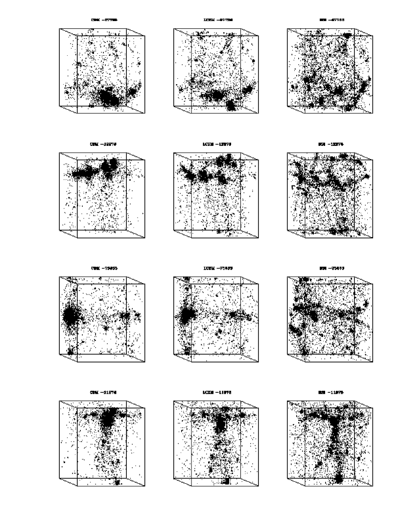
Figure 3: 3-dimensional distribution of 10% of the dark matter particle at $z=0$ for 4 of the 11 realizations. The first column represents CDM realizations, the second $\Lambda$CDM (LCDM) and the third is for the BSI. Each group of realizations (CDM, $\Lambda$CDM and BSI) was performed with the same random phases. The random seed chosen for the generation of the phases is indicated in each box. The box size is 5 Mpc

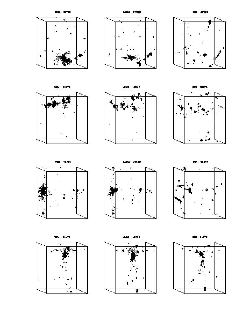
Figure 4: Same as in Fig. 3 but for the star particle distribution.

3.1 Dark matter distribution

Fig. (3) and (4) show the distribution of dark matter particles at redshift $z=0$ for each realization of the three scenarios considered. (Since only 10% of the particles have been plotted, some of the structures appear slightly washed out). One sees that both CDM and $\Lambda$CDM have given rise to numerous galaxies, with one predominant massive ($M\sim 10^{12}M_{\odot}$) galaxy generated by merger of different halos during the course of its evolution. In both cases, one observes a significant number of less massive halos distributed in a transitory (but still present) filament. In many simulations, the most massive galaxy is accompanied by neighboring halos with a mass of the order of $M\sim 5\times 10^{10}M_{\odot}$, which are destined to be absorbed by the main galaxy due to the intense gravitational attraction. A general trend in our results is that the massive halos in CDM are the product of a larger number of collapses than the ”corresponding” structures in in $\Lambda$CDM. This difference is especially evident in the four CDM realizations shown in Fig. 3) and (4), in which the massive galaxy is just merging with a neighbor or has just devoured one, whereas in the corresponding $\Lambda$CDM realizations the galaxies are still approaching. In the same manner, clustering is more pronounced in CDM than in the other scenarios. This result might at first seem puzzling in $\Lambda$CDM, since all other things being equal, the time available for evolution tends to be longer in models with a cosmological constant. However, our choice of parameters implies a similar evolutionary time for all the models under consideration, and hence the degree of clustering depends mainly on the initial power spectrum. As seen in Fig. (5), the CDM spectrum has a larger amplitude at the scales considered than $\Lambda$CDM; this difference is sufficient to explain the disparity between the two models.

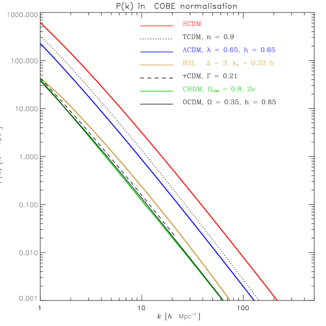
Figure 5: Power spectrum for eight of the most popular cosmological scenarios, at the scales relevant for our analysis. All of them are COBE normalized.

In the BSI models, the differences are even greater. The distribution of matter appears much more diffuse and the filaments more evident (see simulation 11978). The number of halos is much greater, but they are less strongly clustered than in the other two models (see 12278). The larger halos generated in BSI generally have lower masses than the corresponding ones in CDM and $\Lambda$CDM. It is evident that fewer mergers of halos have occurred and that the halos are distributed more evenly within the simulation volume. This property may also be attributed to the lower amplitude of the fluctuation spectrum. Nonetheless, there is a systematic relation in the evolution in CDM and BSI, since the spectra are essentially parallel in the dynamical range studied here. Hence, aside from an overall delay in the dynamical evolution of BSI models relative to the corresponding CDM realization, there is a great similarity in those dynamical properties and structures of the two models which depend mainly on the dark matter distribution (clustering, matter distribution, masses, etc.). Nonetheless, as will be seen in what follows, there are no correspondingly simple relations characterizing those properties which depend mainly on the baryonic component.

The above discussion concerning the similarity of BSI and CDM power spectra hardly applies to the $\Lambda$CDM model. The observable properties, especially with respect to the baryonic component in $\Lambda$CDM and CDM, are even more distinct due to the differences in the quantity of dark and baryonic matter, in expansion rates, and in the Hubble parameter.

3.2 Characteristic evolutionary stages of dark and stellar matter in the scenarios

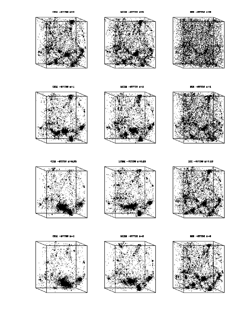
Figure 6: Redshift evolution, from $z=3$ to $z=0$, of the dark matter particle distribution for the realization 67736 in the three cosmological scenarios. 10% of dark particles are shown.

Numerical simulations offer a useful opportunity for studying how the distinct properties of halos evolve. Some qualitative insight into the evolution of the particle distribution is provided by Fig (6). The dark matter evolution from $z=3$ to $z=0$ is illustrated for the realization 67736 of all three scenarios (to be studied in more detail below). In these figures, one sees that CDM and $\Lambda$CDM follow a similar evolution up to about $z\sim 1$. Henceforth, a greater rate of collapse is observed in CDM.

Figure 7: Redshift evolution, of the RMS density fluctuations in a 5 Mpc box as predicted by linear theory, for the three cosmological scenarios.

A partial explanation is provided within the linear perturbation theory. In Fig 7 we plot the growth of the rms density fluctuations, as predicted by linear theory, in the 3 models. As can be seen, the growth rates for both $\Lambda$CDM and CDM are very similar up to $z\sim 1$, when the effects of the cosmological constant become relatively important (e.g. [Peebles 1980]). Before this epoch, there are some differences in the linear growth of fluctuations due to different power spectra and matter content. Nonetheless, similar structures are developed in both models up to $z\sim 1$. At later epochs, the growth rate of the density contrast in $\Lambda$CDM decreases almost to zero , which would explain the difference between its collapse time dependence and that of CDM.

The time scale for structure formation is also much longer in BSI. At $z=3$, small zones are generated in which matter accumulates leading to some star formation, although the overall distribution of dark matter is still rather uniform. It is not until about $z=1$ that a population resembling galaxies can be identified. Fig. (8) shows the number of numerical galaxies formed in all the BSI and CDM simulations at various redshifts (upper panel). In CDM, the number of galaxies formed has its maximum at $z=3$. Subsequently, the coalescence rate exceeds the formation rate, leading to a decrease of the total number. In contrast, the number of galaxies in BSI does not attain a maximum till $z\sim 0.25$, reaching a value similar to the maximum in CDM.

Figure 8: Redshift evolution of the total number of numerical galaxies found in all realizations of the BSI and CDM simulations (upper panel). Lower panel shows the evolution of the percentages of galactic type halos for three different mass ranges, in the BSI (dashed line) and CDM (solid line) simulations.

The galaxy mass function is shown in the lower panel. In CDM, the percentage of halos with mass in the range $10^{10}M_{\odot}<M\leq 10^{11}M_{\odot}$ is about 23% for $z=4$; already at this redshift there are quite massive galaxies present (3% of the galaxies with masses exceeding $10^{11}M_{\odot}$). In contrast, the BSI model in this box only yields 4% of galaxies with a mass in the range $10^{10}M_{\odot}<M\leq 10^{11}M_{\odot}$, and not a single one more massive than $10^{11}M_{\odot}$ at $z=4$. This relative delay in generating objects poses serious difficulties for this model, considering the presence of objects detected at $z\sim 4$ in some observations [Petitjean et al. 1996].

Returning to the similarity in structures generated in BSI at $z=0.25$ with those of CDM at $z=3$, we note that the relative delay in evolution is directly related to the difference in amplitude, $\delta\varepsilon=9$, between the power spectra $P^{CDM}(k)$ and $P^{BSI}(k)$ at the scales of interest (Fig. (5)); in linear theory, one may obtain an expression relating the epochs of similarly developed structures in the two models:

$$z^{CDM}=\sqrt{\delta\varepsilon}(z^{BSI}+1)-1.$$ (6)

Hence, the visual impression of similar structure at different redshifts can be explained by the relationship between the spectral amplitudes of the models.

3.3 Distribution of the baryonic component

Up to now, the information discussed is of the sort available from numerous N-body simulations. The inclusion of the various gas components in our simulations provides a basis for describing the properties of the baryons. Although the motion of the starburst particles is simulated by N-body techniques, their generation is directly related to the dynamics of the gas. Fig. (9) shows the densest region of simulation 67736 at $z=0$ in the three cosmological scenarios. It shows density isocontours of dark matter for $\rho_{dm}=30\rho_{cr}$ and of star density for $\rho_{*}=5\rho_{cr}$. Note that number of halos varies from model to model, being larger in BSI and smaller in $\Lambda$CDM. Many halos are not capable of generating enough stars; these dark halos are not seen in the dark matter particle distribution because of the low percentage of particles plotted. BSI exhibits a larger number of halos with stellar formation as well as a more homogeneous distribution and less merging, corresponding to a hierarchical structure scenario at a relatively early stage of evolution.

     

Figure 9: 3D Isodensity contours of dark matter (transparent grey) for $\rho_{dm}=30\;\rho_{cr}$ and of star density (yellow shading) for $\rho_{*}=5\;\rho_{cr}$ corresponding to the realization 67736 at $z=0$ in the three different scenarios: (a) CDM, (b) $\Lambda$CDM and (c) BSI. The region shown corresponds to the position of the most massive halo generated in the simulations. Full color figures are available in GIFF format at:http://astrosg.ft.uam.es/$\sim$gustavo/newast

It is interesting to note in Fig. (9) that the ability of the numerical model to generate a stellar component in the halo provides us with much more complete information about the internal structure of the halo. In this way, for the CDM scenario it is possible to identify two components of star formation in the interior of a halo, thus allowing one to describe the internal structure in much more detail than simply using dark matter. In particular, this type of analysis allows identification of several galaxies within one halo, which is important for drawing conclusions regarding the degree of collapse in a given galaxy formation model. This is an important advantage compared to N-body dark matter simulations, in which interacting halos mix and do not allow precise determination of the existence of several components in the same halo.

     

Figure 10: 3D isodensity contour of the gas distribution for $\rho_{\rm gas}=\rho_{cr}$ corresponding to the realization 67736 at $z=0$ in the three cosmological scenarios: (a) CDM, (b) $\Lambda$CDM and (c) BSI. The surface has been colored according to the gas temperature in this isodensity contour: red $T\sim 5\times 10^{5}$ K, yellow $T\sim 4-3\times 10^{5}$ K, green $T\sim 2.5\times 10^{5}$ K and blue $T\sim 5\times 10^{4}$ K. Full color figures are available in GIFF format at:http://astrosg.ft.uam.es/$\sim$gustavo/newast

A description of the gas distribution and temperature provides information on the dynamical evolution of the gas, as well as on the locations and the conditions under which stars are generated. Fig. (10) illustrates the $\rho_{\rm gas}=\rho_{cr}$ density isocontour. To gain more insight into gas dynamics, this surface has been shaded according to the gas temperature in the isocontour. The temperature ranges from $T\sim 5\times 10^{5}$ K (red shading) , $T\sim 3-4\times 10^{5}$ K (yellow), $T\sim 2.5\times 10^{5}$ K (green) and $T\sim 5\times 10^{4}$ K (blue). An isocontour of lower gas density $\rho_{\rm gas}=0.5\rho_{cr}$ is also shown in Fig. (11) with the same color scheme. In addition, the regions of gas temperature $T=2\times 10^{5}$ K (cloudy structure shape) are shown. The two figures reveal a predominant filamentary structure for the low-density gas regions. These filaments become more evident at lower density contours.

     

Figure 11: Same as Fig. 10 but for $\rho_{\rm gas}=0.5\;\rho_{cr}$. The regions of gas temperature $T\sim 2\times 10^{5}$ K are also shown, (transparent light brown color surface). Full color figures are available in GIFF format at:http://astrosg.ft.uam.es/$\sim$gustavo/newast

The most evident difference among the three scenarios is the existence of more filaments in BSI, compared to a lower number in CDM and $\Lambda$CDM, where the filaments are depleted. A general characteristic of the gas distribution is that the temperature of the density contour is higher where filaments intersect. This higher temperature can be explained as a consequence of accretion shocks (see below) and partly due to the explosion of supernovae produced within halos. The low-density gas at a temperature of $T\sim 10^{5}$ K tends to expand. One sees that this gas expands into regions devoid of filaments. Considering that we are comparing the same density contours in the three scenarios, we note a significant difference in the typical volume of faint gas surrounding halos in the respective scenarios. This volume is largest in CDM as a consequence of the higher collapse rate, as seen in Fig. (9) .

     

Figure 12: Same as Fig. 10 but for $\rho_{\rm gas}=0.25\;\rho_{cr}$. The region shown is the same as in Fig. 9. Full color figures are available in GIFF format at:http://astrosg.ft.uam.es/$\sim$gustavo/newast

     

     

Figure 13: A slice cut through the most massive halo of realization 67736 of CDM for three simulations with different feedback parameter: (a) $A=200$, (b) $A=50$, (c) $A=0$ and (d) No feedback. Gas temperature in this slice has been color coded: white $T\geq 1.5\times 10^{6}$ K, red $T\sim 1-1.5\times 10^{6}$ K, yellow $T\sim 7\times 10^{5}$ K, green $T\sim 4\times 10^{5}$ K and blue $T<2.5\times 10^{5}$ K. The gas velocity field is also shown. Arrow sizes are proportional to velocity moduli. Black line contours represent the gas density in this slice and are equally spaced in steps of $0.03\rho_{cr}$. The position of the massive halo has been shifted to the center of the simulation box in order to show the whole structure around it.

In Fig. (12) we show a gas density contour of $0.25\rho_{cr}$. The region shown is as in Fig. (9), i.e., the position of the most massive halo generated. Because of the lower value of the density on this contour, one sees that the filamentary structure is more prominent. Superimposing the two figures demonstrates how dark matter halos are located in the bubbles of filaments. Moreover, those halos which have generated stars tend to be found in gas regions of hotter gas, illustrating the relation between active star formation and heating of the gas. We may conclude that star formation predominates in the most massive galaxies as well as in lower-mass objects located in relatively dense filaments. Isolated low-mass halos generate fewer stars, because the supply of gas is depleted after the first stars form and is not replenished. The degree of this effect depends of course on supernova feedback. For low values of $A$, large pressure gradients tend to develop, expelling gas more efficiently from shallow potential wells.

As can be seen in the figures, the characteristic large-scale structure exhibited by the gas distribution is filamentary. However, even if the density contour is lowered somewhat, the dark matter does not exhibit such structures. One would need to go to densities lower than the mean density to see such structures in the dark matter distribution. In order to explain why the gas shows this morphology, we recall the arguments of Bond et al. [1996], who demonstrate that the first structure formed due to the growth of dark matter fluctuations is the filamentary distribution. This initial structure imposes itself on the gas by gravitational attraction. Meanwhile, the dark matter continues to evolve, falling toward the nodes at the filament intersections (higher density regions), generating halos and eventually depleting the filaments. However, the gas does not fall freely due to the opposing force of pressure gradients and tends to trace the filaments despite their rather low density contrast in the dark matter component.

An observation with important implications for this paper concerns how gas flows around massive halos. In Fig. (13), we show the temperature, gas density contours and the gas velocity field for a slice cut through the center of the most massive halo found in the CDM 67736 simulation. In order to see the effects of the supernova feedback loop on gas dynamics, we plot slices corresponding to the same simulation run with 3 different $A$ values. (In these figures, the box coordinates have been transformed to put the halo at the center.) The low-density, high-temperature, gas occupies the void regions surrounding the halo, generated by accretion shocks which tends to impede the penetration of this tenuous gas toward the center. Most of the gas which is incorporated into the halo enters along the filaments in this case. This observation does not support the hypothesis of spherical collapse, which is one of the main assumptions of semi-analytical models [Kauffmann et al. 1993, Lacey and Cole 1993] implying at the very least that this hypothesis is not always an accurate approximation to the dynamics.

The “cavern” around the massive halo, delineated by the shock fronts, is bigger ($\sim 1.5$ Mpc in size) and the gas is hotter for the simulation with $A=50$, which corresponds to high reheating of the gas from supernovae explosions (see YK³). Thus, the gas temperature at the shock front is $\sim 10^{6}$ K for the $A=50$ simulation, while for the $A=0$ and $A=200$ simulations the temperature drops to $\sim 1-4\times 10^{5}$ K respectively. Another feature that can be appreciated in these figures is that the gas density gradient is less steep around the halo for simulations with supernova feedback than for the simulation without it ($A=0$). Note, however that the simulation with $A=0$ was run taking into account the effects of metal enrichment and enhanced cooling, as described in Section 2.1. In order to check the effects of our modeling of metal production, we have also rerun the same simulation assuming primordial composition everywhere, as well as with no feedback. In Fig 13-(d), we plot the results for this simulation. Two important effects are clearly visible. On the one hand, the size of the cavern is considerably larger than for $A=0$ with metal enrichment (Fig 13-(c)), and the shape is more spherical. The temperature of the gas at the shock front is comparable to the simulation with high reheating from supernovae (Fig 13-(b)). The gas has expanded in this simulation with respect to the $A=0$ simulation due to the larger pressure gradients. Star formation is considerably lower in the central halo, when primordial composition is assumed. Luminosity for this halo is $\sim 1.5$ magnitudes fainter than for the corresponding halo in the simulation with $A=0$ and metal enrichment. These results show that effects of metallicity enrichment are important and cannot be neglected in simulations with star formation.

4 Effects of environment on galaxy properties

4.1 Characterization of galaxy environment

There are many aspects of ”environment” that one might wish to characterize and study. Here, we consider perhaps the most basic characteristic of environment, which is straightforward to quantify in an objective way: the average density of dark matter in the region about the halo (referred to as ”ambient density” in what follows). Specifically, we convolve the density on the grid (with origin at the center of mass of the halo) with a Gaussian window function of characteristic width $\sigma=0.5$ Mpc:

$$\langle\rho\rangle=\frac{\int\rho\;W(r)\;d^{3}{\bf r}}{\int W(r)\;d^{3}{\bf r}};\hskip 28.45274pt{\rm where}\hskip 14.22636pt\;W(r)=\exp(-r^{2}/2\sigma)$$ (7)

In Fig. (14) we plot halo mass vs. ambient dark matter overdensity for all the halos found in our simulations. Less massive halos (1-cell radius) are distributed through the full range of densities. The solid lines in the figure represent the minimum dark mass overdensity due simply to the presence of a halo of a given mass, i.e., if it were completely isolated (no dark matter concentration outside the halo volume within a distance of 0.5 Mpc). For a halo of a given mass, the farther a point is separated from this limiting line, the higher the ambient density. For the less evolved BSI model, most halos are located in filaments (see § 3.1), whose dark matter distribution is not very clumpy. Therefore, the overdensities of BSI halos on a 0.5 Mpc scale are almost always larger than those of a corresponding isolated object. For CDM, in contrast, the dark matter distribution is clumpier, and a larger proportion of halos are located in rather isolated regions.

Figure 14: Relation between halo mass and ambient dark matter overdensity. The ambient density $(\langle\rho\rangle)$ is computed by convolving the grid density with a Gaussian filter of width 0.5 Mpc. The overdensity is the ratio of $(\langle\rho\rangle)$ to $(\bar{\rho}_{dm})$, the mean dark matter density in the simulation box . Points represent halos computed in a two-cell radius; crosses denote halos in a one-cell radius, according to our galaxy finding algorithm (see text). Solid lines represent the minimum overdensity a halo would have if it were completely isolated.

The dark matter densities in which halos are found range from $0.1\bar{\rho}_{dm}$ up to about $\ 50\bar{\rho}_{dm}$ in CDM and $\Lambda$CDM. This range of densities corresponds to the environment of field galaxies up to small groups at the high end. The dark matter distribution at $z=0$ in BSI is more homogeneous than in the other two scenarios due to the less advanced stage of evolution, and the range of surrounding densities is correspondingly lower.

4.2 Dependence of morphology of galaxies on environment

The relationship between the properties of galaxies and their environment is a controversial subject that has been studied from a number of theoretical aspects. These include morphology - density (MD) relations, i.e., correlations between the probability of finding galaxies of particular morphological types and the density of their local surroundings. [Dressler 1980]. The dependence of the fraction of galaxies belonging to the various morphological types on their environment is well established observationally. This dependence is especially evident when one compares populations of field and cluster galaxies [Hubble and Humason 1931] or of clusters of varying richness [Oemler 1974, Dressler 1980]. Observations have established that, both inside and outside of clusters, the abundance of elliptical and lenticular galaxies relative to spirals increases as a function of the density of the environment.

Of particular interest in the context of cosmology and large-scale structure are those effects resulting from interactions between galaxies, encompassing phenomena ranging from small perturbations due to relatively distant neighbors up to strong distortions caused by close encounters, galactic cannibalism, or merging of systems of comparable mass. Examples of such processes are frequently seen in the simulations reported here (see Figs.(3) and (4)).

A review of processes that could contribute significantly to MD relations may be found in [Whitmore 1990]. These include the following:

• Consequences of the initial conditions of formation, such as more rapid star formation during the collapse of galaxies falling toward the center of a protocluster, leading to elliptical galaxies in the center.

• Consequences of subsequent evolution.

• Interactions with the environment, such as 1) compression and evaporation of gas in galaxies passing through dense regions, thus inhibiting star formation and producing lenticular galaxies at the expense of spirals, or 2) loss of gas and stars due to tidal interactions in galaxies falling toward the center of a cluster and finally resulting in formation of galaxies of type cD.

• Interactions between neighboring galaxies, including 1) merging of spiral galaxies resulting in the formation of ellipticals at the center of a cluster or 2) galactic cannibalism of cD galaxies.

Observational evidence for the formation of elliptical galaxies due to merging of spiral galaxies has been accumulating during the last 10 years [Schweizer 1986].

The existence of interactions is firmly established both observationally and theoretically. Nonetheless, certain questions crucial to proper modeling of galaxies have not yet been resolved satisfactorily, such as 1) the frequency of such events both at present and in the past and 2) whether these interactions are an essential or even dominant feature in galactic evolution. In other words: To what extent are the observational properties of galaxies governed by environmental effects as opposed to initial conditions?

Hydrodynamical simulations can clearly contribute to our theoretical understanding of MD relationships: For the range of densities covered by our simulations, the main mechanisms influencing the MD relationship are mergers, tidal forces, and other interactions. A typical illustration may be found in Fig. (9).

Our procedure is as follows: Due to the limited spatial resolution of our study, which prevents a direct morphological classification, we have assigned a morphological type to each halo identified in the simulations according to the position it occupies in the UBV color diagram. (Of course, one should be aware that due to the large dispersion in the range of colors corresponding to each morphological type, this assignment on the basis of color gives only an approximation to the true morphology.) Once we have a precise working definition of the ”environment” of the halos and their ”morphological classifications”, it is then possible to analyze the morphological dependence of galaxies on environment.

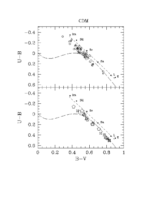
Figure 15: Color-color diagram for galaxies brighter than $M_{B}\leq-16$ in the CDM simulations. The long-dashed line represents the UBV position for main-sequence stars of luminosity class V. The short-dashed line provides a reference for galaxies. Along this line, galaxies of different morphological types are indicated in the position corresponding to their average colors. Upper panel: galaxies with $M\leq 3\times 10^{11}M_{\odot}$; lower panel: galaxies with $M>3\times 10^{11}M_{\odot}$. Galaxies located in environments of ambient density $\langle\rho\rangle/\bar{\rho}_{dm}>30$ are denoted by stars; those with $10<\langle\rho\rangle/\bar{\rho}_{dm}\leq 30$ are indicated by pentagons, those with $3<\langle\rho\rangle/\bar{\rho}_{dm}\leq 10$ by triangles, and those with $\langle\rho\rangle/\bar{\rho}_{dm}\leq 3$ by circles.

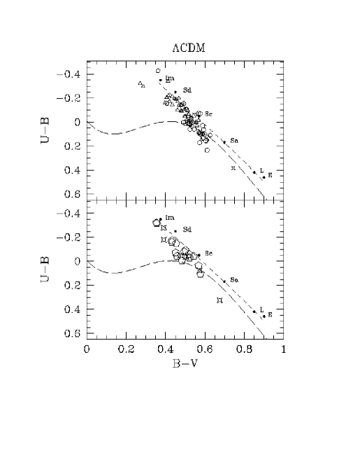
Figure 16: Color-color diagram for galaxies brighter than $M_{B}\leq-16$ in the $\Lambda$CDM simulations. Panels and symbols as in Fig. 15.

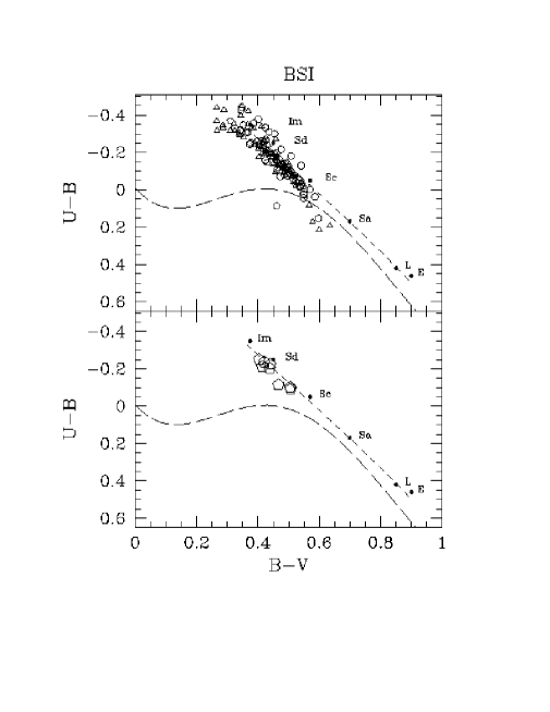
Figure 17: Color-color diagram for galaxies brighter than $M_{B}\leq-16$ in the BSI simulations. Panels and symbols as in Fig. 15.

Figs. (15), (16) and (17) are color-color diagrams ($U-B\;vs.\;B-V$) for galactic halos compiled from all the simulations in the respective scenarios. Only galaxies with $M_{B}\leq-16$ are plotted. The upper panels show galaxies of mass $M\leq 3\times 10^{11}M_{\odot}$, represented by different symbols according to the density of their environment. The lower panels show galaxies of mass $M>3\times 10^{11}M_{\odot}$. The long-dashed (lower) curve represents the main sequence for stars of luminosity class V. The short-dashed line represents colors of galaxies with different Hubble morphological sequence index, $T$, originally introduced by de Vaucouleurs & de Vaucoleurs [1964] in the First Reference Catalogue of Bright Galaxies (RC1). It ranges from $+10$ (irregulars) at the upper left to $-6$ (E0) at the lower right. Along this line, galaxies of different morphological types are indicated in the position corresponding to their average colors computed from the RC3 catalogue [de Vaucouleurs et al 1991]. The dispersion of color indices for galaxies of different morphological type ranges from 0.04, for ellipticals ($T=-5$) up to 0.1, for the irregulars ($T=10$). (See Buta et al [1994] for further details).

In the CDM scenario (Fig. (15)) we obtain a correlation between ambient density and morphology. For the more massive objects, (lower panel) lenticular and elliptical galaxies tend to be generated in environments of ambient density $\langle\rho\rangle_{50}>30\bar{\rho}_{dm}$. These objects are relatively isolated from other bright halos, having formed from coalescencing smaller halos. The relationships as simulated dynamically are thus consistent with the picture of generation of elliptical galaxies from spirals.

The rest of the halos are distributed along the line associated with various morphologies: in regions of elevated density ($10<\langle\rho\rangle_{50}/\bar{\rho}_{dm}\leq 30$; pentagons in the lower panel) one finds mostly massive spirals and hardly any irregulars. In the upper panel, less massive galaxies predominate in low-density environments ($\langle\rho\rangle_{50}/\bar{\rho}_{dm}\leq 3$), characterized by spiral morphology. There are also low-mass irregulars, but note that these are often located in intermediate or high-density environments ($10<\langle\rho\rangle_{50}/\bar{\rho}_{dm}\leq 30$).

The $\Lambda$CDM scenario (Fig. (16)) does not lead to lenticular or elliptical galaxies within the range of ambient densities obtained here (corresponding to groups of galaxies). This is not necessarily a shortcoming of the scenario, but could simply be a consequence of our limited dynamical simulation range. However, in contrast to CDM, it does yield massive irregular galaxies, while spirals predominate. The low-mass halos are also located in low-density environments, with spirals predominating. The absence of ellipticals and spirals of type $Sa$ may be attributed to the lower merger rate of halos in $\Lambda$CDM compared to CDM. This fact implies that the probability of finding field ellipticals in $\Lambda$CDM is much lower than in CDM. In order to be able to simulate ellipticals in $\Lambda$CDM, one would need to model larger volumes containing some regions of higher ambient density.

Another peculiarity of $\Lambda$CDM is a greater tendency for blue galaxies, contrary to what one might initially expect from a scenario with cosmological constant, if galaxies have had more time to evolve and thus become redder. Recall however, that here the parameters of each cosmological scenario have been chosen to yield an age of the universe similar to the CDM case ($\sim 13\times 10^{9}$ years) and a comparable time for evolution of galaxies. We will explain the relative redness of the CDM galaxy sample in section 4.3.

Finally, the BSI scenario Fig. (17) gives galaxies that are more concentrated in the blue regime. There is an excess of irregulars. Now, in the box simulated here, halo environments denser than $20\bar{\rho}_{dm}$ (Fig. (14)) are not realized in BSI as a result of the lower spectral amplitude. (Such environments could be realized in BSI if much larger scales were simulated.) As a consequence, ellipticals are not formed in simulations on this scale.

Earlier, we remarked that BSI as realized in a small box resembles an earlier stage of CDM. One consequence is that spiral galaxies of BSI located in regions of intermediate ambient density (pentagons in the lower panel) would presumably evolve further and end up as ellipticals and lenticulars, thus resembling the presently found CDM structures. Another way of looking at this point is that in a true BSI universe there would be some dense regions due to nonlinear effects on much larger scales, and in these regions the evolution could proceed on a timescale comparable to that of the CDM models realized here. Hence, it is reasonable to suppose that a true BSI universe would indeed produce ellipticals in dense regions at present.

In spite of these trends, the theoretical MD relationships emerging from our simulations are not as simple as might be inferred from the above remarks. For example, returning to Fig. (15) one can appreciate the quite diverse morphologies produced according to the CDM scenario in high-density environments, ranging from $Sd$ spirals to ellipticals. Thus, in addition to reproducing known trends quite naturally, our model appears capable of generating the complexity of conditions required for producing galaxies with a range of morphological characteristics. Because of the close relationship between morphology and star formation, we will now look more closely at the dependence of star formation on the environment, in order to understand the MD relationship in more detail.

4.3 Dependence of the star formation rate on environment

The influence of the ambient density on the star formation rate (SFR) is not yet well understood. At least two effects influencing the SFR in high-density regions are conceivable [Maia et al. 1994]. On the one hand, the SFR could be enhanced by tidal interactions triggering star formation, possibly in the form of bursts [Bushouse 1986, Kennicutt et al. 1987]. On the other hand, in the very high density regions in the core of clusters, close galaxy encounters lead to a depletion of interstellar gas and thus preferentially leave anemic spirals in clusters of galaxies [Dressler 1984].

The range of densities obtained for our numerical galaxies corresponds to the environment of field galaxies up to small groups at the high end. In addition, as mentioned earlier, close encounters, galactic cannibalism, and merging of systems of comparable mass are frequently encountered processes in the simulations reported here (see Figs.(3) and (4)). Hence, our study allows analysis of the SFR in an environmental situation of low density and frequent galaxy encounters.

Figure 18: Redshift evolution of the Star Formation Rate for halos found in all CDM simulations. Left column: galaxies with $M\leq 3\times 10^{11}M_{\odot}$. Right column: galaxies with $M>3\times 10^{11}M_{\odot}$. Each column is divided depending upon the density of the environments where galaxies are located: low density ($\langle\rho\rangle_{50}/\bar{\rho}_{dm}\leq 10$), medium density ($10<\langle\rho\rangle_{50}/\bar{\rho}_{dm}\leq 30$) and high density ($\langle\rho\rangle_{50}/\bar{\rho}_{dm}>30$). Only galaxies with $M_{B}\leq-16$ are plotted.

Figure 19: Same as in Fig. 18 but for the $\Lambda$CDM simulations.

In Figures (18) and (19) , the evolution with redshift of the SFR for bright ($M_{B}\leq-16$) halos found in all simulations for the CDM and $\Lambda$CDM models is presented. The graphics in the left hand column correspond to galaxies with masses $M\leq 3\times 10^{11}M_{\odot}$, while those with $M>3\times 10^{11}M_{\odot}$ are shown in the right hand column. These groups of galaxies have been subdivided in turn into three groups according to the ambient density at their location: in environments of low density ($\langle\rho\rangle_{50}/\bar{\rho}_{dm}\leq 10$), medium density ($10<\langle\rho\rangle_{50}/\bar{\rho}_{dm}\leq 30$) and high density $\langle\rho\rangle_{50}/\bar{\rho}_{dm}>30$, (upper, middle, and lower panels, respectively).

Note that this classification according to the environment takes into account the value of the density of material surrounding the galaxy at the current epoch (z=0), whereas the true density at the redshifts for which the SFR is plotted is not available. Thus, the current density is used as a surrogate for the density at the time of star formation and obviously is not a perfect indicator.

As shown in Figures (18) and (19), the SFR’s of the least massive halos do not exhibit any clearly defined correlation with their environment. A plausible explanation is that the SFR of less-massive halos depends mainly on their capacity to hold on to the gas, since there are several competing processes that can inhibit or stimulate star formation. Since these various processes have comparable magnitudes, it is not surprising that there are no clear trends in the dependence of the SFR on environment in less massive halos.

In contrast, for massive halos ($M>3\times 10^{11}M_{\odot}$ ) in CDM simulations, a drop of the SFR from $z\approx 1$ to $z=0$ is clearly seen. This drop is steeper for halos located in higher-density environments. A drop is also seen in $\Lambda$CDM simulations, albeit less pronounced. Typically, this drop in the star formation rate was associated with an apparent depletion of the cold gas available for star formation in the central regions of the halos. The dynamics of the supply of cold gas are complicated due to the supernovae feedback loop: Cold gas can be depleted if cooling is too slow compared with heating processes. Mergers tend to supply additional heat to the gas in the form of shocks. Hence one explanation for the star formation drop could be the increased frequency of mergers, which are characteristic for this period of evolution (see Fig. (6)). As we have seen in the course of this paper, in the CDM model the collapse rate is larger than in $\Lambda$CDM, which explains the difference in the degree of decrease in the SFR among the models and the larger number of reddened galaxies predicted by the CDM model, as we saw in Section 4.2.

4.4 Possible dependence of the Tully-Fisher relation on environment

The empirical relationship between luminosity and line width of spiral galaxies [Tully and Fisher 1977, Pierce and Tully 1988, 1992] is one of the most useful tools in cosmology, most notably when applied to modeling of large-scale velocity fields and to determination of the Hubble constant (see, e.g., Strauss & Willick [1995]).

There is some evidence supporting the existence of a ”universal” TF relation for field and cluster galaxies. Bothun et al [1984]; Richter and Huchtmeier [1984]; Giuricin et al [1986] and Biviano et al [1990] did not observe any dependence of the exponent of the TF relation in environments ranging from cluster to field galaxies. However, it is difficult to exclude the possibility of various systematic biases such as hidden dependence on environment [Pierce and Tully 1988, 1992].

Table 2: Parameters of the linear fits ($a$, $b$) and correlation coefficients ($r$) for the residuals of the Magnitude-Circular velocity relation in different luminosity bands as a function of the color indices of the numerical galaxies.

			a				b				r
Model	CI		B	R	I		B	R	I		B	R	I
	$U-B$		1.36	0.76	0.64		-0.08	-0.05	-0.04		0.58	0.42	0.38
CDM
	$B-I$		1.34	0.77	0.66		-2.35	-1.34	-1.15		0.64	0.47	0.42
	$U-B$		1.98	1.25	1.01		0.11	0.05	0.05		0.68	0.54	0.50
$\Lambda$CDM
	$B-I$		2.17	1.41	1.24		-3.56	-2.32	-2.05		0.76	0.62	0.58
	$U-B$		1.63	0.83	0.65		0.30	0.15	0.11		0.61	0.40	0.34
BSI
	$B-I$		1.89	1.08	0.89		-2.89	-1.65	-1.36		0.79	0.59	0.52

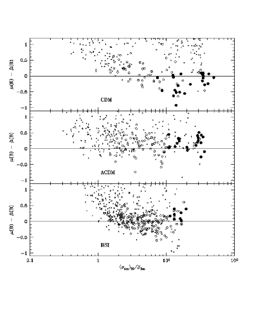
Figure 20: Residuals, after correcting by color effect (see text), of the magnitude-circular velocity relation in the B band as a function of the ambient overdensity $<\rho_{dm}>_{0.5}/\bar{\rho}_{dm}$. Galaxies with $M\geq 3\times 10^{11}M_{\odot}$ are denoted with dark hexagons, open circles represent halos with $3\times 10^{10}M_{\odot}<M<3\times 10^{11}M_{\odot}$ and crosses indicate faint halos with $M_{B}>-16$ y $M\leq 3\times 10^{10}M_{\odot}$ (not taken into account in the fits).

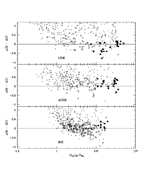
Figure 21: Same as in Fig. 20 but for the I band.

Hence, the universality of the Tully-Fisher (TF) relation remains an open question. If present, environmental bias in distance determination could have important consequences for mapping the large-scale velocity field. In view of the importance of this relation in cosmology and the difficulty of ascertaining the universality by empirical studies (which must rely on adequate statistics), a theoretical prediction of invariance or expected bias would be quite useful.

Using the numerical galaxies formed in our simulations, we have derived theoretical relations analogous to the observed Tully-Fisher (TF) relations in various photometric bands, for the three different cosmological models We found that the observed slopes, zero-points, and scatter of the TF relations are reproduced with reasonable accuracy by models with a cosmological constant ($\Lambda$CDM) or models with broken scale invariance (BSI) , while standard unbiased CDM leads to different slopes and/or zero points of the relation [Elizondo 1996, Elizondo et al. 1998].

In order to derive a theoretical TF relation, it is necessary to model the circular velocity of our numerical galaxies. Unfortunately, the spatial resolution of 39 kpc does not permit an accurate estimate of rotational velocities directly from the simulation data. Therefore, we devised an operational procedure for assigning “rotational velocities”, defined by the depth of the gravitational potential: $v_{\rm grav}=\sqrt{GM/r}$, where $M$ is the total mass of a galaxy within its assigned radius $r$ (1 or 2 cells, i.e. 39 or 78 kpc). We have tested this procedure for internal consistency with other indicators as reported in [Elizondo et al. 1998]. In addition, we find that the simulated TF relation for our galaxies is stable with respect to variations in the details of the halo finding algorithm used and changes in the spatial resolution of the simulations. The resolution check was carried out by comparing the $256^{3}$ and $128^{3}$ $\Lambda$CDM simulations reported in Section 2.5). Hence, we can be reasonably confident that our results primarily reflect the implications of our model for galaxies rather than the details of the numerical procedures used here.

In this section, we continue our study of environmental effects by searching for a significant dependence of the luminosity-line width relation on environment in a statistical sample of halos obtained in our simulations. More precisely, we have performed a stepwise linear regression of luminosity on rotational velocity, color index, and environment (characterized as above by the ambient overdensity)

We first consider residuals to the best fits to the TF relation in the B and I bands (i.e., $\hat{M}$): The residuals of the B-band and, to a lesser degree, the R-band and I-band TF - relations were found to be correlated with color index [$CI=(B-I)$ or $CI=(U-B)$] according to a relation of the form $\mu(M)\equiv M-\hat{M}=aCI+b$ , in agreement with Giraud [1986], who has found evidence for a color dependence of the difference in distance moduli derived from the TF - relation in two different bands. The fit parameters $a$ and $b$ as well as the correlation coefficients $r$ are listed in Table (2). Note that only galaxies with $B<-16$ are included in the fit, as before.

A hypothesis test of significant regression was performed by constructing the F–statistic for every fit. The null hypothesis $a=0$ was ruled out at the 99 % confidence level for all fits. As expected, the color dependence is least pronounced (but still significant) in all scenarios in the I - band. The slopes of the $\mu(M)$ vs. CI - relation are different for different cosmological scenarios. In all scenarios, the slope of the relation is positive. Thus, the trend is for bluer galaxies to be brighter than predicted by the uncorrected TF - relation.

Having thus obtained a color-corrected TF-relation, we now compute the residuals with respect to the corrected relation in these two bands and search for a relationship between these residuals and the ambient overdensity $<\rho_{dm}>_{0.5}/\bar{\rho}_{dm}$ as defined earlier. The regressions are performed separately for each scenario using all galaxies in the corresponding catalog. After removing the color trend as above, regression on the remaining residuals was thus performed according to the model $\mu(M)-\hat{\mu}(M)=c\log(<\rho_{dm}>_{0.5}/\bar{\rho}_{dm})+d$. (Here $\hat{\mu}(M)$ is the residual predicted using the color regression as above.) In Fig. (20) and (21) the B and I band residuals $\mu(M)-\hat{\mu}(M)$ is plotted as a function of the ambient overdensity $<\rho_{dm}>_{0.5}/\bar{\rho}_{dm}$ of dark matter. We have also applied the hypothesis test of regression by means of the F-statistic to these plots. Within the dynamical range studied here, there was no environmental effect ($c=0$) in the TF at the 99 % or even 95 % confidence levels in BSI or $\Lambda$CDM. However, at the 99 % confidence level there was an environmental effect in the CDM sample: in the I-band, we find $c=-0.21$, $d=0.18$ and in the B-band, $c=-0.36$, $d=0.33$. Qualitatively similar results are obtained if $\mu(M)$ is modeled (residuals without color correction) instead of $\mu(M)-\hat{\mu}(M)$.

Our results for the $\Lambda$CDM and BSI scenarios are consistent with the usual view that the TF - relation is unbiased with respect to environment. However, despite the fact that we find a statistically significant environmental dependence of the residuals on environment in our CDM sample, it would not be correct to infer that the TF -relation for spirals would have environmental bias in a CDM universe: the entire statistical effect could be due to inclusion of the “ellipticals”, classified here on the basis of colors, as was discussed in Section 4.2. Indeed, once the “elliptical” galaxies are removed from the fit, we find, at a 99% confidence level, no environmental effect on the TF relation for CDM either.

5 Discussion and conclusions

We have presented results of cosmological hydrodynamical simulations incorporating a multiphase model of the ISM, radiative cooling, star formation, metal enrichment, and supernova feedback. The simulations have been performed for three cosmological scenarios: CDM, $\Lambda$CDM and BSI.

The depth of modeling of the physical processes in the baryonic component has permitted us to study the motion and evolution of gas inside and around dark matter halos. As described in § 3.3, the gas flow is extremely complicated: While we clearly see accretion shocks at large distances from halos (up to 1 Mpc), the flow inside the shock cannot be treated as spherical. A fraction of the gas flows along filaments. It penetrates very deeply inside the “caverns” which are produced by accretion shocks. We frequently found outflows of gas inside caverns. These outflows (“chimneys”) are not directly related with the supernova feedback, but in some cases are enhanced by it. The distribution of the gas is very much affected by the short-scale processes related with the star-formation and its back-reactions to the surrounding gas. In particular, metal enrichment change the position of the accretion shock. The higher cooling rate for a metal enriched gas causes it to produce more cold clouds and weaker pressure gradients. Therefore, star formation is more efficient, and galaxies become brighter and bluer.

We have also analyzed the effects of environment on the observational properties of our numerical galaxies, such as morphologies (as characterized by colors), SFR and Tully-Fisher relation. We can summarize the main results as follows:

• The percentages of galaxies with different morphologies differ markedly from one scenario to another. Concretely, the CDM simulations produce a considerable population of elliptical galaxies ($\sim 13$%) with red colors and a dearth of irregulars ($\sim 3$ %) at the range of densities (in a 0.5 Mpc scale) studied here, corresponding to the typical environments of loose groups and field galaxies. $\Lambda$CDM simulations produce fewer red ellipticals, ($\sim 2$ %) while BSI produces very blue galaxies dominated by spiral ($\sim 80$%) and irregular ($\sim 20$%) types. Differences between the morphology distributions produced in different scenarios persist even if the ambient density is held constant.

• The SFR history for massive halos ($M>3\times 10^{11}M_{\odot}$) exhibit a drop from $z\simeq 1$ to $z=0$. This drop in the SFR is more pronounced in halos located in higher density environments. But, for the same range of environment densities, the drop is larger for halos found in CDM simulations than in $\Lambda$CDM. On the contrary, the SFR history of less massive halos ($M<3\times 10^{11}M_{\odot}$) does not exhibit a clearly defined correlation with the ambient density at present epoch.

• The Tully-Fisher relation for the galaxies in $\Lambda$CDM and BSI simulations does not depend on environment, with a 99% confidence level. For CDM, we find a statistically significant environmental dependence of the TF-relation, but this effect is due to the inclusion of “ellipticals”, that are produced in this model. When the “ellipticals” are removed from the sample, we find no environmental effect, at a 99% confidence level as in the other models.

We conclude that the ambient density is NOT the only factor defining observable galaxy properties. The merging history, tidal encounters, and interactions with the surrounding gaseous medium could be important in determining the properties of galaxies [Balland et al. 1997] located in regions of similar ambient density. Our simulation technique provides a point of departure for such a study, since a representative sample of possible initial conditions can be generated by different realizations.

We have also shown that a proper description of physical processes in the baryonic component is important in modeling the formation and evolution of galaxies and in predicting their observational properties. We are still far from a complete understanding, let alone modeling, of the physical processes that govern the formation and evolution of galaxies. Nonetheless, the YK³ code takes into account mechanisms corresponding to physical processes which according to numerous lines of evidence are most important in the dynamics of galaxies. The modeling of these processes incorporates the available physical and astrophysical knowledge to the depth possible consistent with computational limitations and the need to minimize the number of degrees of freedom in the parametrization. As a general principle, predictive power is strongly improved by parsimonious use of fitting parameters, and indeed the ability to make predictions is the difference between modeling and curve fitting.

Improvements in numerical resolution would certainly be useful in order to extend our results of the effects of environment to larger-scale structures. Clearly, on the basis of the present results one cannot exclude additional environmental effects that could result from the existence of structures on scales beyond our current box size (5 Mpc). Nevertheless, we can conclude that our numerical model for galaxy formation, which includes the most relevant physical processes for the baryonic component, is capable of reproducing most of the observational trends of real galaxies. We have seen that for a reasonable expenditure of computational resources, it is possible to study problems such as environmental effects while including hydrodynamics. Hence, the combination of hydrodynamical simulations with modeling of the baryonic component constitutes a very useful and powerful tool for investigating the complex phenomena of galaxy formation.

References

- Balland et al. 1997 Balland, C., Silk, J. and R. Schaeffer, 1997, astro-ph/9711036.
- Baugh et al 1997 Baugh, C.M., Cole,S., Frenk, C.S. and Lacey, C.G. 1997, astro-ph/9703111.
- 1990 Biviano, A., Giuricin, G., Mardirossian, F. and Mezzetti, M., 1990 ApJS 74 325
- 1984 Bothun, G., Aaronson, M., Schommer, R.A., Huchra, J. and Mould, J.R., 1984 ApJ 278 475
- 1996 Bond, J. R., Kofman, L. and Pogosian, D., 1996, Nature 380 603
- Bruzual and Charlot 1993 Bruzual, G. and Charlot, S., 1993 ApJ 405 538
- Bushouse 1986 Bushouse, H.A., 1986 ApJ 91 255
- 1994 Buta, R, Mitra, S, de Vaucouleours, G & Corwin Jr., H. G., 1994 ApJ 107 118
- Cen et al. 1990 Cen, R.Y., Jameson, A., Liu, F. y Ostriker, J.P., 1990 ApJ 326 41
- Cole et al. 1994 Cole, S.J., Aragón-salamanca, A., Frenk, C.S., Navarro, J.F. and Zepf, S.E., 1994 MNRAS 271 781
- Colella and Woodward 1984 Colella, P. and Woodward, P. R., 1984, J.Comp.Phys, 54, 174
- 1964 de Vacouleurs, G & de Vaucouleurs, A., 1964, Reference Catalogue of Bright Galaxies, University of Texas Monographs in Astronomy, No 1 (University of Texas Press, Austin)
- de Vaucouleurs et al 1991 de Vaucouleurs, G., de Vaucouleurs, A. and Corwin Jr., H. G., Buta, R. J. 1991, Paturel, G & Fouque, P., 1991, Third Reference Catalogue of Bright Galaxies (RC3), Springer-Verlag
- Dressler 1980 Dressler, A., 1980 ApJ 236 351
- Dressler 1984 Dressler, A., 1984, ARA&A, 22, 185
- Elizondo 1996 Elizondo, D., 1996, PhD thesis, Universidad Autónoma de Madrid. (Spain)
- Elizondo et al. 1998 Elizondo, D., Yepes, G., Kates, R., Müller, V. and Klypin, A., 1998 ApJ. (Submitted)
- Evrard 1988 Evrard, A.E., 1988 MNRAS 235 911
- 1986 Giraud, E.H., 1986 A&A 155 283
- Giroux and Shapiro 1986 Giroux, M and Shapiro, I., 1986 ApJS 102 191
- 1986 Giuricin, G., Mardirossian, F. and Mezzetti, M. 1986 A&A 157 400
- Heyl et al. 1995 Heyl, J.S., Cole, S., Frenk, C.S. and Navarro, J.F., 1995 MNRAS 274 755
- Hubble and Humason 1931 Hubble, E. and Humason, M.L. 1931 ApJ 74 43
- Kaiser 1984 Kaiser, N. 1984 ApJ 284 L9
- Kates et al 1995 Kates, R., Müller, V., Gottlöber, S., Mücket, J. P., and Retzlaff, J., 1995 MNRAS 277 1254
- Katz and Gunn 1991 Katz, N. and Gunn, J.E., 1991 ApJ 377 365
- Kauffmann et al. 1993 Kauffmann, G., White, S.D.M. y Guiderdoni, B., 1993 MNRAS 264 201
- Kennicutt et al. 1987 Kennicut, R.C., Keel, W.C., van der Hulst, J.M., Hummel, E., and Roettiger, K.A., 1987 ApJ 93 1011
- Lacey and Cole 1993 Lacey, C. and Cole, S., 1993 MNRAS 262 627
- Maia et al. 1994 Maia, M. A. G., Pastoriza, M. G., Bica, E., and Dottori, H., 1994 ApJS 93 425
- McKee and Ostriker 1977 McKee, C.F. and Ostriker, J.P., 1977 ApJ 218 148
- Mücket et al. 1996 Mücket, J.P., Petitjan, P., Kates, R. and Riediger, R., 1996 A&A 308 17
- Mücket and Kates 1997 Mücket, J.P and Kates, R., 1997 A&A 324 1
- Oemler 1974 Oemler, A., 1974 ApJ 194 1
- Peebles 1980 Peebles, P.J.E., 1980, The Large-Scale Structure of the Universe (Princeton, Princeton University Press)
- Petitjean et al. 1995 Petitjean, P., Mücket, J., Kates, R., 1995 A&A 295 L9
- Petitjean et al. 1996 Petitjean, P., Pecontel, E., Valls-Gabaud, D. and Charlot, S. 1996, Nature 380 411
- Pierce and Tully 1988 Pierce, M.J. and Tully, R.B., 1988 ApJ 330 579
- 1992 Pierce, M.J. and Tully, R.B., 1992 ApJ 387 47
- 1984 Richter, O.G. and Huchtmeier, W.K., 1984 A&A 132 253
- Smith et al. 1993 Smith, M.S., Kawano, L.H. and Malaney, R.A., 1993 ApJS 85 219
- Schweizer 1986 Schweizer, F., 1986, Science 231 227
- 1995 Strauss, M.A. and Willick, J.A., 1995 , Phys. Rep. 261, 271
- Tully and Fisher 1977 Tully, R.B. and Fisher. J.R., 1977 A&A 54 661
- White and Frenk 1991 White, S.D.M. and Frenk, C.S., 1991 ApJ 379 52
- Whitmore 1990 Whitmore, B.C., 1990, Clusters of Galaxies. W.R. Oegerle, M.J. Fitchett and L. Danly eds. Cambridge Univ. Press, p.139
- 1997 Yepes, G., Kates, R., Khokhlov, A., & Klypin, A., 1997 MNRAS 284 235 (YK3)
- 1997 Yepes G., 1997, ASP Conf. Series 126 279.
- Yepes and Elizondo 1997 Yepes, G. & Elizondo D., 1997, Proceedings of the XII International Potsdam Workshop on Large Scale Structure in the Universe, V. Müller, J. Mücket and S. Gottlöber eds, World Scientifc, in press.