Cosmological Consequences of String-forming Open Inflation Models

Abstract

We present a study of open inflation cosmological scenarios in which cosmic strings form betwen the two inflationary epochs. It is shown that in these models strings are stretched outside the horizon due to the inflationary expansion but must necessarily re-enter the horizon before the epoch of equal matter and radiation densities. We determine the power spectrum of cold dark matter perturbations in these hybrid models, finding good agreement with observations for values of $\Gamma=\Omega_{0}h\sim 0.3$ and comparable contributions from the active and passive sources to the CMB. Finally, we briefly discuss other cosmological consequences of these models.

I Introduction

Over the last two decades, two paradigms have emerged as possible explanations for the origin of the cosmological structures seen today. Inflationary models [1], originally developed with the aim of solving the horizon and flatness problems, were soon seen to generate a spectrum of quantum-mechanical fluctuations with an approximately scale-invariant (Harrison-Zel’dovich) form. On the other hand, cosmic strings [2] are topological defects which may have formed at cosmological phase transitions, and since their late-time evolution is scale-invariant they to can produce a scale-invariant spectrum of perturbations.

These two paradigms are usually considered to be incompatible with each other, the argument being roughly that any strings formed before or during inflation will be stretched to unobservable scales, and any strings formed afterwards will be too light to have any cosmological relevance (at least, from the point of view of structure formation).

Recently, however, theoretical cosmologists have realized (aided, undoubtedly, by their observational counterparts [3]) that inflation does not necessarily produce a critical-density universe, and in fact inflationary models can now be built that produce any value of $\Omega_{0}$ (subject to some model-dependent amount of fine-tuning) [4, 5]. In particular, there has been recent interest in models where an open universe is produced as a result of two epochs of inflation, and it has been suggested that in such models cosmic strings can form between the these two epochs [7].

Here we present a study of the cosmological consequences of these models. Since the second inflationary period is rather short, it does not necessarily follow that they will be unobservable by the present day. In fact, it will be shown that in these models strings must necessarily re-enter the horizon before the epoch of equal matter and radiation densities. This means that they can still play a crucial cosmological role, namely in the formation of structures in the universe. Note that these will therefore be hybrid structure formation models, with perturbations being generated by both active and passive sources.

We will start by reviewing the key concepts behind open inflation in section II. Following this we discuss cosmic string evolution in these models (section III) and calculate the corresponding total CDM power spectrum (section IV). Finally, we briefly discuss other cosmological consequences of these models and present our conclusions. Throughout this paper we have chosen units such that the speed of light is unity, $c=1$, and adopted the convention $H_{o}\equiv 100\,h\,{\rm km}\,{\rm sec}^{-1}\,{\rm Mpc}^{-1}$.

II Basics of Open Inflation

Open inflation models can be roughly described as a period of old inflation followed by a period of new inflation [4, 5]. One starts with a scalar field trapped in false vacuum. The potential barrier must be high enough for the corresponding decay rate to be exponentially suppressed. This is required for the universe to expand enough for bubble nucleation to occur in a smooth de Sitter spacetime background. Additionally, this ensures that the probability of collision between two bubbles is small enough for the universe to survive up to the present day.

In these circumstances, the interior of the bubble will be a homogeneous and isotropic universe (thus solving the horizon problem) with negative spatial curvature. Then the inflaton starts rolling down the potential, preserving homogeneity and isotropy, and as it approaches the true minimum its oscillations will reheat the universe and leave it in the usual radiation-doinated epoch. The value of the present density of the universe will be determined by the duration of this second inflationary period, which is in turn determined by the initial value of the inflaton.

Note that the two periods of inflation may [4] or may not [5] be driven by the same scalar field. In the latter case the first inflationary epoch will be due to a ‘heavy’ inflaton with a steep potential barrier, while in the second epoch a ‘light’ inflaton rolls in a nearly-flat direction orthogonal to that of the original tunnelling. Also, in the latter case we will typically have an ensemble of very large (but finite) ’inflationary islands’ [6] rather than an infinite open universe. While the specific particle-physics details of the two classes of models will of course be different, their basic cosmological features (to be summarized below) are nevertheless very similar. Hence, for simplicity we will be concentrating on the model by Bucher et al. [4] in the remainder of this paper.

Now, the metric inside the nucleated bubble has the usual Friedmann-Robertson-Walker (FRW) form

$$ds^{2}=-dt^{2}+a^{2}(t)\left[d\zeta^{2}+\sinh^{2}(\zeta)d\Omega_{2}^{2}\right]\,,$$ (1)

where $d\Omega_{2}^{2}=d\theta^{2}+\sin^{2}\theta d\phi^{2}$. Then the corresponding Friedmann and inflaton equations are

$$H^{2}=\left(\frac{\dot{a}}{a}\right)^{2}=\frac{1}{a^{2}}+\frac{8\pi}{3m_{Pl}^{2}}\left(\frac{1}{2}\dot{\phi}^{2}+V(\phi)\right)\,,$$ (2)

$$\ddot{\phi}+3H\dot{\phi}=-\frac{\partial V}{\partial\phi}\,.$$ (3)

We will take the potential to be of the generic form

$$V(\phi)=\frac{\lambda\phi^{n}}{nm_{Pl}^{n-4}}\,.$$ (4)

but for definiteness we will generally use $n=2$ in the following sections. It can be shown [4] that for given choices of $n$, the temperature of reheating (denoted $T_{r}$) and the cosmological parameters $\Omega_{0}$ and $h$, the appropriate open inflationary model has an initial value of the inflaton given by

$$f^{2}\equiv\left(\frac{\phi}{m_{Pl}}\right)^{2}_{i}=\frac{n}{8\pi}\left[49.48+\ln{\left(\frac{T_{r}(GeV)^{2}}{h^{2}(1-\Omega_{0})}\right)}\right]\,.$$ (5)

It is fairly straightforward to see that there are two evolution regimes for the above equations. At early times, spatial curvature will be dominant, so we have $a\propto t$ and $\Omega\simeq 0$. Then the second epoch of inflation will set in, and the scale factor will approximately evolve as $a\propto\exp{(t)}$, with $\Omega$ being driven to a value very close to unity. The transition between these two regimes happens at a time $t_{t}$ given by

$$\frac{t_{r}}{t_{t}}=1+\frac{4\pi f^{2}}{n}=N\,,$$ (6)

where $t_{r}$ is the epoch corresponding to the reheating temperature $T_{r}$. Note that this ratio is also the number of e-foldings N in the model. As the inflaton approaches its true minimum, reheating takes place. We will assume that this happens instantaneously, and therefore the universe rapidly becomes radiation-dominated, with the scale factor growing as $a\propto t^{1/2}$. By numerically studying equations (2) and (3), one can show that the following analytic expression provides a reasonably accurate description of the evolution of the scale factor

$$a(t)=\cases{\frac{t}{t_{Pl}}&for $t<t_{t}$\cr\frac{t_{t}}{t_{Pl}}{\rm exp}\left(\frac{t}{t_{t}}-1\right)&for $t_{t}<t<t_{r}$\cr\frac{t_{t}}{t_{Pl}}{\rm exp}\left(\frac{t_{r}}{t_{t}}-1\right)\left(1+2\frac{t-t_{r}}{t_{t}}\right)^{1/2}&for $t_{r}<t<t_{eq}$}\,.$$ (7)

The Hubble length has the form

$$H(t)^{-1}=\cases{t&for $t<t_{t}$\cr t_{t}&for $t_{t}<t<t_{r}$\cr 2(t-t_{r})+t_{t}&for $t_{r}<t<t_{eq}$}\,.$$ (8)

These will therefore be used in the remainder of the paper.

III String Formation and Evolution

As discussed by Vilenkin [7], there are a number of reasonably natural mechanisms that could lead to string formation between the two inflationary epochs. Two simple exemples are the cases where a complex scalar field is coupled to the field responsible for the first inflationary epoch or to spatial curvature. Again we will not be discussing the individual details of each possible model but will instead focus on their generic cosmological properties.

The evolution of the cosmic string network will be described in the context of the quantitative analytic model introduced by Martins and Shellard [8] and extended to general FRW models in by the present authors [9]. Here we will briefly recall the essential features of this approach; the reader is referred to the above papers for a more detailed discussion (see also [10]).

The basic idea is to describe the string network by a small number of macroscopic (or ‘averaged’) quantities whose evolution equations are derived from the microscopic string equations of motion. In the simplest case, there are only two such quantities, the energy of a piece of string,

$$E=\mu a(\tau)\int\epsilon d\sigma\,,$$ (9)

($\epsilon$ being the coordinate energy per unit length on the string worldsheet), and the string root-mean squared (RMS) velocity, defined by

$$v^{2}=\frac{\int{\dot{\bf x}}^{2}\epsilon d\sigma}{\int\epsilon d\sigma}\,.$$ (10)

In passing, we point out that this kind of approach has been extended to more complicated models, which are suitable for describing cosmic strings containing significant small-scale strucutre (‘wiggles’) [10, 11] or superconducting currents [10, 12]. In the present case, however, the inflationary epoch will make any such effects less important than in more standard scenarios, so we will not explicitly consider them (however, see section IV).

Distinguishing between long (or ‘infinite’) strings and loops, and knowing that the former should be Brownian we can define the long-string correlation length as $\rho_{\infty}\equiv\mu/L^{2}$. A phenomenological term must then be included describing the interchange of energy between long strings and loops—a ‘loop chopping efficiency’, denoted ${\tilde{c}}$ and expected to be slightly smaller than unity. One can then derive the evolution equation for the correlation length $L$, which has the form [8, 9]

$$\frac{dL}{dt}=HL\left(1+\frac{v^{2}}{\left[1-(1-\Omega)(HL)^{2}\right]^{2}}\right)+\frac{{\tilde{c}}}{2}v\,.$$ (11)

Note that we do not include frictional forces due to particle scattering on strings [8], since for cosmic strings forming at or around the GUT scale these are subdominant after reheating.

One can also derive an evolution equation for the long string velocity with only a little more than Newton’s second law [8, 9]

$$\frac{dv}{dt}=\left[\left[1-(1-\Omega)(HL)^{2}\right]^{2}-v^{2}\right]\frac{{\tilde{k}}}{L}-2Hv\left(1-\frac{v^{2}}{\left[1-(1-\Omega)(HL)^{2}\right]^{2}}\right)\,;$$ (12)

here ${\tilde{k}}$ is another phenomenological parameter of order unity which specifies the relative importance of curvature and momentum in determining the dynamics of the strings [8]. These quantities are sufficient to quantitatively describe the large-scale properties a cosmic string network.

A simple analysis of the evolution equations (11)–(12) reveals the basic features of the evolution of a cosmic string network in these circumstances. Since we are mainly interessed in these strings as possible seeds for structure formation, we will assume later on that they are formed at an epoch such that they have a mass per unit length $G\mu\sim 10^{-6}$. It is fairly straightforward to generalize these results to other energy scales—see for exemple [8, 10]. Before the second inflationary period starts we have $\Omega\simeq 0$ and an approximate solution (meaning that it would be exact if $\Omega$ was exacly zero) is [13]

$$L(t)\propto t\left(\ln{t}\right)^{1/2}\,,$$ (13)

$$v(t)\propto\left(\ln{t}\right)^{-1/2}\,.$$ (14)

Hence, at the onset of the second inflationary epoch, strings will be fairly straight (having a correlation length close to the horizon) and non-relativistic. It is intuitively obvious that during inflation the strings will be conformally stretched, and indeed the solution of (11)–(12) in this case is

$$L(t)\propto\exp{\left(\frac{t}{t_{t}}\right)}\,,$$ (15)

$$v(t)\propto\exp{\left(-\frac{t}{t_{t}}\right)}\,.$$ (16)

Note that it is only during the second period of inflation (not before) that the strings are stretched outside the horizon. This fact is crucial for what follows.

It is easy to verify using the expressions for the evolution of the scale factor and Hubble parameter that if a given scale leaves the Hubble sphere at the time $t_{out}<t_{r}$ and re-enters it at the time $t_{in}\gg t_{r}$ then

$${a_{in}\over a_{r}}\times{a_{r}\over a_{out}}\sim{\left({{2t_{in}}\over t_{t}}\right)}^{1/2}\times{a_{r}\over a_{out}}\sim{{2t_{in}}\over t_{t}}\,,$$ (17)

which implies that

$${a_{in}\over a_{r}}\sim{a_{r}\over a_{out}}\,.$$ (18)

We also know that during inflation the importance of the curvature term decreases as

$$\Omega-1={k\over{a^{2}V}}\propto a^{-2}\,,$$ (19)

while during the radiation era we have

$$\Omega-1={k\over{a^{2}\rho_{rad}}}\propto a^{2}\,.$$ (20)

This implies that the value of $\Omega$ when the strings leave the horizon must be approximatelly the same to the value of the $\Omega$ when the strings re-enter the horizon. Consequently, since they leave during the second inflationary period, when the density is very close to critical, we can expect them to re-enter not much later than the epoch of equal radiation and matter densities. This can be confirmed as follows.

From the above discussion, we know that at the start of the radiation era the strings will have negligible velocity (as well as small-scale structure) and will continue to be conformally stretched, so that our averaged quantities now behave as

$$L(t)\propto t^{1/2}\,,$$ (21)

$$v(t)\propto t^{1/2}\,.$$ (22)

Notice the different behaviour of the string RMS velocity in the present case compared to the usual ‘stretching regime’ (where it behaves like $v\propto t$—see [8, 10]). This is because, as we pointed out above, in the present case the effect of the frictional force due to particle scattering on strings will be negligible. Obviously these solutions can be confirmed numerically (see below).

Now, the crucial observation is that this slow growth of the correlation length $L$ relative to $H^{-1}$ (which is proportional to time in the radiation era) means that strings can indeed get back inside the horizon in time to play a significant role in the formation of structures in the universe. As velocity grows the loop formation term will eventually become important, and the network will ‘switch’ to the linear scaling regime. In principle, one would require that strings should be back inside the horizon at the epoch of equal matter and radiation densities, $t_{eq}$. However, we note that it is also clear that some time will be necessary for the network to reach the usual linear scaling regime [8] once it is back inside the horizon. Hence one sees that this class of models will provide a rather natural way of generating ‘deviations from scaling’ near $t_{eq}$, which have been claimed [14] to be necessary to reconcile the cosmic string scenario with observation.

For the moment, we can estimate how much inflation can be tolerated by a cosmic string network that is requred to re-enter the horizon before $t_{eq}$. We require $H(t_{eq})^{-1}>L(t_{eq})$ to determine the amount of inflation which may occur and define $N$ to be the number of e-foldings in the second inflationary period. We assume for simplicity that the correlation length changes instantaneously from the exponential to the power-law growth laws. Also for simplicity, we temporarily consider the case where the second inflationary period starts at the moment when the strings form.

It is then a simple matter to show that the maximum number of e-foldings $N_{str}$ that a string network can tolerate in these circumstances is given by the solution to

$$N_{str}=\frac{1}{2}\left[\ln\left(4\frac{t_{eq}}{t_{t}}\right)+\ln\left(1+N_{str}\right)\right]\,.$$ (23)

On the other hand, the number of e-foldings $N_{inf}$ required for an open inflation model whose second period of inflation starts when the strings form to produce a present universe with a density $\Omega_{0}$ is

$$N_{inf}=\frac{1}{2}\left[49.48+\ln\left(\frac{0.301m_{Pl}^{2}}{h^{2}(1-\Omega_{0})}\frac{t_{Pl}}{t_{t}}\right)-\ln\left(1+N_{inf}\right)\right]\,.$$ (24)

These two quantities are plotted (for $h=0.7$ and two different values of $\Omega_{0}$) in figure 1. This confirms that strings will necessarily be back inside the horizon at $t_{eq}$ . Depending on initial conditions, they can actually return many orders of magnitude in time before that. Note that even though we assumed (for simplicity) that strings were formed at $t=t_{t}$, our result is completely general, since even if formed before strings can not leave the horizon until $t_{t}$. From this plot we can also see that $N_{str}$ is much more sensitive to the cosmological parameters than $N_{inf}$ (due to its dependence on $t_{eq}$). Furthermore, since $t_{eq}/t_{Pl}\propto\Omega_{0}^{-2}$, the smaller $\Omega_{0}$, the more comfortably strings will get back inside. In other words, the ’extreme’ case where strings just manage to get back inside the horizon at $t_{eq}$ happens for a critical density that is just below unity and for a reheat temperature that is as low as possible. This can be confirmed in figure 2, where we have summarized the cosmological evolution of some sample string networks.

IV Large Scale Structure

We assume that during the second period of inflation the following slow-roll conditions are satisfied:

$${\dot{\phi}}\sim-{1\over{3H}}V^{\prime},$$ (25)

$${\epsilon}\equiv{{m^{2}_{\rm pl}}\over{16\pi}}{\left({{V^{\prime}}\over V}\right)}^{2}\ll 1,$$ (26)

and

$${\eta}\equiv{{m^{2}_{\rm pl}}\over{8\pi}}{\left({{V^{\prime\prime}}\over V}\right)}\ll 1.$$ (27)

In this case the condition ${\dot{\phi}}^{2}\ll V$ is also verified and then

$${H^{2}}\sim{{8\pi V}\over{3m^{2}_{\rm pl}}}.$$ (28)

As we have seen before the initial value of the inflaton field can be chosen in such a way as to allow $\Omega_{0}$ to have any ’desired’ value below unit. Here, we start by reviewing the results for the spectrum of adiabatic fluctuations produced during the second stage of inflation subject to the three slow-roll conditions listed above in the case with $\Omega_{0}\sim 1$. We will then discuss how the power spectrum can be rescaled to allow for open models taking into account that scales $\mathrel{\hbox to0.0pt{\lower 4.0pt\hbox{\hskip 1.0pt$\sim$}\hss}\raise 1.0pt\hbox{$<$}}100h^{-1}{\rm Mpc}$ come inside the horizon when the curvature is still dynamically unimportant. For the sake of simplicity we will also take $h=1$ for the time being.

The power spectrum of the density contrast measured today of the adiabatic fluctuations produced during inflation in a flat universe with zero cosmological constant can be written as

$$S(k)=4\pi^{3}P(k)={\left(k\over{a_{0}H_{0}}\right)}^{4}T^{2}(k)A_{S}^{2}(k).$$ (29)

where $k$ is given in units of ${\rm Mpc}^{-1}$. The quantity $A_{S}^{2}(k)$ specifies the initial spectrum and can be calculated precisely in terms of the inflationary potential [17] as

$$A_{S}^{2}(k)={{32V}\over{75m^{4}_{\rm pl}}}\epsilon^{-1}\propto\lambda\left(\frac{\phi}{m_{Pl}}\right)^{n+2}.$$ (30)

The transfer function $T(k)$ for the CDM models considered here is accurately given by Bardeen et al. [19] as

$$T(k)={\ln(1+2.34k)\over{2.34k}}\times[1+3.89k+(16.1k)^{2}+(5.46k)^{4}+(6.71k)^{4}]^{-1/4}.$$ (31)

Having discussed the results in the simpler case with $\Omega_{0}=1$ we are now in a position to generalize these results for open universes. To do this we take into account that perturbations on the scales of interest to us, that is $\mathrel{\hbox to0.0pt{\lower 4.0pt\hbox{\hskip 1.0pt$\sim$}\hss}\raise 1.0pt\hbox{$<$}}100h^{-1}{\rm Mpc}$, were generated and re-enter the horizon when $\Omega$ is still very close to unity for any observationally reasonable choice of $\Omega_{0}$. Having established this, it is straightforward to rescale the spectrum for a flat universe with a zero cosmological constant in the following way :

$$S(k,h,\Omega_{0})=S(k,1,1)\cdot\Omega_{0}^{2}{h}^{4}\cdot g^{2}(\Omega_{0}),$$ (32)

where $k$ is in units of $\Omega_{0}h^{2}\,{\rm Mpc}^{-1}$, and $g(\Omega_{0})$ is given by [20]

$$g(\Omega_{0})=\frac{5\Omega_{0}}{2\left[\Omega_{0}^{4/7}+1+\Omega_{0}/2\right]}.$$ (33)

The factor $g(\Omega_{0})$ gives the supression of growth of density perturbations in an open universe relative to that of a flat universe with zero cosmological constant. Let us define the horizon crossing amplitude $\delta_{H}(k)$ as

$$\delta_{H}(k)=A_{S}(a_{0}H_{0})\times{{g(\Omega_{0})}\over\Omega_{0}}$$

This quantity is constrained by the four-year COBE data to be:

$$\delta_{H}(\Omega_{0})=1.95\Omega_{0}^{-0.35-0.19\ln\Omega_{0}}$$

if only inflationary perturbations are responsible by cosmic structure. This fit works to better than $2\%$ for $0.2\leq\Omega_{0}<1$ and the statistical uncertainty is $7\%$ [15]. The above normalization was obtained for an open model with a flat-space scale invariant spectrum instead of the open-bubble inflation model spectrum. However, for $0.3\leq\Omega_{0}<1$ these lead to different normalization for $\delta_{H}$ only by a factor smaller than $10\%$ [16].

Having characterized the spectrum of adiabatic fluctuations produced during the second stage of inflation we now proceed to study the power spectrum generated by the cosmic string network. Again we start by studying the simpler case of a $\Omega_{0}\sim 1$ universe and then generalize our results for open models as we did for the inflationary perturbations. We use the semi-analytic model of Albrecht and Stebbins [22] to estimate the power spectrum of density perturbations induced by cosmic strings. This is given by

$$P(k)=16\pi^{2}(1+z_{eq})^{2}\mu^{2}\int_{\tau_{i}}^{\infty}|T(k;\tau^{\prime})|^{2}{\cal F}(k\xi/a)d\tau^{\prime}$$ (34)

(35)

$${\cal F}(k\xi/a)={2\over\pi^{2}}{{\beta^{2}\Sigma}}{\chi^{2}\over\xi^{2}}\Big{(}1+2(k\chi/a)^{2}\Big{)}^{-1}.$$ (36)

In these equations, $a$ is the scale factor which evolves smoothly from radiation- to dust-dominated expansion, $\tau_{i}$ is the conformal time at which the string network formed, and $T(k,\tau^{\prime})$ is the transfer function for the evolution of the causally-compensated perturbations. The parameters used in the Albrecht-Stebbins estimate of the cosmic string power spectrum are given by

$$\xi\equiv(\rho_{L}/\mu)^{-1/2},\qquad\beta\equiv\langle v^{2}\rangle^{1/2},\qquad\Sigma\equiv{\mu_{r}\over\mu}\gamma_{b}\beta_{b}+{1\over 2\gamma_{b}\beta_{b}}\Big{(}{\mu_{r}^{2}-\mu^{2}\over\mu\mu_{r}}\Big{)}$$ (37)

where $\chi$ is the curvature scale of wakes, $\beta_{b}$ is the macroscopic bulk velocity of string, $\gamma_{b}=(1-\beta_{b}^{2})^{-1/2}$, and $\mu_{r}$ is the renormalized mass-per-unit-length, which reflects the accumulation of small scale structure on the string. Here we assume that $\chi=2\xi$, $\beta_{b}=\beta/\mu_{r}$, $\mu_{r}={(1-\beta^{2})}^{-1/2}$. We note that this semi-analytical model was shown to provide reasonably accurate results when compared with numerical calculations using high-resolution string network simulations [18, 23].

We generalize our results for open universes simply by rescaling the spectrum $\Omega_{0}=1$ universe in a similar way to what we did for the inflationary perturbations :

$$S(k,h,\Omega_{0})=S(k,1,1)\cdot\Omega_{0}^{2}{h}^{4}\cdot f^{2}(\Omega_{0})\cdot g^{2}(\Omega_{0}),$$ (38)

where $k$ is in units of $\Omega_{0}h^{2}\,{\rm Mpc}^{-1}$. The new factor $f(\Omega_{0})=\Omega_{0}^{-0.3}$ reflects the dependence of the COBE normalisation of $G\mu$ on $\Omega_{0}$, which changes upwards as we decrease the matter density in an open universe [9].

We can finally give the total power by taking into account that the cosmic string and inflationary power spectra of density fluctuations and CMB anisotropies are uncorrelated. In this case the total power is given by

$$S_{\rm total}=\alpha S_{\rm inf}+(1-\alpha)S_{\rm str}.$$

where $S_{\rm inf}$ and $S_{\rm str}$ represent respectively the COBE normalized inflationary and string power spectrum and $\alpha$ represents the fraction of the power which is due to adiabatic perturbations produce during inflation.

In figure 3 we plot the power spectra of matter perturbations for several values of $h$, $\omega_{0}$ and $\alpha$. The string mass-per-unit-length $\mu$ in each of the curves has been determined by the CMB normalization [9]. In the top panel, the power spectra for $h=0.65$, $\alpha=0.5$ and $\Omega_{0}=0.7,\,0.5,\,0.3$ are shown (dot-dashed, solid and dashed lines respectively). In the middle pannel we plot the power spectra for $\Omega_{0}=0.5$, $\alpha=0.5$ and $h=0.75,\,0.65,\,0.55$ (dot-dashed, solid and dashed lines respectively). The lower pannel represents the power spectra for $\Omega_{0}=0.5$, $h=0.65$ and $\alpha=1,\,0.5,0.001$ (dot-dashed, solid and dotted lines respectively). The two dotted lines represent two different string networks in which strings come inside the horizon at the time $t\sim t_{\rm eq}$ and $t\sim 10^{-16}t_{\rm eq}$. In the three descending panels, the individual spectra are shown with the Peacock and Dodds [21] reconstruction of the linear power spectrum. Since $\Omega_{0}<1$ the reconstructed spectrum has been scaled as $\propto\Omega^{-0.3}$ (see equation (41) of [21]). We can see that hybrid models with $\Gamma=\Omega_{0}h\sim 0.3$ and $\alpha\sim 0.5$ are in reasonable agreement with the observational data. We should point out that although in the top two panels active and passive sources contribute equally to the CMB normalization the same does not happen to the power spectrum of density perturbations where the passive fluctuations dominate on large scales. We can also see that for strings entering the horizon around $t_{eq}$ the amplitude of small scale perturbations is clearly reduced with respect to a standard cosmic string model due to absence of fluctuations seeded during the radiation era. As is well known, this has the desirable effect of producing a power spectrum of density fluctuations whose shape is in better agreement with observations.

V Discussion and conclusions

In this paper we have provided a quantitative framework and analysis for Vilenkin’s suggestion [7] that cosmic strings can naturally form in open inflation scenarios. We have used the analytic model of Martins and Shellard [8] to study the evolution of the cosmic string network in this scenario. As expected, strings are stretched outside the horizon due to the inflationary expansion but since the number of e-foldings in the second inflationary stage is relatively small, the ensuing extended epoch of conformal stretching of the string network network makes it re-enter the horizon before the epoch of equal matter and radiation densities. We have determined the power spectrum of cold dark matter perturbations in these hybrid models, finding good agreement with observations for values of $\Gamma=\Omega_{0}h\sim 0.3$ and contributions from the active and passive sources which are comparable in terms of their contributions to the CMB.

We should point out that while this paper was being finalized, another paper appeared [25] discussing another hybrid structure formation model. This has the string network forming after an epoch of D-term inflation (thus requiring supersymmetry), and is restricted to the $\Omega_{0}=1$ case. Still the results are, as one would expect, qualitatively very similar. The main difference is that our additional freedom to vary $\Omega_{0}$ allows us to obtain slightly better fits to observational data.

Now, given that as we have seen cosmic strings can survive the second inflationary epoch, one might wonder if the same is true for monopoles. In other words, how many e-foldings of inflation do we need in order not to worry about the monopole problem? The most stringent limit on the abundance of magnetic monopoles formed in a GUT phase transition is based on the observed luminosity of the pulsar PSR1929+10. The capture of monopoles by the pulsar and subsequent energetic bursts due to monopole catalysis of nucleon decay lead to the flux limit

$$\langle F_{M}\rangle\leq 10^{-27}cm^{-2}sr^{-1}s^{-1}$$ (39)

(see [24]). The predicted flux, however, is

$$\langle F_{M}\rangle\leq 10^{10}\bigl{(}{n_{M}\over s}\bigr{)}cm^{-2}sr^{-1}s^{-1},$$ (40)

corresponding to a density

$$\Omega_{M}h^{2}\simeq 10^{24}\left(\frac{n_{M}}{s}\right)\left(\frac{m_{M}}{10^{16}{\rm GeV}}\right)$$ (41)

Thus, we require $n_{M}/s\ll 10^{-37}$. The predicted monopole-entropy ratio at reheating, allowing for $N$ e-foldings of inflation, is

$${n_{M}\over s}|_{t_{r}} = {45\over 2\pi^{2}g_{*s}}\bigl{(}\xi_{corr}T_{r}{\rm e}^{N}\bigr{)}^{-3}$$ (42)

$$= {45\over 2\pi^{2}g_{*s}}\bigl{(}{T_{pl}\over T_{GUT}}{\rm e}^{N}\bigr{)}^{-3}$$ (43)

$$\approx 10^{-12}{\rm e}^{-3N}.$$ (45)

This means that $N\gtrsim 20$ e-foldings are enough to satisfy the monopole problem. We have therefore uncovered a rather interesting cosmological consequence of relatively short periods of inflation (say 30 to 60 e-foldings)—they will wash away any pre-existing monopoles, but cannot do so with cosmic strings.

Finally, we emphasize (as was already done by Vilenkin [7]) that the usual bounds on the cosmic string mass per unit length coming from nucleosynthesis and millisecond pulsar observations do not apply to the open inflationary scenario presented here. In particular, the fact that strings will be outside the horizon for most of the radiation era means that there will be a strong suppression of the ‘red noise’ part of their gravitational wave spectrum. We hope to discuss these issues in more detail in future publications.

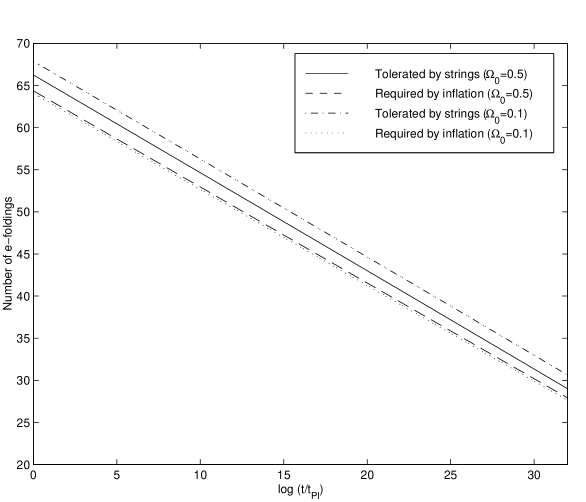
FIG. 1.: The maximum number of efoldings tolerated by a string network (formed at time $t$ shown in the horizontal axis) that is required to be inside the horizon at $t_{eq}$ and the number of efoldings in an open inflationary model such that the second inflationary period starts when the strings form and the present density is $0.5$ or $0.1$.

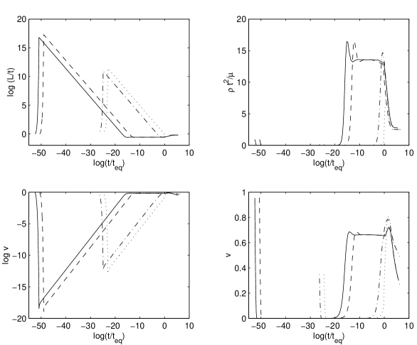
FIG. 2.: Evolution of GUT-scale string networks in open inflation models, for the following sets of initial conditions: $T_{r}=10^{15}\,GeV,\Omega_{0}=0.1$ (solid lines), $T_{r}=10^{15}\,GeV,\Omega_{0}=0.9$ (dashed), $T_{r}=10^{2}\,GeV,\Omega_{0}=0.1$ (dash-dotted) and $T_{r}=10^{2}\,GeV,\Omega_{0}=0.9$ (dotted).

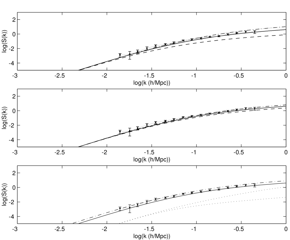
FIG. 3.: Comparing the CDM hybrid (strings plus inflation) power spectrum in open inflationary models, for several choices of $\Omega_{0}$, $h$ and $T_{r}$. In the top panel, the power spectra for $h=0.65$, $\alpha=0.5$ and $\Omega_{0}=0.7,\,0.5,\,0.3$ are shown (dot-dashed, solid and dashed lines respectively). In the middle pannel we plot the power spectra for $\Omega_{0}=0.5$, $\alpha=0.5$ and $h=0.75,\,0.65,\,0.55$ (dot-dashed, solid and dashed lines respectively). The lower pannel represents the power spectra for $\Omega_{0}=0.5$, $h=0.65$ and $\alpha=1,\,0.5,0.001$ (dot-dashed, solid and dotted lines respectively). The two dotted lines represent two different string networks in which strings come inside the horizon at the time $t\sim t_{\rm eq}$ and $t\sim 10^{-16}t_{\rm eq}$.

- [1] A.D. Linde, Particle Physics and Inflationary Cosmology (Harwood, Switzerland, 1990); K.A. Olive, Phys. Rep. 190, 307 (1990).
- [2] A. Vilenkin and E. P. S. Shellard, Cosmic Strings and other Topological Defects, (Cambrige University Press: Cambridge, 1994).
- [3] J.L. Tonry, Ann. N.Y. Acad. Sci. 688, 113 (1993).
- [4] M. Bucher, A.S. Goldhaber and N.G. Turok, Phys. Rev. D52, 3314 (1995);
- [5] A.D. Linde and A. Mezhlumian, Phys. Rev. D52, 6789 (1995).
- [6] J. Garcia-Bellido, J. Garriga & X. Montes, Phys. Rev. D57, 4669 (1998).
- [7] A. Vilenkin, Phys. Rev. D56, 3258 (1997).
- [8] C.J.A.P. Martins and E.P.S. Shellard, Phys. Rev. D53, 575 (1996); C.J.A.P. Martins and E.P.S. Shellard, Phys. Rev. D54, 2535 (1996).
- [9] P.P. Avelino, R.R. Caldwell and C.J.A.P. Martins, Phys. Rev. D56, 4568 (1997).
- [10] C.J.A.P. Martins, Quantitative String Evolution, Ph.D. Thesis, University of Cambridge (1997).
- [11] C.J.A.P. Martins, Astrophys. & Sp. Sci., in press (1998).
- [12] C.J.A.P. Martins and E.P.S. Shellard, Phys. Lett. B in press (1998); C.J.A.P. Martins and E.P.S. Shellard, Phys. Rev. D57 in press (see hep-ph/9804378).
- [13] C.J.A.P. Martins, Phys. Rev. D55, 5208 (1997).
- [14] A. Albrecht, R.A. Battye and J. Robinson, astro-ph/9711121 (1997).
- [15] E.F. Bunn, M. White, Astrophys. J., 480, 6 (1996); E.F. Bunn, A.R. Liddle, M.White, Phys. Rev. D54, R5917 (1996).
- [16] K. M. Gorski , B. Ratra, R. Stompor, N. Sugiyama and A. J. Banday, astro-ph/9608054 (1996)
- [17] D.H. Lyth, Phys. Rev. D31, 1792 (1985).
- [18] P.P. Avelino, E.P.S. Shellard, J.H.P. Wu, B. Allen, Phys. Rev. Lett. 81, 2008 (1998).
- [19] J.M. Bardeen, J.R. Bond, N.Kaiser, A.S. Szalay, Ap. J., 304, 15 (1986).
- [20] S.M. Carroll, W.H. Press, E.L. Turner, Ann. Rev. Astron. Astrophys., 30, 499 (1992).
- [21] J.A. Peacock and S.J. Dodds, Mon. Not. R. Astron. Soc. 267, 1020 (1994).
- [22] A. Albrecht and A. Stebbins, Phys. Rev. Lett. 68, 2121 (1992); A. Albrecht and A. Stebbins, Phys. Rev. Lett. 69, 2615 (1992).
- [23] C.J.A.P. Martins & E.P.S. Shellard, in preparation.
- [24] E.W. Kolb and M.S. Turner, Ap. J. 286, 702 (1984); K. Freese, M.S. Turner and D.N. Schramm, Phys. Rev. Lett. 51, 1625 (1983).
- [25] C. Contaldi, M. Hindmarsh & J. Magueijo, astro-ph/9809053 (1998).