The blue-bump of 3C 273

Abstract

We present optical and ultraviolet observations of 3C 273 covering the whole life of the IUE satellite. We analyze the variability properties of the light curves, and find that two variable components, written $\cal{B}$ and $\cal{R}$ respectively, must contribute to the blue-bump emission in this object.

The $\cal{B}$ component produces most of the variability in the ultraviolet domain. A maximum time scale of variability of about 2 yr identical at all wavelengths is found. If discrete events produce this component, the event rate is $\sim$3-30 yr^-1. Assuming an isotropic emission, each event must liberate about $10^{51}$ erg in the form of optical-to-ultraviolet radiation. The spectral properties of the $\cal{B}$ component suggest that reprocessing on a truncated disk, or partially-thick bremsstrahlung may be the emission mechanism. We find evidence of a lag of a few days between the light curves of the $\cal{B}$ component at optical and ultraviolet wavelengths. An irradiated geometrically-thick accretion disk model satisfies all the constraints presented here.

Neither the variability properties, nor the spectral properties of the $\cal{R}$ component can be accurately measured. This component varies on very long time scales, and may completely dominate the historical light curve of 3C 273 in the optical domain. Combining knowledge from other wavelengths, we obtain several indications that this component could reveal the “blazar” 3C 273. In particular, the light curve of this component is very similar to the hard X-ray light curve.

1 Introduction

Several components contribute to the multiwavelength continuum emission of active galactic nuclei (AGN). One of these components, which is called the “blue-bump”, contains the dominant fraction of the total emitted power in Seyfert 1 galaxies and (non-blazar) quasars. Understanding the emission process at its origin would therefore be a fundamental step towards the comprehension of the AGN phenomenon.

It is very easy to observe the blue-bump of the brightest Seyfert galaxies and quasars with optical telescopes. One of the first result of these observations is that these objects vary following complicated patterns (e.g., Press, 1978). This has been the motivation for important monitoring campaigns of the blue-bump emission of a few bright sources, among which the quasar 3C 273. The aim of these campaigns was to constrain the physics of the blue-bump using variability properties, either of the lines, or of the continuum. In this paper, we concentrate on the continuum emission, neglecting the emission line spectrum.

Very detailed models for the continuum emission of the blue-bump have been proposed, which can reproduce very correctly the optical-to-ultraviolet spectral energy distribution (and sometimes up to the soft X-ray, or even the hard X-ray, domain). They are often based on the presence of an accretion disk Shakura & Sunyaev (1973), and include the effect of Comptonization Czerny & Elvis (1987); Ross et al. (1992), the illumination by an X-ray source Collin-Souffrin (1991); Ross & Fabian (1993), or a corona Czerny & Elvis (1987); Haardt & Maraschi (1991); Haardt et al. (1994). More exotic models invoke optically thin emission Barvainis (1993), or supernova explosions Terlevich (1992). The reproduction of a particular spectrum is only the first requirement that a model has to fulfill. A further requirement is that the model can explain a series of simultaneous spectra. Such attempts to check whether the above-mentioned models satisfy to this second requirement have been made by Rokaki et al. (1992, 1993), Paltani & Walter (1996a) (hereafter PW96) and Loska & Czerny (1997). The final step would be to make sure that the complete dynamics of the spectra can be reproduced by the models, including variability time scales, spectral variations, and possible delays between blue-bump light curves.

In this paper we examine in detail the variability properties of the continuum emission of 3C 273. We have gathered nearly 20 years of observations with the International Ultraviolet Explorer (IUE) satellite and 10 years with an optical ground-based telescope. We perform temporal analyses to understand how 3C 273 varies, and we use the temporal and spectral knowledge gained in these analyses to constrain the physics of the emission at these wavelengths. Our approach differs from those used in the papers cited above (although we shall extend the work done in PW96) in that we focus on the time-series properties of the blue-bump light curves, without neglecting the spectral properties. Our goal is to achieve here one of the most complete analysis of the optical and ultraviolet emission ever done on an active galactic nucleus, and to express the most stringent possible constraints that are hidden in the huge amount of data collected on 3C 273.

2 The blue-bump continuum light curves

The data used in this paper are the IUE and optical observations (Geneva photometry only) described in Türler et al. (1998). Details about the data are to be found in this paper. For the IUE spectra, we used the IUESIPS data reduction, as the Final Archive was far from completion when we started the present analysis (Note however that the results are very similar with the new reduction). The IUE spectra identified as dubious in Türler et al. (1998) have been discarded . We corrected all the light curves for the effect of the reddening. We used the reddening law of Savage & Mathis (1979). The value of $E_{\mathrm{B-V}}$ has been set to 0.038, which is the value obtained in PW96. We finally obtained 191 IUE SWP spectra, 155 IUE LWP/LWR spectra, and 376 Geneva photometry optical observations.

We define 22 windows in the IUE spectra (7 for the SWP wavelength range and 15 in the LWP/LWR wavelength range) of width 50 Å, or 100 Å (at the beginning and the end of the LWP/LWR wavelength range, because of the large noise in these regions), carefully avoiding emission lines. It is unfortunately not possible to obtain optical light curves free of emission line contamination, as they have been obtained with broad-band photometry. However the contribution of the emission lines has been estimated to be at most of the order of 10 % Courvoisier et al. (1990). As Ly $\alpha$ variability is smaller than 10 % Ulrich et al. (1993), we do not expect that the optical light curves are significantly perturbed by the contamination. The average fluxes in these bins are plotted on Fig. 4.

Fig. 1a–d shows 4 of the ultraviolet light curves extracted from the IUE spectra. Fig. 1e–g shows three optical light curves, in the U, B and V filters respectively. One can see that all the ultraviolet and optical light curves are similar. It is however apparent to the eye that a large bump is present in the optical light curves (and in a less clear way in the 3 080–3 180 Å light curve), which is (almost) absent at 1 250–1 300 Å.

Figure 1: Ultraviolet and optical light curves from our database dereddened with $E_{\mathrm{B-V}}=0.038$. (a)–(d) IUE light curves. (e)–(g) Optical light curves from the Swiss telescope.

3 Rapid flares in 1988 and 1990

In 1988, Courvoisier et al. (1988) noted the occurence of several very rapid flares in the optical and near-infrared emission of 3C 273. Comparable, but somewhat weaker, events have occurred between May and June 1990. The details of the optical light curve are shown in Fig. 2. Unfortunately, the 1990 flares have been detected several weeks after the observations, and no special observation campaign has been performed.

On March 11, 1988, 3C 273 has been observed almost simultaneously (within a couple of hours) in the Geneva photometry and in near-infrared J, H, K, and L’ photometry Courvoisier et al. (1988). If one substracts the slowly varying continuum, one gets a power-law spectrum with a spectral index of 1.2 ($f_{\nu}\sim\nu^{-\alpha}$), as shown in Fig. 3, which is much redder than the mean optical spectral index, which is about 0.4. These flares have been discussed at length elsewhere Courvoisier et al. (1988); Robson et al. (1993), and will not be discussed further here. The observations marked by open circles in Fig. 2 present colour indices that depart significantly from the values obtained in adjacent observations, and hence are supposed to be obtained when 3C 273 was in a flare state. They are discarded in the rest of the present analysis.

Figure 2: Rapid flares in the V light curve of 3C 273. (a) in Spring 1988. (b) in Summer 1990 (see text). The circles represent data in which the contribution of the flares is important. These data have been discarded from the rest of the present analysis

Figure 3: Optical and near-infrared spectrum of the flare of March 11, 1988. The least-square linear regression has a slope $-1.2$ (solid line).

4 Variability properties of the blue-bump

4.1 Statistics of the light curves

Fig. 4a shows the mean ultraviolet-to-optical spectrum of 3C 273 as a function of the wavelength. It presents a small bump around $10^{14.9}$ Hz, which may be attributed to Fe ii and Balmer line and continuum emission. The rest of the spectrum is not very different from an unique power-law with an index $0.44$.

Figure 4: (a) Mean ultraviolet-to-optical continuum spectral energy distribution of 3C 273. The dashed line has a slope $-0.44$. (b) Standard deviation of the measurements in each band

On Fig. 4b, we can see the variability spectrum, i.e. the standard deviation as a function of the frequency. Contrarily to what is seen in the mean spectrum, an extrapolation of the ultraviolet variability clearly overestimates the variability in the V band. We do not believe that this feature can have an instrumental origin, as the transition between the ultraviolet and optical observations is smooth; this cannot be the result of a discrepancy in the absolute calibration between the two instruments, as it would produce a discontinuity. The important noise at the edges of the LWP/LWR wavelength range can be easily seen in Fig. 4.

4.2 Correlation analysis

We compare the light curves with each other using correlation analysis. In the case of astronomical discrete time series, two methods are generally used: the discrete correlation function (Edelson & Krolik, 1988, DCF) and the interpolated cross-correlation function (Gaskell & Peterson, 1987, ICCF). We use here the ICCF method, because it gives better results in case of the dense sampling available here White & Peterson (1994); Litchfield et al. (1995). We have however checked that the results obtained with both methods are qualitatively identical.

Fig. 5 shows the correlations between the 1 250-1 300 Å light curve and the seven light curves from Fig. 1 as a function of the lag $\tau$. Two features emerge from these correlations. First, a peak close to $\tau=0$. Its amplitude decreases with the wavelength, but is still large ($\sim$ 0.75) in the correlation with the optical V light curve. The width of the peak does not show any evidence of broadening when the wavelength increases. It means that an important fraction of the emission in the long-wavelength light curves varies in unison with the shortest-wavelength light curve. One has however the impression that the central peak is shifted towards larger values of $\tau$, and the more so as the wavelength of the second light curve increases. This is an indication of a possible (short) lag between the light curves. This is analyzed in more details in Sect. 6.

The second feature is a hump between 0 and 2 yr. Correlation analysis must be taken with caution when dealing with discrete, unevenly-sampled time series, as features without any physical reality can be generated by sampling effects. We have first attributed this second feature to this phenomenon. However, its amplitude increases monotonically with the wavelength, a behaviour that cannot be due to the sampling. We shall discuss further this feature in Sect. 7.2.

Figure 5: Correlations between the IUE 1 250-1 300 Å light curve and other IUE and optical light curves (successive solid lines). The effect of increasing the wavelength of the second light curve is shown for the peak at 0 lag (1), and for the hump (2)

4.3 Variability time scales

We investigate the variability time scales of the blue-bump of 3C 273 using structure function analysis. The structure function approach has been introduced in astronomy by Simonetti et al. (1985). The first-order structure function of a light curve (referred to as “SF” hereafter) is formally equivalent to its autocovariance. It however highlights some important properties of the light curve in a much clearer way. The SF of a time series $x(t)$ is a function of a time lag “$\tau$”, and is defined by:

$$\mathrm{SF}_{x(t)}(\tau)=\left<\left(x(t+\tau)-x(t)\right)^{2}\right>$$ (1)

where $<\!z(t,\ldots)\!>$ is the average of $z$ over $t$. We have calculated SFs for the 29 optical and ultraviolet continuum light curves. The result is presented on Fig. 6 for seven of them.

Figure 6: a–g Structure functions of 7 ultraviolet and optical light curves. The solid line is the best fit with the function given by Eq. (2).

Let us assume that a time series $x(t)$ has a non-zero Fourier power-spectrum only at frequencies larger than $f_{\mathrm{min}}$. Below $\tau_{\mathrm{max}}=(f_{\mathrm{min}})^{-1}$, the larger $\tau$, the larger the part of the power-spectrum that can make the time series vary; thus the SF increases with $\tau$. Above $\tau_{\mathrm{max}}$, all the power of the Fourier spectrum can be used to make $x(t)$ vary, and the SF remains constant at a value equal to twice the variance of $x(t)$. One can convince oneself of this result by noting that $x(t)$ and $x(t+\tau_{0})$ with $\tau_{0}>\tau_{\mathrm{max}}$ are completely uncorrelated, and therefore their variances add up. Similarly, if one observes $y(t)=x(t)+\varepsilon(t)$, where $\varepsilon(t)$ is a white noise representing the measurement uncertainties, then a constant is added to the SF equal to twice the variance of $\varepsilon(t)$. This constant comes from the fact that $\varepsilon(t)$ and $\varepsilon(t+\tau_{0})$ are completely uncorrelated, $\forall\tau_{0}\neq 0$.

In Fig. 6a, we observe that a plateau is reached around $\tau\simeq 0.5$ years. However, in the SFs at longer wavelengths (especially in the optical domain; cf. Figs 6d–f), the SFs still increase for $\tau\simeq 10$ years. We have checked that this was not due to the difference in time spans between the ultraviolet and optical light curves by comparing the SF of a truncated ultraviolet light curve with that of the total light curve. Both SFs are indeed undistinguishable. To extract the quantitative information contained in the SFs, one may wish to fit them with some analytical function, and, if possible, the same for all the light curves. We have found one function that fits rather well all SFs, and whose parameters may have a physical interpretation. This function is given by:

$$f(\tau)=2\cdot p_{0}^{2}+\left\{\begin{array}[]{ll}p_{2}\cdot(\frac{\tau}{p_{1}})^{p_{3}},&\mathrm{if\leavevmode\nobreak\ }\tau<p_{1}\\ p_{2},&\mathrm{if\leavevmode\nobreak\ }\tau\geq p_{1}\\ \end{array}\right\}+p_{4}\cdot\tau^{2}$$ (2)

This function contains three separate terms:

• the measurement uncertainty, given by $p_{0}$, whose contribution to the SF is twice its square.

• the $\cal{B}$ term (in anticipation to Sect. 5), whose SF is a power-law that increases with an index $p_{3}$ until a plateau is found at $\tau=p_{1}$. After the plateau, this term remains constant at a value $p_{2}$.

• The $\cal{R}$ term (again, see Sect. 5), whose SF is a power-law with an index 2, which is the maximum index that can be exhibited by a SF. It describes a long-term variation.

The justification of Eq. (2) is that the SF is linear, i.e. $\mathrm{SF}_{x(t)+y(t)}(\tau)=\mathrm{SF}_{x(t)}(\tau)+\mathrm{SF}_{y(t)}(\tau)$, if $x(t)$ and $y(t)$ are completely uncorrelated for all $\tau$. The result of the fits to seven SFs are shown on Fig. 6. The values of the 5 parameters as a function of the wavelengths are displayed in Fig. 7.

$p_{0}$ (Fig. 7a) is an experimental determination of the uncertainty. Comparing this parameter to the mean spectrum, one sees that the relative uncertainty reached is between 2.7 and 4.6 % with IUE observations, and between 1.2 and 2.6 % with the optical observations.

$p_{1}$ (Fig. 7b), the end of the short-term variation, does not show evidence of variation throughout the 29 light curves, with a mean of 0.46 yr, and a very small dispersion of 0.054 yr. Note however that, to achieve this result, the value of $p_{1}$ has been constrained to be smaller than 1 yr in the 2 “reddest” IUE light curves (otherwise, $p_{1}$ becomes larger than 10 yr). We adopted this procedure, only because unconstrained fits to the optical SFs give again values very close to 0.46 yr. It therefore appears to us that the same plateau is identified in all the ultraviolet and optical lightcurves, the more so as the samplings in the optical and ultraviolet domains are completely different.

Figure 7: Parameters derived from the SFs. (a) $p_{0}$, the measurement uncertainty. (b) $p_{1}$, the location of the plateau. (c) $p_{2}/p_{2}[V]$, the amplitude of the $\cal{B}$ term relatively to its amplitude in the V filter. (d) $p_{3}$, the slope of the increasing part of the $\cal{B}$ term. (e) $p_{4}/p_{4}[V]$, the amplitude of the $\cal{R}$ term relatively to the its amplitude in the V filter.

$p_{2}$ (Fig. 7c) is the amplitude of the $\cal{B}$ term of the SFs. It decreases slowly in the ultraviolet domain, but much more rapidly in the visible domain; this is comparable to the variability spectrum (Fig. 4b).

$p_{3}$ (Fig. 7d) is the slope of the $\cal{B}$ term of the SFs. The slope of the SF is related to that of the Fourier power spectrum: The larger the slope of the SF, the smaller that of the Fourier power spectrum. $p_{3}$ decreases with wavelength, mostly in the optical domain. This indicates that variability on short time scale is comparatively more important in the optical domain than in the ultraviolet domain. Caution must however be taken with this direct interpretation. The shape of the $\cal{R}$ term has been set arbitrarily, and the value of $p_{3}$ may be affected by this choice.

$p_{4}$ (Fig. 7e) determines crudely the amplitude of a longer-term variation (whose real SF is unknown). This $\cal{R}$ term is clearly needed in the optical domain, but is much less evident in the ultraviolet domain, and its amplitude at these wavelengths is mostly defined by a handful of values at the end of the ultraviolet SFs, and thus not reliable. One sees however that its amplitude increases dramatically above 2 800 Å, and joins with little discontinuity the amplitude measured in the U band. This shows that the $\cal{R}$ term probably exists in the ultraviolet domain, although its intensity is difficult to estimate.

5 The two components of the blue-bump of 3C 273

Eye inspection of the light curves, and the results from Sect. 4.3 give the impression that there are really two differently varying components in 3C 273. We propose here a method to decompose the light curves into these two tentative components.

5.1 Decomposition method

PW96 have observed that the ultraviolet fluxes at two different wavelengths are very well connected by an affine relationship (cf. Fig. 1 and the discussion in Sect. 2.2 & 2.3 in PW96). They therefore claimed that the blue-bump light curves could be the sum of two components:

$$f(\nu,t)=V_{\nu}\cdot\varphi(t)+S_{\nu},$$ (3)

where $V_{\nu}\cdot\varphi(t)$ is a variable component and $S_{\nu}$ is a stable component. $\varphi(t)$ is a function that determines the complete temporal behaviour of the ultraviolet emission of the source. It is unknown, but it can be approximated by a “reference flux”, the flux in a window located at the “blue” end of the IUE spectra (around 1 250 Å). Using this reference flux, one can derive the exact spectral shape of $V_{\nu}$ (but not its normalization), and a set of possible $S_{\nu}[x]$ distribution, $0\!\leq\!x\!\leq\!1$, $x\!=\!0$ maximizing the contribution of $V_{\nu}\cdot\varphi(t)$ at the frequency of the reference flux, and $x\!=\!1$ minimizing it.

Sect. 4.3 shows that Eq. (3) cannot explain all the light curves. We test the possibility that what has been called “stable component” in PW96 is actually variable. Eq. (3) could be modified in the following way:

$$f(\nu,t)=V_{\nu}\cdot\varphi(t)+S_{\nu}(t),$$ (4)

Provided that $|S_{\nu}(t_{1})-S_{\nu}(t_{2})|\ll V_{\nu}\cdot|\varphi(t_{1})-\varphi(t_{2})|,\forall t_{1},t_{2}$, Eq. (3) is a sufficient approximation of Eq. (4). This is why it could be applied in PW96. With the increase of the time span of the observations, and the addition of optical measurements, this condition is not satisfied anymore. Hereafter we shall write “$\cal{B}$”, and “$\cal{R}$” respectively the components $V_{\nu}\cdot\varphi(t)$, and $S_{\nu}(t)$ in Eq. (4). Their contributions to the SFs will be the $\cal{B}$ and $\cal{R}$ terms respectively. We try to solve Eq. (4) by fitting the light curves with the sum of the $\cal{B}$ and the $\cal{R}$ components. The $\cal{B}$ component is given by the 1 250–1 300 Å light curve and normalized by an unknown parameter. We have a priori no information on the $\cal{R}$-component light curve; we therefore define its light curve with 8 parameters, which are the values of a cubic-spline function at abcissae 1984, 1986,…, 1998 yr. The result of these fits are shown for seven light curves in Fig. 8. Note that the fits cannot be perfect in the optical domain, because the value of $\varphi(t)$ must be interpolated from the IUE observations. The general agreement is however very good.

Figure 8: a–g Two-component fits to 7 light curves with the ${\cal R}^{\mathrm{min}}$ assumption. h–n idem with the ${\cal R}^{\mathrm{max}}$ assumption. The thick solid line is the sum of the two components, the $\cal{B}$ component (dashed line), and the $\cal{R}$ component (thin solid line).

As in PW96, the decomposition is not unique. Indeed the $\cal{R}$ component may contribute at 1 250 Å also. The problem is actually worse than in PW96, as it is not only a constant that is unknown, but a whole light curve. We fix the maximum $\cal{R}$ component by assuming that it goes smoothly through the successive minima of the 1 250-1 300 Å light curve (those around $t=1987.5,\leavevmode\nobreak\ 1990,\leavevmode\nobreak\ 1992,\leavevmode\nobreak\ 1993,\leavevmode\nobreak\ 1993.5,1994,\leavevmode\nobreak\ \mathrm{and}\leavevmode\nobreak\ 1995$). We shall call “the ${\cal R}^{\mathrm{min}}$ (resp. ${\cal R}^{\mathrm{max}}$) assumption” the result of the decompositions with the assumption of a negligible (resp. maximal) $\cal{R}$ component at 1 250-1 300 Å.

5.2 The $\cal{B}$ component

The shape of the $\cal{B}$ component is shown on Fig. 9. As in PW96, its normalization, but not its spectral shape, depends on the assumption made on the $\cal{R}$ component. There is a clear curvature in the ultraviolet-to-optical spectrum, and it is clearly not possible to fit the entire spectrum with a single power-law. The absence of discontinuity shows that this curvature cannot be due to an instrumental problem. A fit with two power-laws gives an index of $-0.16$ at wavelengths shorter than 2 600 Å, and about $-1$ at wavelengths longer than 2 600 Å ($f_{\nu}\sim\nu^{-\alpha}$). Note that the curvature in the $\cal{B}$ spectral energy distribution has already been observed for a subset of the data covering the years before 1991, and where the $\cal{R}$ component was considered constant Paltani & Walter (1996b), and it is therefore not an artifact produced by the introduction of a varying $\cal{R}$ component.

5.3 The $\cal{R}$ component

We can see in Fig. 8 that the smoothed light curves of both the ${\cal R}^{\mathrm{min}}$ and ${\cal R}^{\mathrm{max}}$ components are very similar at all wavelengths: they show a minimum around 1989–1990 and a maximum around 1993-1994. It is important to remark that no a priori assumption on the light curve has been made in the ${\cal R}^{\mathrm{min}}$ case. The similarity of the $\cal{R}$ component at all the different frequencies is an argument in favour of the reality of the decomposition.

Figure 9: Spectral energy distribution of the $\cal{B}$ component normalized to its amplitude at 1 250 Å.

Figure 10: Spectral energy distribution of the $\cal{R}$ component. (a) ${\cal R}^{\mathrm{min}}$. (b) ${\cal R}^{\mathrm{max}}$. In each panel, upper curve: $t=1993.0$ (maximum flux); lower curve: $t=1989.0$ (minimum flux)

The ${\cal R}^{\mathrm{min}}$ and ${\cal R}^{\mathrm{max}}$ spectral energy distributions at $t=1993.0$ and $t=1989.0$ (the extrema) are plotted on Fig. 10. There is still a strong flux below (in frequency) the Balmer edge, which can be explained neither by emission lines, nor Balmer, and Paschen continua, although they can modify slightly the shape of the $\cal{R}$ component (in particular, the small bump around $10^{14.9}$ Hz can be explained by Balmer continuum and line emissions). The ${\cal R}^{\mathrm{min}}$ component deviates strongly from a unique power-law, while the ${\cal R}^{\mathrm{max}}$ component is compatible with a single power-law of index about $0.7$.

6 Delay between the light curves

Fig. 5 already indicates that the correlation peak close to $\tau=0$ has an amplitude that decreases and a centroid that moves slightly towards larger values of $\tau$ as the wavelength of the second light curve increases. Fig. 11 emphasizes this effect with a closer look at the central peak of the same correlations for the complete light curves, and for the $\cal{B}$ components obtained with the ${\cal R}^{\mathrm{min}}$ and ${\cal R}^{\mathrm{max}}$ assumptions respectively. This is an evidence for a delay between the different light curves.

Figure 11: Correlations between the IUE 1 250-1 300 Å light curve and 7 IUE and optical light curves (the thicker the line, the larger the wavelength of the second light curve). (a) Total light curves. (b) $\cal{B}$ with the ${\cal R}^{\mathrm{min}}$ assumption. (c) $\cal{B}$ with the ${\cal R}^{\mathrm{max}}$ assumption

Table 1: Results of the “$\tau$” test. “Probability” is the probability that the test performed on uncorrelated parent populations gives a value of $\tau$ smaller or equal to the measured one

Light curves	Total			$\cal{B}$ with ${\cal R}^{\mathrm{min}}$			$\cal{B}$ with ${\cal R}^{\mathrm{max}}$
	$t_{2}$ (days)	$\tau$	Probability	$t_{2}$ (days)	$\tau$	Probability	$t_{2}$ (days)	$\tau$	Probability
All	$13.8$	$-0.79$	$0^{*}$	$\phantom{0}4.2$	$-0.66$	$0^{*}$	$\phantom{0}4.4$	$-0.66$	$0^{*}$
SWP		$-0.90$	$1.0\,10^{-5}$		$-0.33$	$9.4\,10^{-2}$		$-0.33$	$9.4\,10^{-2}$
LWP/LWR		$-0.44$	$2.5\,10^{-6}$		$-0.56$	$3.0\,10^{-9}$		$-0.56$	$3.0\,10^{-9}$
Optical		$-0.71$	$7.4\,10^{-4}$		$-1.00$	$4.8\,10^{-7}$		$-0.90$	$1.0\,10^{-5}$

^∗These probabilities are formally smaller than $10^{-40}$

In view of Fig. 11, we would like to establish the statistical significance of the delay, and, assuming that it is real, estimate its amplitude. Note that the decomposition is still valid in spite of the delay, because the value of the correlation at $\tau=0$ is very close to its maximum. The lags have been estimated using cross-correlation analysis (as in Sect. 4.2). More sophisticated methods have been tried, but they gave less reliable results. The $\chi^{2}$ method of Press et al. (1992a) is not appropriate, because the covariance matrix is dominated by measurement uncertainties, and thus badly known, at very short lags, where we expect to find the delay. The “dispersion spectrum” method of Pelt et al. (1994) suffers from a similar problem, namely that, because of the short lags investigated, most of the pairs of observations used in the calculation of the “dispersion spectrum” are separated by too long a delay. We note however that the qualitative results obtained with these two methods are compatible with those obtained with the ICCF.

We define a procedure to estimate the delay between two light curves using the ICCF method: First we calculate the $29\times 29$ ICCFs between all the pairs of light curves for $-0.1\!\leq\!\tau\!\leq\!+0.1$ yr; then we fitted a 2nd-degree polynomial to the ICCF, whose abscissa of the maximum defines the delay. We did this for the observed light curves, the $\cal{B}$ component with the ${\cal R}^{\mathrm{min}}$ assumption, and the $\cal{B}$ component with the ${\cal R}^{\mathrm{max}}$ assumption. We then calculate the average delay $\tilde{\Delta}_{i}$ between the first and the $i^{\mathrm{th}}$ light curve (1 250–1 300 Å) with the relationship:

$$\tilde{\Delta}_{i}=\frac{1}{n}\leavevmode\nobreak\ \sum_{j=1}^{n}\leavevmode\nobreak\ \Delta_{1,j}+\Delta_{j,i},$$ (5)

where $n=29$ is the number of light curves, and $\Delta_{k,\ell}$ is the delay between the $k^{\mathrm{th}}$ and the $\ell^{\mathrm{th}}$ light curves. A positive delay means that the first light curve precedes the seconds one. This average has the purpose to decrease the effect of the uncertainties on the lags. The $\tilde{\Delta}_{i}$ delay curves are shown in Fig. 12, together with the dispersion of the individual delays used in the calculation of $\tilde{\Delta}_{i}$.

Figure 12: Delay with respect to the first light curve. The points are the delays averaged on the 29 measurements, and the dashed lines show their 3$\sigma$ dispersion. The thick line is the fitted delay. (a) Total light curves. (b) $\cal{B}$ with the ${\cal R}^{\mathrm{min}}$ assumption. (c) $\cal{B}$ with the ${\cal R}^{\mathrm{max}}$ assumption

The delays can be approximated by the function: $\tilde{\Delta}_{i}\simeq t_{2}\cdot\log_{2}(\lambda_{i}/1\,275\mbox{\leavevmode\nobreak\ \AA})$. The parameter $t_{2}$ gives the delay observed between two light curves at wavelengths $\lambda_{0}$ and $2\cdot\lambda_{0}$ respectively. Their values in the three cases are reported in Table 1. No difference can be observed between the ${\cal R}^{\mathrm{min}}$ and ${\cal R}^{\mathrm{max}}$ decomposition, with a $t_{2}$ of about 4 days, but the $t_{2}$ obtained without decomposition is 3 times larger. This could be due to a contamination by the $\cal{R}$ component (see Sect. 7.2).

The global significance of the existence of a delay can be tested by a modified Kendall’s $\tau$ test (e.g. Press et al., 1992b). The original test (and the version used below) has the very interesting property to be completely non-parametric. Assuming a set of data $(x_{i};y_{i}),\leavevmode\nobreak\ i=1,\ldots,n$, the $\tau$ test actually measures the excess of “concordant” (or alternatively “discordant”) pairs of data taking into account all the possible pairs, a pair of data $[(x_{i};y_{i});(x_{j};y_{j})]$ being called “concordant” (respectively “discordant”) if either ($x_{i}\!>\!x_{j}$ and $y_{i}\!>\!y_{j}$), or ($x_{i}\!<\!x_{j}$ and $y_{i}\!<\!y_{j}$) (respectively, if either ($x_{i}\!<\!x_{j}$ and $y_{i}\!>\!y_{j}$), or ($x_{i}\!>\!x_{j}$ and $y_{i}\!<\!y_{j}$)). We cannot use directly this scheme, as a delay is not defined for one wavelength, but only for a couple of wavelengths. We therefore replace the condition $y_{i}\!>\!y_{j}$ (for instance) by the condition $\Delta_{i,j}\!>\!0$. Kendall’s $\tau$ can then be estimated using Eq. (14.6.8) of Press et al. (1992b). The probability to obtain a given value for $\tau$ from uncorrelated parent populations (which means in this case that their lags are random) can be calculated from simple combinatorics arguments.

Table 1 gives the correlation coefficients and the probability that the test performed on two uncorrelated populations gives a value of $\tau$ smaller or equal to the measured one. The minus sign indicates that the long-wavelength light curves follow the short-wavelength ones, compatible with Fig. 12. If one uses the 29 light curves, it is absolutely impossible that the correlation coefficients are obtained by chance. However it is possible that the correlation is due to the sampling. To exclude this possibility, we have applied the $\tau$ test to light curves that have exactly the same sampling. Here also, the probabilities that the correlation coefficients are obtained by chance are completely negligible. As the tests are independent, the probabilities to obtain these correlation coefficients are smaller than $10^{-15}$ both for the complete light curves and those of the $\cal{B}$ components. Thus we conclude that the existence of a lag is firmly established.

7 Discussion

7.1 Is the decomposition physical?

The similarity of the central peaks in all the correlations and the important differences in the structure functions offer a very compelling argument in favour of the physical existence of two separate $\cal{B}$ and $\cal{R}$ components. They imply that the long term variability is not the result of “dilution” of the light curve seen at short wavelength by a larger emission size or a longer cooling time scale, as the central peak would have appeared more and more smeared when the wavelength increases. The absence of smearing is confirmed by the structure function analysis, which shows that the $p_{1}$ parameter (see Eq. (2)) is constant. The fact that the “birth” of the $\cal{R}$ component can be seen in the rapid increase of $p_{4}$ around 2 800 Å is a strong argument against an instrumental origin of this component.

The light curves of the $\cal{R}$ components were completely free parameters in the fits of Sect. 5.1. In spite of this, the light curves of the ${\cal R}^{\mathrm{min}}$ and ${\cal R}^{\mathrm{max}}$ components are all very similar, and the resulting spectrum (Fig. 10) is smooth and quasi-monotonical. The near-infrared light curves Türler et al. (1998) are similar to the one of the $\cal{R}$ component, while no variation in the form of the $\cal{B}$ component is detectable at these wavelengths. Because of its spectral shape, the near-infrared emission of 3C 273 is usually attributed to thermal emission from hot dust Barvainis (1987). This component has a negligible contribution in the optical domain, because dust is destroyed at temperature above $\sim$1 500 K, and should also be constant on time scales of the order of the year, as the size of the emitting region is about 10 pc Barvainis (1987). Thus we conclude that another variable component contributes to the near-infrared emission of 3C 273, and that it is very probably the $\cal{R}$ component, owing to the similarity of the light curves.

Taking these points into account, we consider that the mathematical decomposition of Eq. (4) succeeds in isolating two independent physical components present in both the ultraviolet and optical light curves of 3C 273.

7.2 The lag and the hump in the correlations

Figure 13: Correlation between the $\cal{B}$ component at 1 250-1 300 Å and respectively the optical V light curve (solid line) and the $\cal{B}$ component in the optical V band (dashed line).

We observed the presence of a hump between 0 and 2 yr in the correlations shown in Fig. 5. On Fig. 13, we have plotted the correlation between the $\cal{B}$ component with the ${\cal R}^{\mathrm{max}}$ assumption at 1 250-1 300 Å and the optical V light curve (solid line). Again, a similar structure is found. If one calculates the correlation between the $\cal{B}$ component at 1 250-1 300 Å and the $\cal{B}$ component in the optical V light curve (dashed line), the hump is strongly suppressed. We conclude that the hump appears whenever a light curve containing the $\cal{B}$ component is correlated to another one containing the $\cal{R}$ component. A much longer monitoring would be necessary to determine whether this feature is real, or due to some soincidence in the light curves. If its reality is confirmed, it would have important consequences on the interpretations of the $\cal{B}$ and $\cal{R}$ components, as it would suggest a physical connection between the two components.

The hump may affect the shape the central peak, and hence its centroid. This cannot fully explain the lags that we have found, as we also observe a lag when the $\cal{R}$ component is removed. It can however explain why a longer lag is observed when the $\cal{R}$ component is not removed. The value of the lag is unchanged, whether we choose the ${\cal R}^{\mathrm{min}}$ or the ${\cal R}^{\mathrm{max}}$ assumption. It means that the influence of the $\cal{R}$ component is negligible even with the ${\cal R}^{\mathrm{min}}$ assumption. We therefore conclude that the lag is a property of the $\cal{B}$ component, and that the correct amplitude of the lag is $t_{2}\simeq 4$ days.

It is the second time that a lag between the different light curves of the blue-bump of an AGN is found. The first object is NGC 7469, where a lag has been detected both within the IUE SWP wavelength range Wanders et al. (1997), and between IUE and optical light curves Collier et al. (1998). The value of $t_{2}$ in NGC 7469 is 0.6 day. The average ultraviolet luminosity of NGC 7469 at 1 300Å is about $1.5\,10^{27}$ erg s^-1 Hz^-1, 1000 times less luminous than 3C 273 ($1.25\,10^{30}$ erg s^-1 Hz^-1). It suggests that the lag may increase with $L_{1250\leavevmode\nobreak\ \mbox{\scriptsize\AA}}^{1/3}$.

7.3 The nature of the $\cal{B}$ component

7.3.1 Time-series properties

Since the broadness of the Fourier transform of AGN light curves has been demonstrated (to our knowledge by Kunkel (1967)), many works have stated that the Fourier power-spectra of AGN light curves follow a power-law. From the $p_{3}$ parameter we can estimate that the index of the power-law would be about $-2.5$, which is, for instance, too steep to be due to a random-walk process. It must be realized however that almost any poorly-known broad Fourier power-spectra will appear power-law-shaped. Thus we do not want to discuss more the power-law index deduced from the $p_{3}$ parameter.

The $p_{1}$ parameter is the signature that there exists a frequency below which the Fourier power spectrum becomes negligible. Comparison with SFs of simulated light curves shows that this frequency is about 0.65 yr^-1. This means that the system that emits the $\cal{B}$ component has no “memory” of the state that it had 2 yr before. It is not obvious to find a physical continuous system that explains this low-frequency cut-off. However, the discrete-event models Paltani & Courvoisier (1997) naturally incorporate such a feature. This is discussed in Sect. 7.3.2.

The Fourier power-spectrum of a light curve has a high-frequency limit due to the size of the source (in the direction perpendicular to the observer). From the V light curve (which has the smallest uncertainties), a lower limit on the high-frequency limit can be put to $\sim$(10 day)^-1. Crossed at the speed of light, it corresponds to about 100 Schwarzschild radii (R_S) of a black hole with a mass $10^{9}$ M_⊙. This is only the limit size parallel to the observer’s direction. In particular, as 3C 273’s jet is seen with an angle of about $10^{\circ}$ (as deduced from the presence of superluminal motions), an accretion disk perpendicular to the jet could be much larger.

7.3.2 A discrete-event model interpretation of the variability

We explore the possibility that the variability of the $\cal{B}$ component is due to events occurring at random epochs. The main reason to make this assumption is that the $\cal{B}$ component would naturally exhibit a maximum variability time scale, as soon as the events have a finite life time. It can indeed be shown that the SF of a superimposition of an arbitrary number of similar events is proportional to the SF restricted to one single event Paltani (1996). Thus, the SF of the total light curve will be constant for all $\tau$ larger than the event life time.

Figure 14: Light curve and parameters of the events used in Sect. 7.3.2

We want to check whether all the observed variability properties of the $\cal{B}$ component can be reproduced. Let us use a very simple event shape, namely a triangular one, shown in Fig. 14. Its parameters are the time of birth of the event, $T_{0}$ (expressed in yr; this is the only parameter allowed to be different for each event), the event amplitude, $H$ (expressed in erg s^-1 Hz^-1), and the time needed to reach the maximum flux, $\mu$ (expressed in yr). A further parameter is the average event rate $\overline{N}$ (expressed in number of events per yr). The light curve properties that have to be matched are: the mean flux, the observed variance, and the location of the plateau in the SF. In principle the shape of the increasing part of the SF must also be matched, but the SF is not very sensitive to changes in the event shape, and practically any reasonable event shape fits the SF. The location of the plateau is only a function of $\mu$, and it corresponds to the one found in the SF of the $\cal{B}$ component if $\mu\simeq 0.4$ yr (this means that the total duration of an event is $0.8$ yr). From Eqs (11) and (B2) of Paltani & Courvoisier (1997), we find the following relationships for the mean luminosity and its variance (assuming that the ${\cal R}^{\mathrm{max}}$ assumption is correct):

$$\left\{\leavevmode\nobreak\ \begin{array}[]{llll}\overline{L_{1250/(1+z)\leavevmode\nobreak\ \mbox{\scriptsize\AA}}}&=&\overline{N}\cdot H\cdot\mu&=\\ &=&3.32\,10^{29}\mathrm{\leavevmode\nobreak\ erg\leavevmode\nobreak\ s}^{-1}\mathrm{\leavevmode\nobreak\ Hz}^{-1}\\[5.69054pt] {\mathrm{Var}}(L_{1250/(1+z)\leavevmode\nobreak\ \mbox{\scriptsize\AA}})&=&\overline{N}\cdot H^{2}\cdot\frac{2}{3}\mu&=\\ &=&5.99\,10^{58}\mathrm{\leavevmode\nobreak\ (erg\leavevmode\nobreak\ s}^{-1}\mathrm{\leavevmode\nobreak\ Hz}^{-1})^{2}\\ \end{array}\right.$$ (6)

where $z=0.158$ is the redshift. The mean luminosity and the variance of the $\cal{B}$ component are calculated using a Hubble constant $H_{0}=60$ km s^-1 Mpc^-1, and a deceleration parameter $q_{0}=0.5$. We can solve Eq. (6), which gives:

$$\left\{\leavevmode\nobreak\ \begin{array}[]{llrl}\overline{N}&=&3.07&\mathrm{\leavevmode\nobreak\ events/yr}\\ H&=&2.7\,10^{29}&\mathrm{\leavevmode\nobreak\ erg\leavevmode\nobreak\ s}^{-1}\mathrm{\leavevmode\nobreak\ Hz}^{-1}\\ \mu&=&0.4&\mathrm{\leavevmode\nobreak\ yr}\\ \end{array}\right.$$ (7)

Using ${\cal R}^{\mathrm{min}}$, the event luminosity is slightly smaller, and 30 events per year are required. Assuming that the event shape is the same at all wavelengths, Fig. 9 allows us to calculate $H$ as a function of the frequency. We deduce that the total event energy between 1 200 and 6 000 Å (observed wavelengths) is $3\,10^{51}$ erg, if the emission is isotropic. We can therefore rule out models where the events are supernova explosions Terlevich (1992) for energetic reason, as it is 100 times larger than the luminous energy of a supernova. If the $\cal{B}$ component is responsible for the soft-excess component, as suggested by Walter & Fink (1993), and extends up to 100 eV, the total event energy becomes of the order of $10^{52}$ erg. We note that using different event shapes would change the details of the figures, but not their orders of magnitude.

Courvoisier et al. (1996) have proposed that the luminosity originates from the kinetic energy of colliding stars. Fixing the black hole mass to $10^{9}$ M_⊙, it is possible to reproduce satisfactorily the variability properties of the $\cal{B}$ component, if the central stellar density is $10^{12}$ stars pc^-3, and if the core radius is 100 R_S ($\equiv 10^{-2}$ pc, or 10 light-days) in the ${\cal R}^{\mathrm{min}}$ case, and 40 R_S in the ${\cal R}^{\mathrm{max}}$ case. This cluster would contain about $10^{6}$ stars inside its core radius.

The magnetic blobs introduced by Galeev et al. (1979) and used by Haardt et al. (1994) are another kind of event candidates. To store $10^{52}$ erg in the form of magnetic energy with a field of $10^{5}$ G requires a volume of the order of $10^{40}$ cm³, i.e. a cube with a side of $10^{13}$ cm (0.1 R_S). To check the plausibility of these values would require a detailed physical treatment of the phenomenon, which is out of the scope of this work.

7.3.3 Synchrotron radiation model of the $\cal{B}$ component

Synchrotron emission has been considered as a candidate for the blue-bump emission. To obtain a ultraviolet spectral energy distribution comparable to the one of the $\cal{B}$ component, a synchrotron emitting medium requires a very flat electron energy distribution, with an index not smaller than $\sim-1.3$. The optical part of the $\cal{B}$ component requires then that the medium becomes self-absorbed around $\nu=10^{15}$ Hz. Using the formulae of Rybicki & Lightman (1979), we find that, if the electron energy distribution is given by $N(\gamma)\propto\gamma^{-1.2}$, and if $B=1$ G, it requires the size of the emitting medium to be of the order of $10^{8}$ cm, and an electron density of the order of $10^{23}$ cm^-3. The size depends little on the magnetic field, the electron energy distribution index, and even Doppler boosting. The required electron density is still $\sim 10^{21}$ cm^-3 if the magnetic field is fixed to 1 T. The Thompson opacity of this medium is extremely high ($>10^{6}$), which means that inverse Compton cooling must strongly dominate synchrotron radiation, and thus make the ultraviolet emission vanish, which rules out synchrotron radiation as the explanation of the blue-bump of 3C 273.

7.3.4 Bremsstrahlung radiation model of the $\cal{B}$ component

Optically-thin thermal bremsstrahlung emission already had some difficulty in fitting the $V_{\nu}$ component in 3C 273 (PW96), as the emission from such a mechanism has a spectral index of $\sim$0.2 when $\mathrm{h}\nu\!\ll\!\mathrm{k_{B}}T$ (e.g., Gronenschild & Mewe, 1978; Barvainis, 1993), where h is Planck’s constant, $\mathrm{k_{B}}$ Boltzmann’s constant and $T$ the temperature of the optically thin medium. It follows from this property that a flux distribution entirely due to optically thin emission cannot have parts of its spectrum with negative spectral index, whatever the temperature distribution of the emitting medium. The spectral index of the $\cal{B}$ component in the optical domain is clearly negative, which rules out the possibility of this emission mechanism in this object.

On the other hand, thermal bremsstrahlung emission can be partially, or even fully, optically thick. In that case, the thicker the emitting medium, the closer the emitted spectrum to the one of a blackbody. We calculated the spectrum of thermal bremsstrahlung emission for a plane-parallel geometry using the formulae of Rybicki & Lightman (1979). The $\cal{B}$ distribution can be very well fitted with such a model. If one imposes a temperature of $2.73\,10^{6}$ K (which is the temperature obtained by Walter et al. (1994) with a fit on ultraviolet and soft X-ray simultaneous observations) in the whole emitting medium, the electron density is $9\,10^{13}$ cm^-3, if the geometrical depth is $10^{13}$ cm. The emitting medium becomes optically thick ($\tau_{\nu}=1$) below $9.5\,10^{14}$ Hz ($\simeq$ 3150 Å).

Nayakshin & Melia (1997) have developed an interesting model where bremsstrahlung emission is expected: An X-ray flare produced by the discharge of a magnetic blob (as described by Galeev et al. (1979)) above the corona of an accretion disk heats and compresses the corona, which cools down by emitting thermal bremsstrahlung radiation. With the above parameters, the spectrum of the $\cal{B}$ component is very well explained. A possible difficulty is that the condition $\tau_{\nu}\simeq 1$ close to $10^{15}$ Hz may require a fine tuning, which must be realized for all events. It must be noted that, with these parameters, the corona is optically thick to Thompson scattering ($\tau_{\mathrm{T}}\sim 600$). The system is actually very similar to the one studied in detail by Collin-Souffrin et al. (1996), which has been found to be the only viable explanation of the emission of Seyfert galaxies using optically thin clouds. A first consequence is that the resulting spectrum is modified in a complicated way. We cannot however exclude that another set of parameters produces the correct spectral energy distribution. Another consequence is that the emitting medium cannot be instantaneously heated by the X-ray radiation. This can however be the cause of the lag, and only a complicated time-dependent simulation of the physical event can give credit to or exclude this model. This model also predicts that soft X-ray emission must be dominated by bound-free and bound-bound transitions. However we feel that the shape of the soft-excess is not yet sufficiently constrained to reject this possibility. The predicted relationship between the ultraviolet and hard X-ray emissions matches well the observations Paltani et al. (1998). The variability properties of the $\cal{B}$ component finds here an interesting explanation in the context of discrete-event models, if it is possible to store some $10^{52}$ erg in magnetic blobs.

7.3.5 Optically thick reprocessing model of the $\cal{B}$ component

Reprocessing on an accretion disk is the other alternative that has been considered in PW96. We shall not discuss viscously-heated accretion disk models, as they fail to explain the quasi-simultaneity of the ultraviolet and optical variations Courvoisier & Clavel (1991). Even very simple models, where a disk is illuminated by an X-ray source located above its centre and radiates locally as a black-body whose temperature depends on the X-ray illumination, are capable of explaining the range of power-law indices in the ultraviolet. The presence of a spectral break can be easily accounted for, provided that the disk has a finite outer radius. More generally, a model that uses a distribution of black bodies must not contain matter at temperatures below $\sim$20 000 K. Matt et al. (1993) have calculated the X-ray and far-ultraviolet spectrum of a much more realistic model of irradiated accretion disk including radiative transfer and self-consistent vertical structure; unfortunately they limit their calculations at wavelengths shorter than 1200 Å. However, it seems unplausible that the spectral break can be explained without using a finite disk. Indeed, in the model of Ross et al. (1992) (on which the model of Matt et al. (1993) is based) the spectral break appears because the size of the accretion disk is limited to 50 R_S. Using our simplistic model, and assuming that the central black hole has a mass of $10^{9}$ M_⊙, the correct distribution of the $\cal{B}$ component can be obtained if the disk has an outer radius of 0.03 pc$\equiv$ 300 R_S, and the X-ray source is located 1.5 mpc$\equiv$ 15 R_S above the black hole.

A reprocessing geometry naturally accounts for the existence of a lag, because colder parts of the reprocessing zone are located farther from the hard X-ray source. It means that the distance between the ultraviolet emission zone and the optical emission zone is of the order of 10 light-days ($\sim$ 100 R_S of a $10^{9}$ M_⊙ black hole), if crossed at the speed of light. The disk parameters discussed here induce a delay of the order of 10 days between the 1 250 Å and the 5 500 Å, amazingly close to the observed value.

On the other hand, this model has major difficulties. The disk parameters found here produce a disk much too cold to explain the soft-excess emission, which is thought of to be the same component as the blue-bump Walter & Fink (1993). Reprocessing models also predict an iron line around 6.5 keV, which is not always present Yaqoob et al. (1994), and a reflection hump in the hard X-ray spectrum, which has never been firmly detected Maisack et al. (1992). These problems can be alleviated by considering a geometrically-thick accretion disk (Fig. 15). Madau (1988) has shown that the X-ray spectrum of such a disk can be strongly modified by the effect of re-absorption of photons emitted inside the funnel. It consideraby increases the temperature of the accretion disk close to the black hole, and the reflection features are attenuated. As a bonus, the disk needs not to be truncated, as a maximum reprocessing size is naturally given by the geometry. This size ($\sim$100 R_S) is moreover of the order of magnitude predicted by the models Madau (1988). However, Paltani et al. (1998) did not find any correlation at short lag between the ultraviolet and hard X-ray emission, although it is predicted by reprocessing models. Thus these models require that the X-ray emission observed on Earth is different from the one seen by the disk.

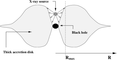
Figure 15: Sketch of an irradiated geometrically-thick accretion disk. Reprocessing does not occur at $R>R_{\mathrm{max}}$

7.4 The nature of the $\cal{R}$ component

Whether we take the ${\cal R}^{\mathrm{min}}$ or the ${\cal R}^{\mathrm{max}}$ assumption, the shape of the $\cal{R}$ component is very different. The spectral index of its ultraviolet part increases from 0.8 to 2.7, the softest spectrum being obtained with the ${\cal R}^{\mathrm{min}}$ assumption. Whatever its normalization, the light curve of the $\cal{R}$ component is similar to the one shown in Fig. 8. The large range of possible spectral shapes prevents us from obtaining strong evidence for any particular models from the spectral shape alone. We therefore have to find additional clues from the other properties of 3C 273.

The BATSE instrument aboard the Compton-GRO satellite monitors quasi-continuously 3C 273 in the 20-200 keV domain since 1991. The light curve can be seen in Fig. 7 of Türler et al. (1998); it shows similarities with the one of the $\cal{R}$ component: There is a maximum in 1994, and variability on time scales of a few years (obviously limited by the “youth” of BATSE) dominates short-time-scale variability. We shall give two tentative interpretations on the basis of this observation.

7.4.1 Reprocessing of X-ray radiation on cold matter

The similarity of the light curves of the $\cal{R}$ component allows us to exclude a viscously-heated accretion disk as the origin of the $\cal{R}$ component. However, reprocessing of hard X-ray radiation on an accretion disk can explain both this similarity, and the correlation between the $\cal{R}$ component light curve and the BATSE light curve. As an iron line has been detected around 6.5 keV Turner et al. (1990), we know that some reprocessing on cold material must take place in 3C 273, and the $\cal{R}$ component seems to be a very good candidate. On the other hand, the absence of reflection hump Maisack et al. (1992) shows that the reprocessed radiation cannot be very important.

The “standard” reprocessing picture already invoked for the $\cal{B}$ component (see Sect. 7.3.5) can account for the spectral energy distribution of the ${\cal R}^{\mathrm{max}}$ component, if an X-ray source of about $10^{47.5}$ ergs s^-1 is located at 60 R_S above the disk, assuming that the mass of the central black hole is $10^{9}$ M_⊙. The disk need not be truncated. This model has however an important drawback. The variability of the $\cal{R}$ component is larger (in term of flux difference) in the infrared domain (J, H, and K bands) than in the optical and ultraviolet domains, while the opposite is expected from the above model; moreover, the disk becomes very large, and variability should not be simultaneous anymore.

7.4.2 The hidden blazar

3C 273 is usually classified as a blazar, because of its radio and gamma-ray properties. Actually its spectral distribution below 100 $\mu$m (and, although to a somehow lesser extent, above 10 keV) is very close (both in spectral shape and in intensity) to the one of 3C 273’s close friend, 3C 279 (cf. Fig. 8 from Von Montigny et al. (1997) and Fig. 1 from Maraschi et al. (1994)). 3C 273 however largely dominates 3C 279 in the blue-bump domain, but their spectral shapes are so different that there is little doubt that one observes different components in both objects. One can therefore easily admit that the component that emits optical radiation in 3C 279 should also be present in 3C 273. Thus the $\cal{R}$ component is possibly the signature of the “blazar 3C 273” in the optical-to-ultraviolet domain.

Models of blazar spectral energy distribution – like synchrotron self-Compton (SSC), external Compton, and proton-initiated cascade – predict a synchrotron radiation component in the optical emission. Therefore, the $\cal{R}$ component – at least in the SSC model – should be correlated to the hard X-ray emission. The synchrotron component in 3C 273 should be much more important than in 3C 279 to account for the $\cal{R}$ component, which appears quite possible considering the numerous free parameters in these models. There is actually a very strong evidence that synchrotron radiation contributes to the optical emission of 3C 273: the optical flux can have a polarization as high as 2.5 % De Diego et al. (1992). Moreover the polarized spectrum is flat in the optical domain, which corresponds well to the $\cal{R}$ spectral energy distribution. If the $\cal{R}$ component is emitted by synchrotron radiation, the extension of the $\cal{R}$ component down to the infrared domain is expected, and the large amplitude of the $\cal{R}$ component variability is not a problem anymore.

8 Summary and possible scenario

As a result of a time series analysis of 29 optical and ultraviolet light curves of 3C 273, we arrive at the conclusion that two components, written here $\cal{B}$ (for “Blue”) and $\cal{R}$ (for “Red”), contribute to the optical and ultraviolet emission. While the relative strength of these components cannot be accurately determined, the $\cal{R}$ component dominates at optical wavelengths, and the relative contribution of the $\cal{B}$ component increases quickly towards short wavelengths.

The $\cal{B}$ component has the interesting property of varying only on time scales shorter than 2 years, independently of the wavelength. If this feature is interpreted in terms of discrete-event models, which would naturally explain the presence of a low-frequency cut-off, the event rate is of the order of 10 per years, and each of them liberates some $10^{52}$ erg, if this component is also responsible for the soft-excess emission. The spectrum of the $\cal{B}$ component including the soft-excess emission is best explained by thermal bremsstrahlung emission, provided that the emitting medium becomes optically thick around $10^{15}$ Hz, and by reprocessing on a (probably geometrically-thick) accretion disk. The fine tuning of the free-free opacity may however be an argument against thermal bremsstrahlung emission, as is the difficulty of instantaneously radiatively heating a zone with a high Thompson scattering opacity. The presence or absence of bound-free and bound-bound transitions in the soft X-ray emission of 3C 273 is a fundamental test within the capabilities of the XMM and AXAF telescopes. We find also that the longer wavelength light curves follow those at shorter wavelengths with a delay. Its amplitude is of the order of 4 days for two light curves whose wavelength ratio is 2. This is very well accounted for by reprocessing on an accretion disk. The explanation is less obvious in the case of thermal bremsstrahlung, but it might be due to the heating or cooling time of the emitting medium.

The $\cal{R}$ component varies on long time scales, larger than those that can be investigated by the time span of our observations. It contributes significantly in the infrared domain, where the amplitude of its variability is larger than in the optical and ultraviolet domain. The BATSE light curve also shows a good morphological resemblance with that of the $\cal{R}$ component. The only viable explanation that we have been able to propose for the origin of the $\cal{R}$ component is the emission from the “blazar 3C 273”, a component that has the same origin as the optical and ultraviolet emission of 3C 279. This has the consequence that the hard X-ray emission of 3C 273 observed from the Earth is not the same as the hard X-ray emission seen by the accretion disk, if reprocessing is to explain the $\cal{B}$ component.

While we do not pretend to understand the extremely complex behaviour of 3C 273, we can propose a picture that can explain qualitatively the optical-to-X-ray emission of 3C 273:

• The ingredients are a supermassive black hole, a geometrically-thick accretion disk, a hard X-ray source located inside the funnel, and a jet perpendicular to the disk.

• A hard X-ray source irradiates the accretion disk, which emits the $\cal{B}$ component from the optical domain up to the soft X-ray domain. The reprocessing features are considerably attenuated because of the reprocessing geometry.

• If the emission from the accretion disk is removed, one sees the “blazar 3C 273”, i.e. the emission from the jet. This is the $\cal{R}$ component. It dominates the spectral energy distribution of 3C 273 at long wavelengths (since the far-infrared domain), but also in the hard X-ray domain. It may be explained by a SSC model.

Seyfert galaxies can be easily linked to the above scenario, if the $\cal{R}$ component can be suppressed. If they have smaller accretion-rate-to-Eddington-accretion-rate ratios, their accretion disks are thinner, which would imply that the curvature detected in the $\cal{B}$ component would be absent.

References

- Barvainis (1987) Barvainis R., 1987, ApJ 320, 537
- Barvainis (1993) Barvainis R., 1993, ApJ 412, 513
- Collier et al. (1998) Collier S.J., Horne K., Kaspi S., et al., 1998, ApJ 500, 162
- Collin-Souffrin (1991) Collin-Souffrin S., 1991, A&A 249, 344
- Collin-Souffrin et al. (1996) Collin-Souffrin S., Czerny B., Dumont A.M. & Zycki P.T., 1996, A&A 314, 393
- Courvoisier & Clavel (1991) Courvoisier T.J.-L. & Clavel J., 1991, A&A 248, 389
- Courvoisier et al. (1988) Courvoisier T.J.-L., Robson E.I., Hughes D.H., Blecha A. & Bouchet P., 1988, Nat 335, 330
- Courvoisier et al. (1990) Courvoisier T.J.-L., Robson E.I., Blecha A., et al., 1990, A&A 234, 73
- Courvoisier et al. (1996) Courvoisier T.J.-L., Paltani S. & Walter R., 1996, A&A 308, L17
- Czerny & Elvis (1987) Czerny B. & Elvis M., 1987, ApJ 321, 305
- De Diego et al. (1992) De Diego J.A., Perez E., Kidger M.R. & Takalo L.O., 1992, ApJ 396, L19
- Edelson & Krolik (1988) Edelson R.A. & Krolik J.H., 1988, ApJ 333, 646
- Galeev et al. (1979) Galeev A.A., Rosner R. & Vaiana G.S., 1979, ApJ 229, 318
- Gaskell & Peterson (1987) Gaskell C.M. & Peterson B.M., 1987, ApJS 65, 1
- Gronenschild & Mewe (1978) Gronenschild E.H.B.M. & Mewe R., 1978, A&AS 32, 283
- Haardt & Maraschi (1991) Haardt F. & Maraschi L., 1991, ApJ 380, L51
- Haardt et al. (1994) Haardt F., Maraschi L. & Ghisellini G., 1994, ApJ 432, L95
- Kunkel (1967) Kunkel W.E., 1967, AJ 72, 1341
- Litchfield et al. (1995) Litchfield S.J., Robson E.I. & Hughes D.H., 1995, A&A 300, 385
- Loska & Czerny (1997) Loska Z. & Czerny B., 1997, MNRAS 284, 946
- Madau (1988) Madau P., 1988, ApJ 327, 116
- Maisack et al. (1992) Maisack M., Kendziorra E., Mony B., et al., 1992, A&A 262, 433
- Maraschi et al. (1994) Maraschi L., Grandi P., Urry C.M., et al., 1994, ApJ 435, L91
- Matt et al. (1993) Matt G., Fabian A.C. & Ross R.R., 1993, MNRAS 264, 839
- Nayakshin & Melia (1997) Nayakshin S. & Melia F., 1997, ApJ 484, L103
- Paltani (1996) Paltani S., 1996, Ph.D. thesis, Geneva University
- Paltani & Courvoisier (1997) Paltani S. & Courvoisier T.J.-L., 1997, A&A 323, 717
- Paltani & Walter (1996a) Paltani S. & Walter R., 1996a, A&A 312, 55 – PW96
- Paltani & Walter (1996b) Paltani S. & Walter R., 1996b. In: Rodonò M. & Catalano S. (eds), Highlights of European Astrophysics, Mem. Soc. Astron. Ital. 67, 1013
- Paltani et al. (1998) Paltani S., Courvoisier T.J.-L., Türler M. & Walter R., 1998. In: Scarsi L., Bradt H., Giommi P., & Fiore F. (eds), The Active X-ray Sky: Results from BepppoSAX and Rossi-XTE, To appear in Nuclear Physics B Proc. Suppl.
- Pelt et al. (1994) Pelt J., Hoff W., Kayser R., Refsdal S. & Schramm T., 1994, A&A 286, 775
- Press (1978) Press W.H., 1978, Comm. Astroph. 7, 103
- Press et al. (1992a) Press W.H., Rybicki G.B. & Hewitt J.N., 1992, ApJ 385, 404
- Press et al. (1992b) Press W.H., Teukolsky S.A., Vetterling W.T. & Flannery B.P., 1992, Numerical Recipes in FORTRAN, 2nd edition, CUP
- Robson et al. (1993) Robson E.I., Litchfield S.J., Gear W.K., et al., 1993, MNRAS 262, 249
- Rokaki et al. (1992) Rokaki E., Boisson C. & Collin-Souffrin S., 1992, A&A 253, 57
- Rokaki et al. (1993) Rokaki E., Collin-Souffrin S. & Magnan C., 1993, A&A 272, 8
- Ross & Fabian (1993) Ross R.R. & Fabian A.C., 1993, MNRAS 261, 74
- Ross et al. (1992) Ross R.R., Fabian A.C. & Mineshige S., 1992, MNRAS 258, 189
- Rybicki & Lightman (1979) Rybicki G.B. & Lightman A.P., 1979, Radiative Processes in Astrophysics, John Wiley & Sons
- Savage & Mathis (1979) Savage B.D. & Mathis J.S., 1979, ARA&A 17, 73
- Shakura & Sunyaev (1973) Shakura N.I. & Sunyaev R.A., 1973, A&A 24, 337
- Simonetti et al. (1985) Simonetti J.H., Cordes J.M. & Heeschen D.S., 1985, ApJ 296, 46
- Terlevich (1992) Terlevich R., 1992. In: Filipenko A.V. (ed.), Relationships between Active Galactic Nuclei and Starburst Galaxies, ASP Conference Series 31, 133
- Türler et al. (1998) Türler M., Paltani S., Courvoisier T.J.-L., et al., 1998, A&AS in press
- Turner et al. (1990) Turner M.J.L., Williams O.R., Courvoisier T.J.-L., et al., 1990, MNRAS 244, 310
- Ulrich et al. (1993) Ulrich M.-H., Courvoisier T.J.-L. & Wamsteker W., 1993, ApJ 411, 125
- Von Montigny et al. (1997) Von Montigny C., Aller H., Aller M., et al., 1997, ApJ 483, 161
- Walter & Fink (1993) Walter R. & Fink H.H., 1993, A&A 274, 105
- Walter et al. (1994) Walter R., Orr A., Courvoisier T.J.-L., et al., 1994, A&A 285, 119
- Wanders et al. (1997) Wanders I., Peterson B.M., Alloin D., et al., 1997, ApJS 113, 69
- White & Peterson (1994) White R.J. & Peterson B.M., 1994, PASP 106, 879
- Yaqoob et al. (1994) Yaqoob T., Serlemitsos P., Mushotzky R., et al., 1994, PASJ 46, L49