THE COSMIC RAY ANTIPROTON SPECTRUM AND A LIMIT FERMILAB-PUB-98/265-A UF-IFT-HEP-98-13   ON THE ANTIPROTON LIFETIME

Abstract

Measurements of the cosmic ray $\overline{p}/p$ ratio are compared to predictions from an inhomogeneous leaky box model of Galactic secondary $\overline{p}$ production combined with an updated heliospheric model that modulates the predicted fluxes measured at the Earth. The heliospheric corrections are crucial for understanding the low–energy part of the spectrum. The $\overline{p}$ production-propagation-modulation model agrees with observations. Adding a finite $\overline{p}$ lifetime to the model, we obtain the limit $\tau_{\overline{p}}>$ 1.7 Myr (90% C.L.). Restrictions on heliospheric properties and the cutoff of low-energy interstellar cosmic rays are discussed.

Submitted to Physical Review Letters

In recent years the presence of antiprotons $(\overline{p}$’s) in the cosmic ray (CR) flux incident upon the Earth has been firmly established by a series of balloon–borne experiments [5, 6, 7, 8, 9, 10, 11, 12, 13]. The CR $\overline{p}/p$ ratio has been measured from kinetic energies of $\sim$ 100 MeV to $\sim$ 19 GeV. The measurements are summarized in Table 1. The CR $\overline{p}/p$ spectrum can be predicted using the Leaky Box Model (LBM) [14, 15, 16], which assumes that the $\overline{p}$’s originate from proton interactions in the interstellar (IS) medium. The $\overline{p}$’s then propagate within the Galaxy until they “leak out” with the characteristic CR Galactic storage time of about 10 million years (Myr) [17]. To obtain a prediction for the energy-dependent $\overline{p}/p$ ratio at the Earth, the IS spectrum must be corrected for modulation of the $p$ and $\overline{p}$ fluxes as the particles propagate through the heliosphere. Thus, a comparison of the observed $\overline{p}/p$ spectrum with predictions tests the Galactic CR production-propagation model and the relevant heliospheric parameters. In addition, if the $\overline{p}$’s have a lifetime $\tau_{\overline{p}}$ short compared to the Galactic storage time, the observed $\overline{p}$ spectrum will be depleted [5, 6, 14], particularly at low energies. This facilitates an interesting test of CPT invariance, which requires $\tau_{\overline{p}}$ = $\tau_{p}$, where the proton lifetime $\tau_{p}$ is known to exceed ${\cal O}(10^{32})$ yr [18].

In this paper the observed CR $\overline{p}/p$ spectrum is shown to be well–described by the predictions of an improved variant of the LBM, once modulation corrections are included. The data constrain the acceptable heliospheric properties. Extending the LBM to permit an unstable $\overline{p}$, we obtain a limit on $\tau_{\overline{p}}$ significantly more stringent than current laboratory bounds obtained from searches for $\overline{p}$ decays in ion traps [19] and storage rings [20].

In the LBM the only source of IS $\overline{p}$’s is the spallation of CR $p$’s [14, 15, 16]: $pN_{Z}\rightarrow\overline{p}X,$ where $N_{Z}$ is a nucleus of charge $Z$, and $X$ is anything. Realistic elemental abundances of the nuclei in the IS medium are given in refs. [15, 16]. The cross section for $Z$ = 1 (the dominant contribution) has been measured in accelerator experiments [14]. For $Z>$ 1, some assumptions about nuclear physics are required to make use of the $Z$ = 1 data. We have used the “wounded nucleon” picture of [16]. The $\overline{p}$’s are assumed to propagate within the Galaxy until they are lost by one of two processes. The dominant loss process is leakage into intergalactic space. This process also applies to other CRs, including protons. The storage lifetime associated with this leakage mechanism varies with rigidity $P$ and can be inferred from measurements of unstable secondary CR nuclei with known decay halflives. The sub–dominant $\overline{p}$ loss mechanism is $p\overline{p}$ annihilation. The annihilation rate is considerably smaller than the leakage rate. Leakage and annihilation, together with elastic and inelastic scattering of $\overline{p}$’s, are the ingredients of the standard leaky box model (SLBM), in which production and loss are assumed to be in statistical equilibrium.

Our analysis is based on the SLBM of Gaisser and Schaeffer using the parameters of [16], but with a Galactic storage time improved to account for the non-uniform Galactic CR distribution [17]. This inhomogeneous LBM (ILBM) results in a somewhat longer storage time, $4.1\times 10^{14}~{}[1+P/(3{\rm\ GeV})]^{-0.6}$ sec. The uncertainties on the parameters of the ILBM result in uncertainties on the normalization of the predicted $\overline{p}/p$ ratio but, to a good approximation, do not introduce significant uncertainties in the shape of the predicted spectrum. Specifically, uncertainties on four ILBM parameters must be considered: (i) the storage time ($\pm$67% [17]), (ii) the IS primary $p$ flux ($\pm$35% [16]), (iii) the $\overline{p}$ production cross section ($\pm$10% [14, 16]), and (iv) the composition of the IS medium, which introduces an uncertainty of $<6$% on the predicted $\overline{p}$ flux [16]. In the following we neglect the last of these uncertainties since it is relatively small. Within the quoted fractional uncertainties on the other three parameters we treat all values as being a priori equally likely. Note that the predicted $\overline{p}/p$ ratio is approximately proportional to each of the three parameters under consideration.

The curves in Fig. 1 show the ILBM $\overline{p}/p$ spectra for the parameter choices that result in the largest and smallest $\overline{p}/p$ predictions. The predicted IS spectrum does not give a good description of the observed spectrum at the top of the atmosphere. Good agreement is not expected because the CR spectra observed at the Earth are modulated as the particles propagate into the Sun’s magnetic region of influence, the heliosphere [21, 22], which consists of the solar magnetic field ${\bf B}$ and the solar wind. Measurements by the Pioneer 10 and Voyager 1 spacecraft [23] indicate that the outer boundary of the heliosphere (the heliopause) is at heliocentric distance $r_{0}\geq$ 71 astronomical units (AU). Theoretical considerations favor $r_{0}$ = 100–130 AU [21]. Fortunately, the heliospheric corrections to the IS fluxes are not sensitive to variations of $r_{0}$ within these ranges. The wind, which is assumed to blow radially outwards, has an equatorial speed $V_{W}\sim$ 400 km sec^-1. Away from the equatorial plane the Ulysses spacecraft has found $V_{W}\sim$ 750 km sec^-1 [24]. The wind pressure declines until it reaches the IS value at the heliopause. The solar wind plasma (nuclei and $e^{-})$ moves in bulk outwards from the Sun with turbulence that peaks around solar magnetic maximum. The solar wind imposes an energy threshold for IS CRs reaching the Earth. This energy cutoff is much higher for particles coming in along the polar directions where the wind speeds are higher, than along the equatorial route where the wind speeds are lower. The wind also carries the solar magnetic flux outward. Solar rotation $\Omega_{\odot}$ twists the field lines to form a Parker spiral. The smoothed heliomagnetic field ($B_{\oplus}\sim$ 5 nT at the Earth’s orbit) declines as it changes from radial at the Sun to azimuthal in the outer Solar System. The heliomagnetic polarity (${\rm sign}(A)$) is opposite in northern and southern solar hemispheres and switches sign somewhat after sunspot maximum (roughly every 11 years), when the field becomes more disordered. The regions of opposite magnetic polarity are separated by an approximately equatorial, unstable neutral current sheet. The sheet is wavy and spiraled; its waviness is measured by its “tilt” angle $\alpha$, which relaxes from $\simeq$ $50^{\circ}$ at polarity reversal to $\lesssim$ $10^{\circ}$ just before reversal [21, 24, 25, 26].

Cosmic rays enter the heliosphere on ballistic trajectories and are then subject to the forces associated with the wind and solar magnetic field [22, 26]. The propagation of the CRs within the heliosphere is described by a drift-diffusion (Fokker-Planck) equation [27]. The CRs are pushed outwards by the bulk motion of the wind (elastic scattering), lose energy as they perform work on the wind (adiabatic deceleration or inelastic scattering), are diffusively scattered by field turbulence, and execute a drift orthogonal to the curving magnetic field lines as they spiral inwards along the field lines. Particles with $qA>0$ $(<0)$ drift in along a polar (sheet) route. The IS particles with sufficient energy to overcome the various energy losses reach the inner Solar System after being randomly scattered by turbulence.

We compute the modulation of CR fluxes by the method of characteristics and combined Runge-Kutta/Richardson-Burlich-Stoer techniques [28]. The calculation uses the heliospheric transport models of Jokipii et al. [26], combined with the ILBM $\overline{p}$ spectrum, and updated by Pioneer, Voyager, and Ulysses heliospheric measurements [23, 24]. Our calculation includes magnetic curvature drift since older heliospheric models [29] that neglected this drift component have been shown [26] to be inadequate. Note that magnetic drift changes sign for oppositely-charged particles and field polarities, in contrast to diffusion $\kappa$ which is charge-invariant and whose effect partly cancels in the $\overline{p}/p$ ratio. The calculation is simplified by ignoring turbulence where its effects are small, which in practice means everywhere except across the sheet, where for particles with speed $v$, we use: $\kappa_{\perp}$ = $(2-3)\times 10^{17}[B_{\oplus}/B(r)](P/{\rm GeV})^{0.3}(v/c)$ m²/sec [30]. Finally, IS “pickup” ions and solar CRs have been neglected [21, 24].

In the following, we restrict our analysis to the data sets recorded by the MASS91, IMAX, BESS, and CAPRICE experiments (Table 1). These data were recorded in the period 1991–1994, corresponding to a well–behaved part of the solar cycle for which the heliospheric modulation corrections can be calculated with some confidence. In addition, compared to the earlier data, these more recent data sets benefited from detectors with improved particle identification and hence lower backgrounds. In Fig. 2 the measurements are compared with the predictions for a stable antiproton, taking the central parameter values for our ILBM calculation and three different sets of heliospheric corrections (lower, central, and upper). The corresponding heliospheric parameters are (a) Lower: equatorial $V_{W}=$ 375 km sec^-1, polar $V_{W}=$ 700 km sec^-1, $B_{\oplus}=$ 4.0 nT; (b) Central: equatorial $V_{W}=$ 400 km sec^-1, polar $V_{W}=$ 750 km sec^-1, $B_{\oplus}=$ 4.5 nT; and (c) Upper: equatorial $V_{W}=$ 425 km sec^-1, polar $V_{W}=$ 800 km sec^-1, $B_{\oplus}=$ 5.0 nT. Note that for each parameter set there are four curves, corresponding to the calculated heliospheric corrections at the dates of each of the four balloon flights. Given the variation of the predicted ratios with heliospheric parameter choice, we conclude that the predictions are able to give a good description of the data, and that there is no significant evidence for a short antiproton lifetime. Note that (i) for a given set of parameters, the heliospheric corrections are similar for the BESS, IMAX, CAPRICE, and MASS91 data, with appreciable differences only at the lowest kinetic energies; and (ii) in the region above $\sim 3$ GeV, the differences between the predictions corresponding to the different choices of heliospheric parameters are small compared to the statistical errors on the data. However, in the lowest energy region, below $\sim 700$ MeV, there are significant differences in the predictions for the three different choices of heliospheric parameters. Hence, in the fitting procedure employed to extract an upper limit on $\tau_{\overline{p}}$, we must allow the overall normalization of the predictions to vary to account for the uncertainties arising from the choice of the ILBM parameters, and the heliospheric parameters to vary to account for the sensitivity of the low-energy $\overline{p}/p$ ratio to these parameters.

To obtain a limit on $\tau_{\overline{p}}$ we add to the ILBM one additional loss mechanism, $\overline{p}$ decay. Note that the $\overline{p}$ lifetime must be $<{\cal O}(10)$ Myr to significantly distort the $\overline{p}$ spectrum. However, this timescale is much longer than the lifetime sensitivity of existing laboratory searches for $\overline{p}$ decay [20]. The results from maximum likelihood fits to the BESS, IMAX, CAPRICE, and MASS91 measurements are shown in the inset of Fig. 2 as a function of the assumed $\tau_{\overline{p}}$ for eight heliospheric parameter sets F1 – F8. The F1 parameters are equatorial (polar) $V_{W}$ = 375 (700) km sec^-1, and $B_{\oplus}$ = 4.0 nT. The values for the equatorial (polar) $V_{W}$ and $B_{\oplus}$ increase for the other parameter sets in steps of respectively 5 (10) km sec^-1 and 0.1 nT. Hence, the parameters for F8 are equatorial (polar) $V_{W}$ = 410 (770) km sec^-1, and $B_{\oplus}$ = 4.7 nT. The fits, which take account of the Poisson statistical fluctuations on the number of observed events and the background subtraction for each data set (Table 1), also allow the normalization of the ILBM predictions to vary within the acceptable range (Fig. 1). The best maximum likelihood fits correspond to the heliospheric parameter sets F4 and F5, and are consistent with a completely stable antiproton. The extreme parameter sets (F1 and F8) are excluded at $>90$% C.L. for all values of $\tau_{\overline{p}}$, and hence the data constrain the heliospheric parameters. In particular, the following parameter ranges are preferred: equatorial $V_{W}$ = 375–410 km sec^-1, polar $V_{W}$ = 700–770 km sec^-1, and $B_{\oplus}$ = 4.0–4.7 nT. Finally, the fits do not favor values of $\tau_{\overline{p}}<{\cal O}(1)$ Myr. We obtain the bounds:

$$\tau_{\overline{p}}\quad>\quad 1.7\ {\rm Myr\ \ (90\%\ C.L.)}\quad,\quad 1.1\ {\rm Myr\ \ (95\%\ C.L.)}\quad,\quad 630\ {\rm kyr\ \ (99\%\ C.L.)}\quad.\\$$ (1)

A new generation of balloon experiments, or a dedicated orbital CR detector such as the recently tested AMS [31], could greatly improve the statistical precision of the measured $\overline{p}$ spectrum. This would facilitate more significant bounds on the heliospheric parameters, and enable a search for exotic sources of $\overline{p}$’s, particularly at low kinetic energies $K$. However we note that, neglecting diffusion, the solar wind cuts off the polar–routed flux at $K_{\oplus}$ = 0.26–0.40 GeV (mass-independent cutoff rigidity scaling approximately as $qB_{\oplus}V^{2}_{W}$). Particles with these threshold energies at the Earth have IS energies $K_{\rm IS}$ = 0.54–0.80 GeV. In contrast, the sheet-routed flux exhibits no significant cutoff. Noting that in the present solar cycle the protons reach the Earth via the polar route, and $\overline{p}$’s reach the Earth via the sheet route, we conclude that when the next solar cycle begins (around 2003) new experiments will only be sensitive to IS $\overline{p}$’s with $K_{\rm IS}\gtrsim 0.5$ GeV.

In summary, with an inhomogeneous LBM of IS $\overline{p}$ production and propagation, together with a calculation of heliospheric corrections that includes up–to–date data on the solar wind, we obtain good agreement with the observed CR $\overline{p}/p$ ratio. Extending the ILBM model to permit a finite $\tau_{\overline{p}}$ we obtain lower limits on $\overline{p}$ decay that are more stringent than laboratory bounds. Our fits also constrain the ranges of the heliospheric parameters. We note that in the next solar cycle the effective cutoff in detectable low energy IS $\overline{p}$’s will be significantly higher than at present, which will decrease the sensitivity of experiments searching for exotic sources of antiprotons.

Acknowledgements

It is a pleasure to thank Thomas Gaisser, J. R. Jokipii, and E. J. Smith for their insights. This work was supported at Fermilab under grants U.S. DOE DE-AC02-76CH03000 and NASA NAG5-2788. and at the U. Florida, Institute for Fundamental Theory, under grant U.S. DOE DE-FG05-86-ER40272.

Experiment		Field	Flight	KE Range	Cand-	Back-	Observed	predict-
		Pol.	Date	(GeV)	idates	ground	$\overline{p}/p$ Ratio	tion
Golden†	[5]	$+$	June 1979	5.6 – 12.5	46	18.3	$(5.2\pm 1.5)\times 10^{-4}$	-
Buffington†	[32]	${\rm n/a}$	June 1980	0.13 – 0.32	17	3.0	$(2.2\pm 0.6)\times 10^{-4}$	-
Bogomolov†	[6]	$+$	1972-1977	2.0 – 5.0	2	-	$(6\pm 4)\times 10^{-4}$	-
Bogomolov‡	[7]	$-$	1984-1985	0.2 – 2.0	1	-	$(6^{+14}_{-5})\times 10^{-5}$	-
Bogomolov‡	[8]	$-$	1986-1988	2.0 – 5.0	3	-	$(2.4^{+2.4}_{-1.3})\times 10^{-4}$	-
PBAR†	[33]	$-$	Aug. 1987	0.205 – 0.64	n/a	n/a	$\leq 4.6\times 10^{-5}$	-
PBAR†	[34]	$-$	Aug. 1987	0.10 – 0.64	n/a	n/a	$\leq 2.8\times 10^{-5}$	-
PBAR†	[34]	$-$	Aug. 1987	0.64 – 1.58	n/a	n/a	$\leq 6.1\times 10^{-5}$	-
LEAP†	[35]	$-$	Aug. 1987	0.12 – 0.86	n/a	n/a	$\leq 1.8\times 10^{-5}$	-
MASS91	[9]	$+$	Sep. 1991	3.70-19.08	11	3.3	$(1.24^{+0.68}_{-0.51})\times 10^{-4}$	$1.3\times 10^{-4}$
IMAX	[10]	$+$	July 1992	0.25 – 1.0	3	0.3	$(3.14^{+3.4}_{-1.9})\times 10^{-5}$	$1.2\times 10^{-5}$
IMAX	[10]	$+$	July 1992	1.0 – 2.6	8	1.9	$(5.36^{+3.5}_{-2.4})\times 10^{-5}$	$6.2\times 10^{-5}$
IMAX	[10]	$+$	July 1992	2.6 – 3.2	5	1.2	$(1.94^{+1.8}_{-1.1})\times 10^{-4}$	$1.1\times 10^{-4}$
BESS	[11]	$+$	July 1993	0.20 – 0.60	6	$\sim 1.4$	$(5.2^{+4.4}_{-2.8})\times 10^{-6}$	$6.4\times 10^{-6}$
CAPRICE	[13]	$+$	Aug. 1994	0.6 – 2.0	4	1.5	$(2.5^{+3.2}_{-1.9})\times 10^{-5}$	$3.3\times 10^{-5}$
CAPRICE	[13]	$+$	Aug. 1994	2.0 – 3.2	5	1.3	$(1.9^{+1.6}_{-1.0})\times 10^{-4}$	$1.1\times 10^{-4}$

TABLE I.: Summary of cosmic ray antiproton results. Listed from left to right are the experiments, solar cycle polarity (note: minimum-to-minimum solar cycles 20:1964.6–1976.5, 21:1976.5–1986.7, and 22:1986.7–1996.3), balloon flight date, $\overline{p}$ kinetic energy range, number of $\overline{p}$ candidates observed, estimated number of background events, measured $\overline{p}/p$ ratio at the top of the atmosphere, and the ILBM prediction using the heliospheric parameters: equatorial (polar) $V_{W}$ = 395 (740) km sec^-1, $B_{\oplus}$ = 4.4 nT. † Not shown in Fig. 1 or used in analysis. ‡ Not used in analysis.

FIG. 1.: Observed $\overline{p}/p$ ratio at the top of Earth atmosphere (see Table 1). The solid curves show the upper and lower interstellar ratios predicted by the ILBM described in the text, without solar modulation. The broken curve shows the ILBM prediction with the same parameters used for the modulated predictions of Fig. 2.

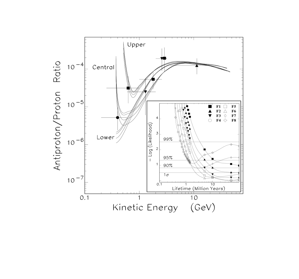
FIG. 2.: Observed $\overline{p}/p$ ratio at the top of Earth atmosphere compared with the ILBM predictions (see Fig. 1) after heliospheric modulation. The upper, central, and lower families of curves correspond to the upper, central, and lower heliospheric parameter sets described in the text. For each heliospheric parameter set there are four curves corresponding to the epochs of the four balloon flights (at low energies, from top to bottom: MASS91, IMAX, BESS, CAPRICE). The inset shows the fit results as a function of the assumed $\tau_{\overline{p}}$ for the eight heliospheric parameter sets (F1 – F8) described in the text.

REFERENCES

- [1]
- [2]
- [3] E-mail: sgeer@fnal.gov.
- [4] E-mail: kennedy@phys.ufl.edu.
- [5] R.L. Golden et al., Phys. Rev. Lett. 43, 1196 (1979).
- [6] E.A. Bogomolov et al., Proc. ICRC, Kyoto 1, 330 (1979).
- [7] E.A. Bogomolov et al., Proc. ICRC, Moscow 2, 72 (1987).
- [8] E.A. Bogomolov et al., Proc. ICRC, Adelaide 3, 288 (1990).
- [9] M. Hof et al., Astrophys. J. 467, L33 (1996).
- [10] J.W. Mitchell et al., Phys. Rev. Lett. 76, 3057 (1996).
- [11] A. Moiseev et al., Astrophys. J. 474, 479 (1997).
- [12] K. Yoshimura et al., Phys. Rev. Lett. 75, 3792 (1995).
- [13] M. Boezio et al., Astrophys. J. 487, 415 (1997).
- [14] S. A. Stephens, Astrophys. Space Sci. 76, 87 (1981); S. A. Stephens and R. L. Golden, Space Sci. Rev. 46, 31 (1987).
- [15] W. R. Webber and M. S. Potgieter, Astrophys. J. 344, 779 (1989).
- [16] T. K. Gaisser and R. K. Schaefer, Astrophys. J. 394, 174 (1992).
- [17] W. R. Webber et al., Astrophys. J. 390, 96 (1992); P. Chardonnet et al., Phys. Lett. B384, 161 (1996).
- [18] C. Caso et al. (Particle Data Group), Euro. Phys. J. C3, 613 (1998).
- [19] G. Gabrielse et al. (Antihydrogen Trap Collab.), CERN proposal CERN-SPSLC-96-23 (1996).
- [20] S. Geer et al., Phys. Rev. D50, 1680 (1994); M. Hu et al. (APEX Collab.), FERMILAB-PUB-98/216-E, submitted to Phys. Rev. Lett.
- [21] M. Stix, The Sun: An Introduction (Berlin: Springer-Verlag, 1989); T. Encrenaz et al., The Solar System, 2nd ed. (Berlin: Springer-Verlag, 1990). R. Howard, Ann. Rev. Astron. Astrophys., 22, 131 (1984). The wavy sheet’s locus in polar co-ordinates is = 0.
- [22] M. S. Longair, High Energy Astrophysics, 2 vols., 2nd ed. (Cambridge: Cambridge University Press, 1992).
- [23] Pioneer 10/11 http://spaceprojects.arc.nasa.gov/Space_Projects/pioneer/PNhome.html; Voyager 1/2 http://vraptor. jpl.nasa.gov/ .
- [24] E. J. Smith, R. G. Marsden et al., Science 268, 1005ff. (1995); J. Kóta and J. R. Jokipii, ibid., 1024; R. G. Marsden, E. J. Smith et al., Astron. Astrophys. 316, 279ff. (1996); Ulysses http://ulysses.jpl.nasa.gov/ .
- [25] National Solar Observatory http://www.nso.noao.edu/pub/sunspots .
- [26] J. R. Jokipii and D. A. Kopriva, Astrophys. J. 234, 384 (1979); J. R. Jokipii and P. A. Isenberg, Astrophys. J. 234, 746 (1979); 248, 845 (1981); J. R. Jokipii and B. Thomas, Astrophys. J. 243, 1115 (1981); J. R. Jokipii and J. M. Davila, Astrophys. J. 248, 1156 (1981);
- [27] H. Risken, The Fokker-Planck Equation: Methods of Solution and Applications (New York: Springer-Verlag, 1984).
- [28] E. C. Zachmanoglou and D. W. Thoe, Introduction to Partial Differential Equations with Applications (New York: Dover Publications, 1986); W. H. Press et al., Numerical Recipes in C: The Art of Scientific Computing, 2nd ed. (Cambridge: Cambridge University Press, 1992).
- [29] L. J. Gleeson and W. I. Axford, Astrophys. J. 149, L115 (1967); Astrophys. J. 154, 1011 (1968); L. A. Fisk and W. I. Axford, J. Geophys. Res. 74, 4973 (1969); L. A. Fisk, J. Geophys. Res. 76, 221 (1971).
- [30] Note that would be smaller around solar maximum.
- [31] S. Ahlen et al. (AMS Collab.), Nucl. Instrum. Meth. A350, 351 (1994); http://hpamsmi2.mi.infn.it/ ~wwwams/A_AMS.html .
- [32] A. Buffington et al., Astrophys. J. 248, 1179 (1981).
- [33] S.P. Ahlen et al., Phys. Rev. Lett. 61, 145 (1988).
- [34] M.H. Salamon et al., Astrophys. J. 349, 78 (1990).
- [35] R.E. Streitmatter et al., Proc. ICRC, Adelaide 3, 277 (1990).