Biasing and high-order statistics from the SSRS2

Abstract

We analyze different volume–limited samples extracted from the Southern Sky Redshift Survey (SSRS2), using counts–in–cells to compute the Count Probability Distribution Function (CPDF).From the CPDF we derive volume–averaged correlation functions to fourth order and the normalized skewness and kurtosis $S_{3}=\bar{\xi_{3}}/\bar{\xi_{2}}^{2}$ and $S_{4}=\bar{\xi_{4}}/\bar{\xi_{2}}^{3}$. We find that the data satisfies the hierarchical relations in the range $0.3~{}\hbox to0.0pt{$<$\hss}{\lower 4.30554pt\hbox{$\sim$}}\bar{\xi_{2}}~{}\hbox to0.0pt{$<$\hss}{\lower 4.30554pt\hbox{$\sim$}}10$. In this range, we find $S_{3}$ to be scale-independent with a value of $\sim 1.8$, in good agreement with the values measured from other optical redshift surveys probing different volumes, but significantly smaller than that inferred from the APM angular catalog. In addition, the measured values of $S_{3}$ do not show a significant dependence on the luminosity of the galaxies considered. This result is supported by several tests of systematic errors that could affect our measures and estimates of the cosmic variance determined from mock catalogs extracted from N-body simulations. This result is in marked contrast to what would be expected from the strong dependence of the two-point correlation function on luminosity in the framework of a linear biasing model. We discuss the implications of our results and compare them to some recent models of the galaxy distribution which address the problem of bias.

1 Introduction

One of the simplest measures of clustering is the two-point correlation function. However, it provides a complete description only in the case of a Gaussian distribution. The complexity of the large-scale clustering pattern of galaxies (large voids, great walls, groups, clusters) reveals non-Gaussian features that cannot be fully described by second order statistics. Instead, a distribution of $N$ objects can only be fully described by its series of $N$-point correlation functions or alternatively, by the entire set of count probabilities $P(N,V)$, i.e. the probability of finding $N$ objects in a randomly placed volume $V$. This set defines the count probability distribution function, hereafter CPDF.

Direct calculation of the two, three and four-point correlation functions on galaxy catalogs has shown that the few-body correlations on mildly non-linear scales (i.e., from $\sim 1$ to a few $h^{-1}Mpc$) can be expressed as a sum of products of two-point correlation functions:

$$\xi_{3}(r_{1},r_{2},r_{3})=Q[\xi_{2}(r_{1})\xi_{2}(r_{2})+\xi_{2}(r_{2})\xi_{2}(r_{3})+\xi_{2}(r_{1})\xi_{2}(r_{3})],$$ (1)

with values of $Q$ in the range 0.8 to 1.3 (e.g., Groth & Peebles 1977, Fry & Seldner 1982, Efstathiou & Jedredjewski 1984). This relation has been generalized to the $N$-point correlation function of the matter distribution, defining a set of hierarchical models (Fry 1984a, Schaeffer 1984):

$$\xi_{J}({\mathbf{r}}_{1},...,{\mathbf{r}}_{J})=\sum_{\alpha}Q_{J}^{(\alpha)}\sum_{ij}\prod^{J-1}\xi_{2}(r_{ij}),$$ (2)

where the $Q_{J}^{(\alpha)}$ are independent of the scale and $\alpha$ denotes each irreducible geometrical configuration of $J$-points. In general $Q_{J}$ depends on the shape of the $J$-tuple $({\mathbf{r}}_{1},...,{\mathbf{r}}_{J})$, although the dependence in the case of $Q_{3}$ should be fairly weak (Fry 1984b). These hierarchical models can also be characterized by the volume-averaged correlation functions $\bar{\xi}_{J}=V^{-J}\int_{V}\xi_{J}d^{3}r_{1}...d^{3}r_{J}$ through the relation:

$$\bar{\xi}_{J}(r)=S_{J}\bar{\xi_{2}}^{J-1}(r),$$ (3)

where the coefficients $S_{J}$ are independent of the scale and are related to the previously defined $Q_{J}$ by (Balian & Schaeffer 1989):

$$S_{J}=B_{J}J^{J-2}Q_{J}.$$ (4)

The $B_{J}$ are geometrical factors close to 1, which depend on the shape of $\xi(s)$.

The hierarchical relation (??) is a solution of the BBGKY equations in the strongly non-linear regime and is also predicted in the linear regime, as shown by using perturbation theory (e.g., Juszkiewicz, Bouchet & Colombi 1993). However, the value of $Q_{J}$ ($S_{J}$) may differ in the different regimes. Therefore, an important question is whether this hierarchical relation is satisfied by the mass distribution and on what range of scales it is valid. This also raises the problem of how to relate these predictions for the mass fluctuations to the observed galaxy distribution, namely the nature of the biasing process.

In order to further investigate these issues we analyze the clustering properties of galaxies using the Southern Sky Redshift Survey (SSRS2, da Costa et al. 1994, 1998). Its depth, dense sampling and geometry make it one of the most suitable samples currently available to study high order statistics over a wide range of scales. In previous papers (Benoist et al. 1996, hereafter paper i, Cappi et al. 1998), we have used the SSRS2 catalog to investigate the dependence of galaxy clustering on luminosity and the nature of galaxy bias using second order statistics. In the present paper we extend our work to higher order investigating the behavior of the skewness $S_{3}$ and the kurtosis $S_{4}$ as functions of luminosity. In particular, we address the following questions: 1) the validity of the hierarchical relations; 2) the range of scales over which these relations are satisfied ; 3) the nature of bias based on the properties of higher order moments, more specifically the skewness.

These issues have been addressed in different papers. For instance, Bouchet et al. (1993) have examined the validity of the hierarchical relations using the 1.2 Jy IRAS redshift survey. However, this sample under-represents high density regions and does not adequately probe nonlinear clustering, because of the low density of galaxies. The use of the skewness and kurtosis to probe the nature of biasing was investigated by Gaztañaga and Frieman (1994), using the two-dimensional APM galaxy survey.

In section 2 we briefly describe the data and the various sub-samples used in the present analysis. We also present the CPDF derived from the SSRS2 and compare them to various analytical models that have been proposed to describe the observed clustering properties of galaxies. In section 3, we compute the volume averaged correlation functions up to the fourth order and examine the validity of the hierarchical model. We also derive the skewness and the kurtosis for the various sub-samples. In section 4, we investigate the dependence of the skewness on the luminosity, examining possible sources of errors in its determination. In section 5. these results are compared to the predictions of different galaxy biasing models. Finally, in section 6 we summarize our main conclusions.

2 Counts-in-Cells

In the present analysis we use the SSRS2 south sample (da Costa et al. 1994, 1998) which contains about 3600 galaxies brighter than $m_{B}=15.5$, distributed over 1.13 steradians of the southern galactic cap ($b<-40^{o}$) within the declination range $-40^{o}<\delta<-2.5^{\circ}$. Radial velocities have been corrected to the Local Group rest frame (Yahil, Tammann, & Sandage 1977). For comparison we also use the SSRS2 north (da Costa et al. 1998) and CfA2 south samples (Huchra et al. 1997), covering smaller areas ($\sim 0.6$ steradians) in the northern and southern galactic caps, respectively. Even though smaller, these samples are useful to directly gauge the variance of the various statistics.

Since all galaxies in the SSRS2 have been assigned morphological types, following the ESO-Uppsala classification system ($T$), we have adopted a morphological-dependent K-correction, $K(z,T)$, to compute the absolute magnitude, $M$, of a galaxy according to

$$M=m-25-5\log D_{L}-K(z,T),$$ (5)

where $D_{L}$ is the luminosity distance for standard Friedman models:

$$D_{L}=\frac{c}{H_{0}}\frac{1}{q_{0}^{2}}[1-q_{0}+q_{0}z+(q_{0}-1)\sqrt{2q_{0}z+1}].$$ (6)

In the following analysis, we have adopted $H_{0}=100$ and $q_{0}=0.5$. We have divided the sample into four morphological classes and applied for each class the K-correction following Efstathiou, Ellis & Peterson (1988) (see paper i). The analysis presented below has been carried out in redshift space.

We have extracted from the SSRS2 six volume-limited sub-samples as done in paper i. The characteristics of these sub-samples are given in Table ?? which lists: in column (1) the sub-samples id; in column (2) the depth; in column (3) the absolute magnitude limit; in column (4) the number of galaxies; in column (5) the density; in column (6) the correlation length $s_{0}$. Note that the magnitude interval between sub-samples is not a constant because of the strong luminosity segregation observed in paper i for galaxies brighter than $L_{*}$, which requires a finer grid at the bright end.

We have measured $P(N,s)$ as the fraction of randomly placed spheres of radius $s$ containing exactly $N$ galaxies. The probabilities are computed using $10^{6}$ random spheres (in order to have less than $10\%$ error on $P(N,s=1h^{-1}Mpc)$), rejecting those crossing the survey edges. While this procedure limits the number of independent spheres on large scales, it has the advantage of making no assumptions about the galaxy distribution beyond the surveyed volume.

In Figures ??– ?? we show the CPDF computed for the sub-samples D91, D138, and D168 respectively, compared to the predictions of four models: the gravitational quasi-equilibrium (Saslaw & Hamilton 1984, Saslaw et al. 1990, Itoh, Inagaki & Saslaw 1993, Sheth, Mo & Saslaw 1994); the negative binomial (Carruthers & Minh 1983); the log-normal (Coles & Jones 1991); and the Gaussian distribution.

On small scales ($s~{}\hbox to0.0pt{$<$\hss}{\lower 4.30554pt\hbox{$\sim$}}10h^{-1}Mpc$), where significant deviations from Gaussianity are noticeable, all analytical models fit the data equally well over the whole range of $N$, independently of the luminosity class. On larger scales, there is a clear trend towards Gaussianity as examplified in panels (b), (c) and (d) of Figure ??, corresponding to scales in the range $20h^{-1}Mpc~{}\hbox to0.0pt{$<$\hss}{\lower 4.30554pt\hbox{$\sim$}}s~{}\hbox to0.0pt{$<$\hss}{\lower 4.30554pt\hbox{$\sim$}}30h^{-1}Mpc$. Note that in this case all analytical models provide a poor fit for intermediate values of $N$. Unfortunately, several effects plague this comparison and prevent the use of the CPDF to discriminate between models. For fainter samples (figure ??) the volume probed is too small to reach Gaussianity. In other cases, the samples are too dilute to either compute reliable counts or to show significant differences between models. Despite these problems it is still true that using the CPDF can be, in some cases, more informative than quantities related to the moments of the distribution. Since the moments are an integral quantity they have larger errors. It is worth pointing out that the CPDF computed even for the extreme case of sub-sample D168, containing the brightest galaxies, which has the smallest number of galaxies and lowest density, looks comparable to the other more dense sub-samples.

3 Moments of the Counts Distribution

3.1 Relation between Correlation Functions

The volume-averaged correlation functions have been calculated from the counts in cells. The centered moments of order $J$, $\mu_{J}$, can be directly derived from the count probabilities $P(N,s)$ (Peebles 1980):

$$\mu_{J}(s)=\langle(N-\bar{N})^{J}\rangle=\sum_{N=0}^{N_{max}(s)}P(N,s)(N-\bar{N})^{J},$$ (7)

where $N_{max}(s)$ is the maximum number of galaxies counted in a sphere of radius $s$, and $\bar{N}=\sum NP(N)$, i.e. at each scale we have computed directly the effective mean number of galaxies from the counts, and not from simple ratio $N_{gal}/V_{sample}$.

In the case of a smoothed distribution, the volume-averaged correlation functions $\bar{\xi_{J}}=V^{-J}\int_{V}\xi_{J}d^{3}r_{1}...d^{3}r_{J}$ are related to the corresponding cumulants through $\bar{N}^{J}\bar{\xi}_{J}=k_{J}$, where $k_{2}=\mu_{2}$, $k_{3}=\mu_{3}$, $k_{4}=\mu_{4}-3\mu_{2}^{2}$ (Kendal & Stuart 1991). For a discrete distribution, these relations have to be corrected for shot-noise. We assume that our galaxy samples are Poisson realizations of an underlying smooth “galaxy” density field. Thus, we obtain the following relations between the volume-averaged correlation functions and the cumulants of the discrete distribution (Peebles 1980, Fry 1985):

$$\bar{\xi}_{2} = \frac{1}{\bar{N}^{2}}(k_{2}-\bar{N})$$

$$\bar{\xi}_{3} = \frac{1}{\bar{N}^{3}}(k_{3}-3k_{2}+2\bar{N})$$

$$\bar{\xi}_{4} = \frac{1}{\bar{N}^{4}}(k_{4}-6k_{3}+11k_{2}-6\bar{N})$$ (8)

Following this procedure, we have computed the volume-averaged correlation functions up to order 4 for the six volume-limited sub-samples presented in Table ??. $\bar{\xi}_{2}$ is shown in Figure ??, where the change in the amplitude as a function of the luminosity can be easily seen. Here, as well as in the subsequent plots, the error bars correspond to the rms value as measured for 15 bootstrap re-samplings of each sub-sample. We have measured the increase in the amplitude of $\bar{\xi}_{2}(s)$ in the range $2h^{-1}Mpc~{}\hbox to0.0pt{$<$\hss}{\lower 4.30554pt\hbox{$\sim$}}s~{}\hbox to0.0pt{$<$\hss}{\lower 4.30554pt\hbox{$\sim$}}10h^{-1}Mpc$ and derived the relative bias ratios for the different luminosity classes, assuming a linear biasing model. As discussed in paper i the relative bias shows a weak dependence on luminosity for sub-L_∗ galaxies, with a rapid increase at the bright end.

In order to estimate the amplitude of sample-to-sample variations, in Figure ?? we compare $\bar{\xi}_{2}(s)$ for each SSRS2 south sub-sample to those obtained from similar sub-samples extracted from the CfA2 south and SSRS2 north. Note that, for D168 this comparison was not possible because of the small number of bright galaxies in these two catalogs which cover about half of the area surveyed by the SSRS2 south. As it can be seen, within 10$h^{-1}Mpc$ there is a remarkable agreement in the amplitude and shape of the $\bar{\xi}_{2}(s)$ derived from these surveys probing different directions of the sky and different large-scale structures. Most of the differences occur on larger scales, where the results are sensitive to cosmic variance.

For each sub-sample we have also computed the volume-averaged three-point $\bar{\xi}_{3}$, and four-point $\bar{\xi}_{4}$, correlation functions. In Figure ?? these functions are shown as a function of $\bar{\xi}_{2}$ for the six sub-samples considered. Also shown in each panel is the best power-law fit to the data points corresponding to $L_{*}$ galaxies (D91). As predicted by the hierarchical model there is a tight relation between the third and fourth order correlations with $\bar{\xi}_{2}$. Moreover, the slopes of the power-law fits are in good agreement with the expected index $(J-1)$ in the framework of the hierarchical models, as defined by equation (3). For comparison, in Figure ?? we also show the best fit given by Bouchet et al. (1993) for the IRAS galaxies. The comparison between IRAS and SSRS2 galaxies shows that these two populations follow similar relations with comparable amplitudes.

It is worth pointing out that the hierarchical relations hold to relatively large values of the variance ($\bar{\xi}_{2}\sim 10$), corresponding to non-linear scales. It is important to emphasize that the optical data used here gives further support to the original claim of Bouchet et al. (1993) that the hierarchical relation extends to relative non-linear regime, since with the IRAS data scales corresponding to $\bar{\xi}_{2}\sim 10$ could only be probed with a single sub-sample. While this behavior is predicted by perturbation theory for the mildly nonlinear regime, there is currently no compelling theoretical reason to justify this behavior for the non-linear scales probed by the optical data, except that the solution for the BBGKY equations has this property. Some deviations from the scale-invariance are noticeable on small ($\bar{\xi}_{2}~{}\hbox to0.0pt{$<$\hss}{\lower 4.30554pt\hbox{$\sim$}}0.2$) and large scales ($\bar{\xi}_{2}>10$). A key question is to determine whether these deviations are due to the limitations of the present data or reflect a real break in scale-invariance.

The above results are summarized in Table ?? which gives: in column (1) the sub-sample id; in columns (2) and (3) the slope of $\bar{\xi}_{3}-\bar{\xi_{2}}$ and $\bar{\xi}_{4}-\bar{\xi}_{2}$, respectively; in column (4) the limit of $\bar{\xi_{2}}$ below which the relations deviate from the hierarchical model, and in column (5) the related scale range.

3.2 Skewness and Kurtosis

Another way of expressing the hierarchical relations is to examine the behavior of the skewness and kurtosis as a function of scale. This has been used to compare with different cosmological models and to constrain the galaxy biasing process (e.g., Gaztañaga & Frieman 1994).

In Figure ?? we show the behavior of $S_{3}$ and $S_{4}$ as a function of scale, as derived from the SSRS2 south. From the upper panel we find that, in general, $S_{3}$ is roughly constant for all samples, over a range scales. For some samples deviations can be seen on small ($~{}\hbox to0.0pt{$<$\hss}{\lower 4.30554pt\hbox{$\sim$}}3h^{-1}Mpc$) and large scales ($~{}\hbox to0.0pt{$>$\hss}{\lower 4.30554pt\hbox{$\sim$}}10h^{-1}Mpc$). Note that the values of $S_{3}$ for the different samples are comparable, yielding $\langle S_{3}\rangle\sim 1.8$. The reasons for the deviations from the scale-invariant behavior are discussed in more detail below. It is worth pointing out that apart from these deviations, our results strongly suggest that dependence of $S_{3}$ on luminosity is very weak. Taking it a face value this is an important result, because it is in marked contrast with the expectations of linear biasing. However, several effects may compromise these measurements, as discussed in the next section.

In the bottom panel of Figure ??, we also show the computed values for $S_{4}$. In contrast, to the skewness it shows strong fluctuations as a function of scale and large errors. This is not surprising since higher order moments are increasingly more sensitive to various effects related to the limitations of the data. Nevertheless, each sample seems to be characterized by a value of $S_{4}$ which ranges from about 3 to 10. Another interesting point is that brighter samples tend to yield the largest values of $S_{4}$, also in contradiction with the predictions of a simple linear bias model. However, as in previous case a firm conclusion can only be drawn after understanding the limitations of the data. Because of the extreme sensitivity of $S_{4}$, in the rest of the paper we focus our attention primarily on the skewness.

3.3 Dependence of $S_{3}$ on Luminosity

One of the primary goals of the present paper is to investigate the nature of galaxy biasing using higher order moments such as the skewness, which for our samples are significantly more robust than the kurtosis (Gaztañaga & Frieman 1994). Using the results of the previous section we compute for each volume-limited sub-sample an average value of $S_{3}$. This is done over the range of scales where the scale-invariance is valid. The results are shown in Figure ??, where we plot $S_{3}$ as a function of the absolute magnitude difference relative to a $L_{*}$ galaxy. The error bars associated to the data points were computed using bootstrap.

In the framework of linear biasing, where $\delta_{g}(\mathbf{x})=b_{g}\delta(\mathbf{x})$, one can easily predict the dependence of high-order moments on the luminosity of the galaxies. In this case, the averaged $J$-point correlation function for galaxies is related to mass $J$-point correlation function by:

$$\bar{\xi}_{J,g}=b_{g}^{J}\bar{\xi}_{J},$$ (9)

which implies that the quantities $S_{J}$ (equation ??), should vary as

$$S_{J,g}=\displaystyle{\frac{S_{J}}{b_{g}^{J-2}}}.$$ (10)

Assuming that in general the biasing factor may depend on the luminosity, we can define a relative bias, $b_{g}/b_{g^{*}}$, normalized to its measured value at some characteristic luminosity, such as $L_{*}$, in which case one gets:

$$\left(\frac{S_{J,g}}{S_{J,g^{*}}}\right)=\left(\frac{b_{g}^{*}}{b_{g}}\right)^{J-2}\,\,\,\,\,\,\,\,\,{\rm for}\,\,\,\,J>2.$$ (11)

From the above is easy to see that in the case of linear bias the skewness should depend inversely on the biasing factor. This, of course, presumes that one may define a unique value for these higher order moments as a function of luminosity. To compare these predictions for the linear biasing model with those measured for the SSRS2, we show in Figure ?? the relative variation expected for $S_{3}$, given the relative bias derived in paper i from the variance $\bar{\xi}_{2}$. In that paper, it was shown that galaxies brighter than $L_{*}$ are more clustered than fainter galaxies, based on the dependence of the variance, determined on scales $~{}\hbox to0.0pt{$<$\hss}{\lower 4.30554pt\hbox{$\sim$}}10h^{-1}Mpc$. However, the results based on second order analysis cannot by themselves constrain the biasing model, which is the main motivation for considering the behavior of the skewness.

The quantitative results of this comparison are summarized in Table ?? which lists: in column (1) the sub-sample id; in columns (2) and (3) the values of $S_{3}$ computed from the data and expected from the linear bias model; in column (4) the separation interval used in the calculation of the average values of $S_{3}$ from the data. We point out that the errors given in the table include the uncertainties in the estimates of $b_{g}/b_{g^{*}}$ (paper i).

As anticipated, there is a clear disagreement between the measured values and those predicted by the linear biasing model which predicts larger values of $S_{3}$ for faint galaxies and smaller values for brighter galaxies than observed. From the data we find that that $S_{3}$ is roughly constant, with a mean value of $\sim 1.8$ and a dispersion of $\sim 0.1$ relative to the mean. Furthermore, based on the statistical errors alone these differences are significant ($~{}\hbox to0.0pt{$>$\hss}{\lower 4.30554pt\hbox{$\sim$}}~{}3~{}\sigma$) for the samples D50, D74, and D168. Even though not shown in the figure this trend remains true even for shallower sub-samples, such as that containing galaxies brighter than M = -17, taking into account the cosmic variance as measured from mock samples extracted from the N-body simulations (see below).

It is interesting to note that similar values of $S_{3}$ have been found for clusters of galaxies even though they are several times more biased than galaxies (Cappi & Maurogordato 1995; see also Plionis & Valdarnini 1995; Gaztañaga, Croft, & Dalton 1995), which again would argue against a simple linear biasing model.

Our results tend to favor non-linear bias of the galaxy distribution on scales $~{}\hbox to0.0pt{$<$\hss}{\lower 4.30554pt\hbox{$\sim$}}10h^{-1}Mpc$, the range used in estimating $S_{3}$ from the data. However, even though suggestive, these results rely on: 1) that the effects which might influence our estimate of the skewness (see discussion below) are luminosity independent; and 2) that the bootstrap errors are a fair representation of the cosmic variance in our measurements.

4 Discussion

4.1 Amplitude of $S_{3}$

From the six SSRS2 sub-samples, we find that the average values $S_{3}=1.8\pm 0.1$ and $S_{4}=5.5\pm 1.0$, over the range of scales where these quantities are roughly constant. As mentioned above, these values are higher than those derived from the 1.2 Jy IRAS redshift Survey by Bouchet et al. (1992, 1993), who obtained $S_{3}=1.5\pm 0.5$, and $S_{4}=4.4\pm 3.7$. On the other hand, our measurements are in good agreement with those derived by Gaztañaga (1992) from shallower optical redshift surveys such as CfA1 ($S_{3}=1.86\pm 0.07$, $S_{4}=4.15\pm 0.6$) and SSRS ($S_{3}=2.01\pm 0.13$, $S_{4}=4.96\pm 0.88$). Similar results have also been obtained by Ghigna et al. (1997) who have used the Pisces-Perseus Redshift Survey (Giovanelli & Haynes 1989), finding $S_{3}\sim 2.2$, $S_{4}\sim 6.5$. The good agreement between these various results is interesting because these surveys probe different directions and volumes, sampling independent structures.

On the other hand, as shown in previous works, the skewness and kurtosis as derived from nearby redshift surveys are significantly smaller than those derived from the analysis of the projected distribution of APM Galaxy Survey ($S_{3}=3.16\pm 0.14$, $S_{4}=20.6\pm 2.6$; Gaztañaga 1994). A similar result has been found in the case of IR galaxies with the projected IRAS galaxy catalog ($S_{3}=2.19\pm 0.18$; Meiksin, Szapudi & Szalay 1992).

The discrepancy between the values obtained from two-dimensional and three-dimensional analysis may have different causes not all of them well understood. Among them are: 1) finite statistics effects, due to the small density of galaxies in some sub-samples; 2) redshift distortions; 3) sampling effects, due to the small volumes probed by the redshift surveys, which may cause one to miss rare high multiplicity events; and 4) cosmic variance. These effects plague not only the amplitude of the high-order moments but may also affect the way these moments depend on the scale of the measurement. On the other hand, analysis of two-dimensional samples may be affected by projection effects and by mixing galaxies over a wide range of luminosities (Ghigna et al. 1997).

The effect of analyzing low-density samples have been investigated by Colombi, Bouchet & Schaeffer (1994,1995; hereafter, CBS1 and CBS2). In principle, equations (??) are reliable only in the regime where the mean number of particles $\bar{N}$ is large. To investigate the impact of this effect directly from the data, we have diluted our 6 sub-samples, by randomly extracting a smaller number of galaxies in each sub-sample, and analysed the impact on the moments of CPDF in the small $\bar{N}$ regime.

In Figure ??, we illustrate the low-density effect on $\bar{\xi}_{2}$ and $S_{3}$ by diluting the sub-sample D91. In the figure we show the original sample, and subsets containing a factor of 2 and 4 less galaxies. For each dilution factor, eight subsets were used and are represented by their mean values, with the error-bars representing the rms deviation. We find that while $\bar{\xi}_{2}$ is not significantly affected, $S_{3}$ is sensitive to the density of the sample. The main effect is to decrease the amplitude of $S_{3}$, primarily on small scales, changing the shape of $S_{3}$ as a function of scale, which in extreme cases does not even show a well defined plateau. Note that the low-density has little effect on large-scales. The above probably explains why in Figure ?? we see a gentle decrease on small scales of the $S_{3}$ value measured for the subsamples D138 and D168, which are the least dense subsamples considered in the present analysis.

The impact of redshift distortions on the skewness and kurtosis is still a matter of debate. Some authors have argued that this effect may account for the observed differences between the values for $S_{3}$ derived from two- and three-dimensional samples (Bouchet & Hernquist 1992, Lahav et al. 1993, Matsubara & Suto 1994). More recently, Bonometto et al. (1995) and Ghigna et al. (1997) have shown, for several CHDM and CDM models, that this is not necessarily the case, in agreement with empirical findings of Fry & Gaztañaga (1994), using CfA1 and SSRS. It is worth pointing out that as shown by Willmer, da Costa & Pellegrini (1998), redshift distortions in SSRS2 south are small, in contrast to other regions of the sky.

The estimate of $S_{3}$ based on the moments of the CPDF is also sensitive to size of the sample, as the inclusion or exclusion of rare, high-multiplicity systems affect the large–$N$ tail of the distribution which in turn impacts the high order moments. As shown by Kim & Strauss (1997) this may bias the value derived, for instance, for $S_{3}$, especially on large scales. This may explain the differences between the values derived from the APM projected distribution and from redshift surveys, as mentioned above. However, we are primarily interested in investigating the possible impact on the relative amplitudes of $S_{3}$ as a function of luminosity and not on the absolute value of the skewness.

In order to investigate this effect, we have applied to our optical data the method recently proposed by Kim & Strauss (1998), whereby the values of $\bar{\xi}_{2}$ and $S_{3}$ are determined as parameters in a maximum likelihood fit of an Edgeworth expansion to third order (e.g., Juszkiewicz et al. 1995), convolved with a Poissonian distribution to the observed CPDF. The method assumes an ad hoc shape for the CPDF and can only be applied for scales in the mildly non-linear regime and for which several independent volumes are available. Therefore, it cannot replace the curves obtained for $S_{3}$ from the moments method. Instead, we have selected, for each sub-sample, scales that satisfy the conditions of validity of this approximation. The results of the fits are shown in figure ?? for four volume–limited samples of the SSRS2, at a scale where our estimate of the variance $\bar{\xi}_{2}$ from the moments method is between $0.8$ and $0.9$. The values for the variance and skewness are given in Table ??, where we list: in column (1) the sample id; in column (2) the radius of the sphere; in columns (3) and (4) the values of $\bar{\xi}_{2}$ and $S_{3}$ computed directly with the moments method; in columns (5) and (6) the values of $\bar{\xi}_{2E}$ and $S_{3E}$ obtained with the Edgeworth model.

While the moments method gives values of $S_{3}$ around 1.5, the Edgeworth model gives larger values ($S_{3}\sim 3$) in good agreement with the findings of Kim & Strauss (1998). However, we stress that in our case the value of $S_{3}$ was computed where scale–invariance is observed (corresponding to $\bar{\xi}_{2}>1$), while the Edgeworth method requires $\bar{\xi}_{2}<1$. It is therefore not trivial to compare the absolute values found by both methods. More important for our purpose is that the amplitude of $S_{3}$ does not depend on the magnitude limit of the sample, in agreement with the results obtained from the moments method.

The analysis of Kim & Strauss (1997) also gives a natural explanation for the observed decrease of $S_{3}$ (Figure ??) on large scales. In particular, their figure 3, shows the larger sensitivity of $S_{3}$ on large scales to the tail of the CPDF. Using the Edgeworth method they also show that scale-invariance extends to very large scales, which justifies assigning a single value of $S_{3}$ for each volume-limited sub-sample.

4.2 Measurement Errors in $S_{3}$

Another crucial point in the interpretation of our results is to appropriately estimate the errors associated with our measurements of $S_{3}$ for the different sub-samples. Until now the errors shown have been estimated using the bootstrap method which does not take into account the cosmic variance. In order to evaluate the latter we have used both the data themselves and mock catalogs extracted from $N$-body simulations.

One measure of the cosmic variance can be obtained directly by comparing the measurement of $S_{3}$ for the different sub-samples as determined from the SSRS2 south, north and CfA2 south, as shown in figure ??. In general, there is good agreement on intermediate scales. However, strong deviations can be seen on large scales due to the smaller volumes probed by CfA2 south and SSRS2 north. Note that for $L_{*}$ galaxies (D91) the agreement is excellent between SSRS2 south and CfA2 south.

Even though valuable to gauge the importance of cosmic variance, the comparison between different catalogs does not provide us the means to assign errors to our measurements. To do that we have resorted to mock catalogs extracted from $N$-body simulations using the same survey geometry and selection function as the SSRS2 south (Borgani, private communication). The simulations have a box size of 250$h^{-1}Mpc$, include $128^{3}$ particles, and are normalized to COBE. Galaxies were identified with the particles of the simulation which were selected to produce the same number density as the SSRS2. Four different CDM models have been used : standard CDM, open CDM ($\Omega_{0}=0.6$; $\Omega_{\Lambda}=0$; $\Omega_{b}=0.024/h^{2}$), $\Lambda$ CDM ($\Omega_{0}=0.4$; $\Omega_{\Lambda}=0.6$; $\Omega_{b}=0.024/h^{2}$), and tilted CDM ($\Omega_{0}=1$; $\Omega_{b}=0.05/h^{2}$). In each case, twelve independent mock SSRS2 samples have been extracted, and have been used to compute more realistic estimates of the cosmic variance.

$S_{3}$ has been derived using the same procedure as for the real catalog, for the same limiting magnitude as in figure ??. We present the results related to the standard CDM (Figure ??) and to the tilted CDM (Figure ??), which represent two extreme cases in terms of cosmic variance. The data points represent the mean value obtained for twelve realizations and the error bars the standard deviation. Comparing these to the errors estimated from the bootstrap method we find that the latter tends to underestimate the true error by a factor $~{}\hbox to0.0pt{$<$\hss}{\lower 4.30554pt\hbox{$\sim$}}2$ in the case of the standard CDM. This can be seen in Figure ?? where the errors derived from the mock catalogs are also displayed. In this case, the differences between the linear bias predictions and the data are still significant. The case of a tilted CDM makes it difficult to conclude for the brightest galaxies, but the conclusion remains valid for the subsamples corresponding to the faintest galaxies.

5 Comparison with Theoretical Models

Given the failure of the simple linear bias model to explain the absence of any significant dependence of higher order moments on luminosity in our analysis of the SSRS2, we investigate the possibility that the observed variation can be explained by non-linear effects on the biasing process. Such possibility has been examined by other authors trying to explain the differences between the skewness of optical and infrared galaxies (FG93, Juszkiewicz et al. 1995) or between optical galaxies and some of the most popular cosmological models (Gaztañaga & Frieman 1994).

Here we investigate whether a non-linear model, where $\delta_{g}=f(\delta)$, could account for the observed dependence of the skewness on luminosity. In the linear or quasi-linear regime ($\delta\sim 1$), we can expand $f$ in a Taylor series (FG93):

$$\delta_{g}=f(\delta)=b_{0,g}+\sum_{k=1}^{\infty}\frac{b_{k,g}}{k!}\delta_{mass}^{k},$$ (12)

where $b_{1,g,}$ is the usual linear bias parameter $b$, and $b_{0,g}$ is calculated in order to have $\langle\delta_{g}\rangle=0$. The skewness of the galaxy distribution is then related to that of the matter distribution by the equation:

$$S_{3,g} = b^{-1}\left[S_{3,mass}+3c_{2,g}\right]+O(\bar{\xi}_{2}),$$ (13)

with $c_{k,g}=b_{k,g}/b$. In the following, we will always consider two classes of galaxies “$g$” and “$g^{*}$” (corresponding to $L_{*}$ galaxies, characterized by a biasing factor $b^{*}$). Therefore, for sake of clarity, we will hereafter omit the subscripts “g”, with the understanding that each quantity depends on the class of objects considered. The above equation can be rewritten to relate the skewness between two different classes of galaxies, eliminating the unobservable skewness of the mass distribution leading to (FG93)

$$S_{3}=C_{1}^{-1}\left[S_{3}^{*}+3C_{2}\right],$$ (14)

where the coefficients $C_{k}$ define the biasing transformation between the classes of galaxies $g^{*}$ and $g$, or equivalently between $\{b^{*};b_{2}^{*};b_{3}^{*}...\}$ and $\{b;b_{2};b_{3}...\}$, and $S_{3}^{*}$ corresponds to the value of the skewness for the D91 sub-sample. The first two terms are given by

$$C_{1} = \frac{b}{b^{*}}$$

$$C_{2} = \frac{b_{2}/b-b_{2}^{*}/b^{*}}{b^{*}}.$$ (15)

In Table ?? we present for the six sub-samples (column 1), the values of $C_{1}$ (calculated in paper i) and $C_{2}$ (estimated from equation ??) in columns (2) and (3), respectively. The fact that $C_{1}\neq 1$ means that galaxies from different luminosity classes are biased relatively to each other, while non-zero values of $C_{2}$ measure the deviation from linear biasing. This result is also presented in Figure ??, where the relative second order bias, $C_{2}$, as a function of magnitude is compared to several models described below.

Mo, Jing & White (1996) (hereafter MJW) have developed an analytical model which makes specific predictions for $S_{J}$, and therefore for the coefficients $C_{1}$ and $C_{2}$ which can be computed from the data. This was done for dark matter halos in the quasi-linear regime, by extending the Press-Schechter formalism to include dynamical effects (see also Mo & White 1996). In order to compare our results to this model, we make the crude assumption of a one-to-one relation between halos and galaxies.

While the general relations derived by MJW do not allow a direct comparison with the data, these authors show that the expressions for the coefficients $b_{k}$ can be simplified considering several asymptotic cases. The first assumption we use is the fact that halos should be identified at low redshifts. Then, the two following cases have been investigated : big halos, leading to $b_{k}\approx b^{k}$, and small halos, leading to $b_{k}=k!(a_{k-1}+a_{k})(1-b)$ (where the $a_{k}$ are coefficients appearing in the expansion related to the spherical collapse model, see MJW). Therefore, in the case of big halos identified at low redshift we obtain :

$$C_{2}=C_{1}-1,$$ (16)

and in the case of small halos identified at low redshift :

$$C_{2}=\frac{8}{21}\frac{1}{b^{*}}\left(1-\frac{1}{C_{1}}\right).$$ (17)

The model also predicts $b/b_{*}$ as a function of mass (Mo & White 1996). As seen in paper i, the case of a low bias ($\sigma_{8}\sim 1$) provided the best representation of the SSRS2 data at the faint-end, but it did not match the rapid rise of the relative bias for brighter galaxies. This shortcoming of the model reflects the lack of understanding of the galaxy-halo connection. In Figure ??, we compare $C_{2}$, calculated from SSRS2 data, to the $C_{2}$ predicted by MJW for both big halos and small halos, at low redshifts. In these comparisons we have used the values of $C_{1}$ estimated from the SSRS2 (see paper i). Therefore, we can directly test the relation between $C_{1}$ and $C_{2}$, independently from any prediction for $C_{1}$. Note that to make the comparison in the case of small halos, we need to provide the value of $b^{*}$ which is taken to be $b^{*}=1$.

Despite the crude assumption of identifying halos to galaxies, and the fact that we have only considered asymptotic cases of the model proposed by MJW, it is remarkable that the resulting trend is quite similar to the one observed from the data. Notice that the case of small halos provides a better fit to the data for galaxies fainter than $L_{*}$, and big halos show a steep increase of $C_{2}$ similar to the brightest galaxies of the SSRS2. These two asymptotic cases bound the measured values of $C_{2}$ as a function of luminosity. A more quantitative comparison would require a better understanding of the galaxy-halo connection.

An alternative approach is to describe the non-linear density field at the present epoch, assuming that biasing is produced only by gravitational processes, and that the $N$-body matter correlation functions obey the hierarchical model (Schaeffer 1984, 1985). Like in the previous case this model is able to predict the relative bias as a function of luminosity as well as the relations between high order moments (Bernardeau & Schaeffer 1992,1996). Qualitatively, the model predicts a very weak variation with the luminosity, with typically $S_{3}\sim 2.5$, consistent with our result. However, we also point out that, as in the case of the Mo & White model, the predicted behavior of $(b/b^{*})$ as a function of luminosity shows some deviations as compared to the data, as shown in paper i.

6 Conclusion

Using the SSRS2 sample we have computed counts-in-cells from which volume-averaged correlation functions and related skewness and kurtosis have been derived. These quantities have been used to test the validity of the hierarchical model and to investigate the nature of galaxy bias. Our main conclusions can be summarized as follows :

• The CPDF analysis discriminates only weakly the various models, although it has shown a tendency towards Gaussianity on scales $\sim 25h^{-1}Mpc$, that would need larger and denser samples to be confirmed.

• We have confirmed the hierarchical relations, $\bar{\xi}_{J}=S_{J}\bar{\xi}_{2}^{J-1}$, for $0.3~{}\hbox to0.0pt{$<$\hss}{\lower 4.30554pt\hbox{$\sim$}}\bar{\xi}_{2}~{}\hbox to0.0pt{$<$\hss}{\lower 4.30554pt\hbox{$\sim$}}10$, and $J=3,4$.

• We have computed the skewness over a wide range of magnitudes (from $M=-18$, up to $M=-21$), and have found them to show only a very weak dependence on luminosity over the scale range from $\sim 2$ to $\sim 10h^{-1}Mpc$.

• We have shown that the previous result is in contradiction with the linear biasing scheme, $\delta_{g}=b_{g}\delta_{mass}$.

• The weak variation of $S_{3}$ with luminosity can be explained by a non-linear biasing model. In particular, we make specific predictions for the dependence of the relative second order bias on luminosity.

• Even though none of the current theoretical models for biasing can reproduce our results in detail, all show a weak dependence of the skewness on luminosity, as seen in the data.

Wide-angle nearby surveys such as SSRS2 and CfA2 offer an adequate geometry and a sufficiently large number of galaxies for the analysis of counts-in-cells for different volume-limited samples. From this analysis the high-order clustering properties and their dependence on luminosity can be investigated. These surveys represent the best currently available three-dimensional samples for this kind of analysis. While our results strongly favor a non-linear biasing process, confirmation will have to await ongoing deep wide angle surveys such as 2dF or SDSS.

$P(N)$, for the D91 sample (dots), compared to the following theoretical models: the negative binomial model (dotted line), the lognormal model (Coles & Jones) (dashed line), Saslaw’s model(long-dashed line), the Gaussian model (dashed-dotted line).

$P(N)$, for the D138 sample (dots), compared to the same theoretical models as in Figure ??.

$P(N)$, for the D168 sample (dots), compared to the same theoretical models as in Figure ??.

The average two-point correlation functions for various volume-limited sub-samples identified as follows : D50 (full triangles); D74 (open pentagons); D91 (full squares); D112 (open squares); D138 (full circles); D168 (open circles).

In the five panels, we compare $\bar{\xi}_{2}(s)$ derived from the SSRS2 (squares) for each individual sub-sample to those derived from the CfA2 south (stars) and from the SSRS2 north (open triangles): D50 (a), D74 (b), D91 (c), D112 (d), and D138 (e).

$\bar{\xi}_{2}-\bar{\xi}_{3}$ (a) and $\bar{\xi}_{2}-\bar{\xi}_{4}$ (b) for various volume-limited sub-samples identified as in Figure ??. The full line is the best power law fit to $L_{*}$ galaxies (sub-sample D91) in the mildly non-linear regime, which corresponds with a high precision to the expected slope ($J-1$) of the hierarchical models given by equation ??. The dotted line corresponds to the best fit given by Bouchet et al. 1993 with IRAS galaxies.

$S_{3}(s)$ (a) and $S_{4}(s)$ (b) for various volume-limited sub-samples identified as in Figure ??.

The measured skewness of the various sub-samples from D50 to D168 (full squares) compared to $S_{3,lin}=(b_{g^{*}}/b_{g})S_{3,g^{*}}$, the expected skewness in the context of the linear bias scenario (open squares). Two estimates of the errors are displayed. For sake of clarity, they are slightly shifted in magnitude. The left error bars are estimated from 12 standard CDM volume-limited samples having the same geometry of the SSRS2, and the right error bars are estimated from the bootstrap method.

Effect of a random dilution on $\bar{\xi}_{2}(s)$ (a) and on $S_{3}(s)=\bar{\xi}_{3}(s)/\bar{\xi}_{2}^{2}(s)$ (b). The full squares represent the sub-sample D91, the open squares and the full circles represent the same sub-sample diluted respectively by a factor 2, and 4. The error-bars are the standard deviation calculated over eight realizations for each dilution.

Fits of the Edgeworth expansion convoluted with a Poissonian to the observed number of spheres $\bar{P(N)}$ with $N$ for 4 SSRS2 volume–limited samples ($M$ indicates the absolute magnitude limit and $s$ is the radius of the sphere (smoothing scale). Poissonian errors are associated to the data (they probably represent an overestimate of the error, see Kim & Strauss 1998). Dashed line: model using $\bar{\xi}_{2}$ and $S_{3}$ estimated from the moments method; solid line: best–fit using the Edgeworth expansion at the third order. Left column: linear scale; right column: logarithmic scale.

$S_{3}$ as a function of $\bar{\xi}_{2}$ for various sub-samples identified as in Figure ??.

In the five panels, we compare $S_{3}(s)$ derived from the SSRS2 (squares) derived from each individual sub-sample to those derived from the CfA2 south (stars) and from the SSRS2 north (open triangles): D50 (a), D74 (b), D91 (c), D112 (d), and D138 (e).

Results of the analysis of 12 independent standard CDM mock catalogs at the same limiting magnitudes as in Figure ??. The mean and the rms over these 12 samples are shown.

Results of the analysis of 12 independent tilted CDM mock catalogs at the same limiting magnitudes as in Figure ??. The mean and the rms over these 12 samples are shown.

The relative second order bias $C_{2}$ derived from the SSRS2 (full squares), and compared to the predictions of the model proposed by MJW in two asymptotic cases : at low redshift for small halos (circles), and for big halos (open squares).

Figure 1:

Figure 2:

Figure 3:

Figure 4:

Figure 5:

Figure 6:

Figure 7:

Figure 8:

Figure 9:

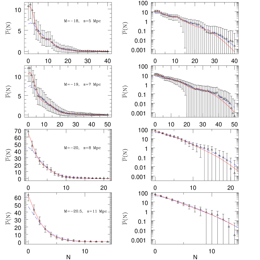
Figure 10:

Figure 11:

Figure 12:

Figure 13:

Figure 14:

Figure 15:

References

- (1) Balian, R., & Schaeffer R. 1989, A&A 220, 1
- (2) Benoist, C., Maurogordato, S., da Costa, L.N., Cappi, A., & Schaeffer, R. 1996, ApJ, 472, 452 (paper i)
- (3) Bernardeau, F., & Schaeffer, R. 1992, A&A, 255, 1
- (4) Bernardeau, F., & Schaeffer, R. 1996, in preparation
- (5) Bonometto, S.A., Borgani, S., Ghigna, S., Klypin, A., & Primack, J.R. 1995, MNRAS, 273, 101
- (6) Bouchet, F.R., & Hernquist, L. 1992, ApJ, 400, 25
- (7) Bouchet, F.R., Davis M., & Strauss M. 1992, in The Distribution of Matter in the Universe, IInd DAEC meeting, Mamon G.A. & Gerbal D. eds., Observatoire de Paris-Meudon, p.287
- (8) Bouchet, F.R., Strauss M.A., Davis M., Fisher K.B., Yahil A., & Huchra, J.P. 1993, ApJ, 417, 36
- (9) Cappi, A., & Maurogordato, S. 1995, ApJ, 438, 507
- (10) Cappi, A., da Costa, L.N., Benoist, C., & Maurogordato, S. 1998, AJ, in press
- (11) Carruthers, P., & Minh, D.V. 1983, Phys. Letters, 131B, 116
- (12) Coles, P., & Jones, B. 1991, MNRAS, 248, 1
- (13) da Costa, L.N., Geller, M., Pellegrini, P., Latham, D., Fairall, A., Marzke, R., Willmer, C., Huchra, J.P., Calderon, J.H. , Ramella M., & Kurtz, M.J. 1994, ApJ, 424, L1
- (14) da Costa, L.N. et al. 1998, AJ, in press (astro-ph/9804064)
- (15) Colombi, S., Bouchet, F.R., & Schaeffer, R. 1994, A&A, 281, 301 (CBS1)
- (16) Colombi, S., Bouchet, F.R., & Schaeffer, R. 1995, ApJS, 96, 401 (CBS2)
- (17) Efstathiou, G., & Jedrezejewski, R.I. 1984, Adv. Space Res., 3, No. 10-12, 379
- (18) Efstathiou, G., Ellis, R.S., & Peterson, B.A. 1988, MNRAS, 232, 43
- (19) Fry, J.N., & Seldner, M. 1982, ApJ, 259, 474
- (20) Fry, J.N. 1984a, ApJ, 277, L5
- (21) Fry, J.N. 1984b, ApJ, 279, 499
- (22) Fry, J.N. 1985, ApJ, 289, 10
- (23) Fry, J.N. & Gaztañaga, E., 1993, ApJ, 413, 447 (FG93)
- (24) Fry, J.N. & Gaztañaga, E., 1994, ApJ, 425, 1
- (25) Gaztañaga, E. 1992, ApJ, 398, L17
- (26) Gaztañaga, E. 1994, MNRAS, 268, 913
- (27) Gaztañaga, E. & Frieman, J.A. 1994, ApJ, 437, L13
- (28) Gaztañaga, E., Croft, R.A.C., & Dalton, G.B. 1995, MNRAS, 276, 336
- (29) Ghigna, S., Borgani, S., Tucci, M., Bonometto, S.A., Klypin, A., & Primack, J.P., 1997, ApJ, 479, 580
- (30) Giovanelli, R. & Haynes, M. P., 1989, AJ, 97, 633
- (31) Groth, E.J., & Peebles, P.J.E. 1977, ApJ, 217, 385
- (32) Hivon, E., Bouchet, F.R., Colombi, S., & Juszkiewicz, R. 1995, A&A, 298, 643
- (33) Huchra et al. 1997, preprint
- (34) Itoh, M., Inagaki, S., & Saslaw, W.C. 1993, ApJ, 403, 476
- (35) Juszkiewicz, R., Bouchet, F.R., & Colombi, S. 1993, ApJ, 412, L9
- (36) Juszkiewicz, R., Weinberg, D.H., Amsterdamski, P., Chodorowski, M., & Bouchet, F.R. 1995, ApJ, 442, 39
- (37) Kendal, M. & Stuart, A. 1991, Advanced theory of statistics, E. Arnold.
- (38) Kim, R.S. & Strauss, M.A. 1998, ApJ, 493, 39
- (39) Lahav, O., Itoh, M., Inagaki, S., & Suto, Y. 1993, ApJ, 402, 387
- (40) Matsubara, T., & Suto, Y. 1994, ApJ, 420, 497
- (41) Meiksin, A., Szapudi, I., & Szalay, A.S. 1992, 394, 87
- (42) Mo, H.J., & White, S.D.M. 1996, MNRAS, 282, 347
- (43) Mo, H.J., Jing, Y.P., & White, S.D.M. 1996, preprint (MJW)
- (44) Peebles P.J.E. 1980, The Large Scale Structure of the Universe, Princeton University Press, N.Y.
- (45) Plionis, M., & Valdarnini, R. 1995, MNRAS, 272, 869
- (46) Schaeffer, R. 1984, A&A, 134, L15
- (47) Schaeffer, R. 1985, A&A, 144, L1
- (48) Saslaw, W.C. & Hamilton, A.J.S. 1984, ApJ, 276, 13
- (49) Saslaw, W.C., Chitre, S.M., Itoh, M., & Inagaki, S. 1990, ApJ, 365, 419
- (50) Sheth, R.K., Mo, H.J., & Saslaw, W.C. 1994, ApJ, 427, 562
- (51) Willmer, C., da Costa, L.N., & Pellegrini, 1998, AJ, 115, 869
- (52) Yahil, A., Tammann, G.A., & Sandage, A. 1977, ApJ, 217, 903