A classical approach to faint extragalactic source extraction from ISOCAM deep surveys

Abstract

We have developed a general data reduction technique for ISOCAM data coming from various deep surveys of faint galaxies. In order to reach the fundamental limits of the camera (due to the background photon noise and the readout noise), we have devised several steps in the reduction processes that transform the raw data to a sky map which is then used for point source and sligthly extended source extraction. The main difficulties with ISOCAM data are the long-term glitches and transient effects which can lead to false source detections or large photometric inaccuracies. In many instances, redundancy is the only way towards clear source count statistics. A sky pixel must have been “seen” by many different CAM pixels. Our method is based on least-squares fits to temporal data streams in order to remove the various instrumental effects. Projection onto the sky of the result of a “triple–beam method” (ON -(OFF1 + OFF2)/2) obtained from the signal of a given pixel during three consecutive raster positions leads to the removal of the low frequency noise. This is the classical approach when dealing with faint sources on top of a high background. We show illustrative examples of our present scheme by using data taken from the publicly available Hubble Deep Field ISOCAM survey in order to demonstrate its characteristics.

More than thirty sources down to the 60 (resp. 100) $\,\mu{\rm Jy}\,$level are clearly detected above 4 $\sigma$ at wavelengths of 7 (resp. 15) $\,\mu{\rm m}\,$, the vast majority at 15 $\,\mu{\rm m}\,$. A large fraction of these sources can be identified with visible objects of median magnitude 22 and K–band magnitude of 17.5 and redshifts between 0.5 and 1 (when available). A few very red objects could be at larger redshifts.

1 Introduction

After the first ISOCAM results on relatively strong sources (ISO A&A 1996, 315, special issue) it has become clear that the Camera on ISO could achieve more sensitive observations by integrating longer, particularly on “empty” high galactic latitude fields. Already sources with fluxes larger than the mJy level can routinely be observed which are 1000 times fainter than previous IRAS 12$\,\mu{\rm m}\,$ surveys and with a resolution which is 10 times higher. Reduction of the data requires that effort has to be spent on dealing with CAM peculiarities which show up at these levels. The now “old” mid-infrared detectors on ISO, which were designed ten years ago, suffer from long–term memory effects that have to be dealt with, before the noise can be integrated down. We will show that this is possible because the camera is ultimately highly linear when stabilised, and the so–called transient effects are highly reproducible under the same conditions, and because the zodiacal background, which dominates the high galactic latitude sky in the long wavelength (LW) channel, appears to be smooth on the 10 arcsecond scale. As many important projects with ISOCAM (several hundred hours from both guaranteed and open time proposals) aim at looking for faint extragalactic objects, it is worth developing and demonstrating reliable, independent data reduction techniques. Our approach is complementary to the method presented by Starck et al. (1998) and Aussel et al. (1997, 1998). We will here present how the raw data are processed to remove the main instrumental effects (Sect. 2), and how the triple beam–switch reduced data are projected onto the sky and sources are extracted from the resulting sky map (Sect. 3). At each step, for illustrative purposes, we take examples from the HDF public domain ISOCAM data (Rowan–Robinson et al. 1997). All of our algorithms were developed on Dec-Alpha stations using specific routines written in the IDL language. We then apply the whole ISOCAM data reduction method to the HDF specific case and give a list of the faintest mid-infrared sources that have been observed to date (Sect. 4). Finally we briefly discuss the advantages and drawbacks of this method and the various ways it could be improved.

2 The ISOCAM data processing

2.1 Reading the raw data

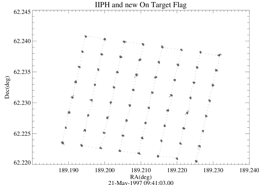
Figure 1: ISO pointing history taken from IIPH22701702. Consecutive points are separated in time by half a second. The positions in RA and Dec (2000) are smoothed with a 2 second temporal kernel. One must mask out readouts which were taken when during some part of them, ISO was moving.

Raw telemetry from ISO is converted into different formats and delivered by ESA to the community. We chose to start from SPD FITS files. This means that the pair of reset and end-of-integration images are already subtracted. The CISP (almost raw) data are read into a dataset which contains, along with the data cube (of size 32 by 32 by the total number of readouts), a header describing the context of the observations, and various trend parameter arrays (CAM wheel positions, various ISO time definitions) which are or are not synchronised with the images. An important trend parameter set is the pointing information from the ISO satellite which is read from the appropriate IIPH (ISO Instrument Pointing History) FITS file and appended to the raw dataset. The equatorial right ascension (RA) and declination (Dec) coordinates (in the J2000 system) pointed to by the centre of the camera suffer from some noise (not corresponding to a real ISO jitter). These are smoothed with a running kernel with a FWHM of 2 arcseconds which give a relative pointing accuracy better than one arcsecond (Fig. 1). The pointing data are synchronised to the dataset cube of images by using the UTK time that is common to CISP and IIPH files. Data are usually taken in a raster mode where a regular grid of pointings on the sky is done successively. Care should be taken not to use the on-target flag delivered in the CISP file. This flag is set to one when the acquired pointing is within 10 arcsecond of the required raster pointing. This flag is obviously too loose if one uses the 6 or, even worse, the 3 arcsecond lens. A 2 arcsecond radius of pointing tolerance is used here for our own criterion.

At this stage the data in the ISOCAM internal units of ADU (Analog–to–Digital Units) are converted to ADUG units by simply dividing by the gain (equal to $2^{\tt F2\_ADC\_GAIN}$). A library dark image is then subtracted, the accuracy of which is not relevant in the following. In the next three sub–sections we consider each pixel as individual detectors and analyse their temporal behaviour without regard to their neighbours. A mask cube of the same size as the data cube is used in parallel to flag the data which are affected by various damaging effects.

2.2 Removing particle hits

2.2.1 Fast glitch correction

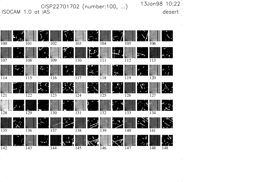
Figure 2: A sample of elementary successive images with the ISO 32 by 32 pixel LW camera taken from the CISP22701702 data set, number 100 to 148 (starting at 0). After each image, a mask deduced from the short deglitching algorithm shows the numerous impacts of cosmic rays. (Configuration of the camera is LW3 filter, LGe6 lens, 36 camtu (=5 seconds) of elementary integration time.)

At first glance (Fig. 2), any readout obtained with ISOCAM not containing strong sources (fluxes larger typically than about 10 mJy in the broad filters) clearly shows the flat field response by the pixels to the zodiacal background. Ultimately, it is the accuracy to which one knows this flat–field that allows identification of faint sources (see Sect. 2.4).

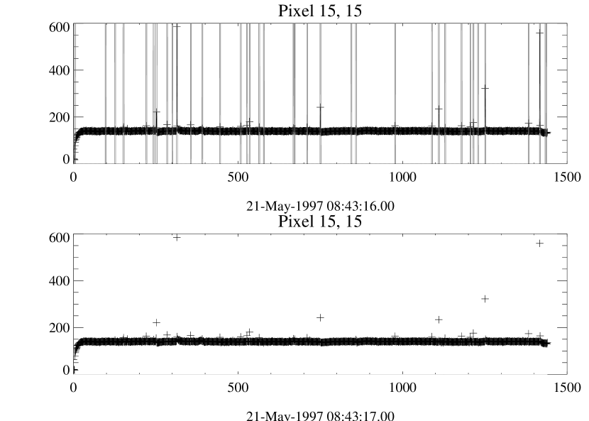
Figure 3: Temporal evolution of the raw signal (in ADUG i.e. Analog–to–Digital Units divided by the gain) from camera pixel 15, 15 (starting at 0, 0) taken in CISP22701702 (abscissa is in readout number starting at 0 for the first readout of the dataset). Upper panel – A mask of readouts affected by fast glitches as deduced by the algorithm described in the text (dotted vertical lines). Lower panel – the raw data

Detectable signals from some pixels which are often aligned in strings result from hits by cosmic ray particles. Most of the affected pixels recover at the next or second next readout. These are mainly due to primary and secondary electron energy deposition onto the array.

The affected pixels are found by an algorithm working on the temporal behaviour of each pixel. Readouts of one pixel which deviate from the running (14 readouts) median by more than a threshold value and tend to recover to the normal level by at least 10 percent of the maximum step after one or two readouts are simply masked for two readouts and excluded from further signal extraction. The threshold value is set by a number (typically 3) times a running window (14 readouts) standard deviation of the pixel signal, where the most deviant values have been excluded from the rms computation. This algorithm was tested in various cases, and in particular against false glitch detection around the typical signal of a moderately strong source. Figure 3 shows an example of the temporal behaviour of one CAM pixel as a function of readout number.

The number of glitches, or more precisely, the number of readouts which are affected by the masking process, is typically 9 per second over the entire array of 992 alive pixels: e.g. during an integration time of $t_{int}$ = 36 camtu = 5 seconds, at any time 45 pixels cannot be used for measurement. This number varies by at least 15 percent apparently depending on the satellite orbiting position. Accumulated glitches cause a noticeable increase in the noise or an unreliable measurement. We thus decided to mask an isolated “good” readout value if it is between two successive glitches. The energy deposition has a continuum distribution that goes down to the intrisic noise level of the camera. For the method presented here, any undetected faint glitch contributes to increase the statistical noise and to modify slightly the signal.

2.2.2 Slow glitch correction

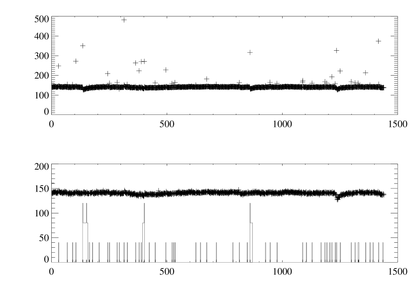
Figure 4: Temporal evolution of the raw signal (in ADUG) from camera pixel 16, 15 (starting at 0, 0) taken in CISP22701702 (abscissa is in readout number starting at 0 for the first readout of the dataset). a – Raw signal (except for the removal of the first camera overall transient which can be seen in the previous figure) b – The signal after the removal of slow glitches and the adapted mask (40 is for a fast glitch, see Sect. 2.2.1, and 80 for a slow glitch,see Sect. 2.2.1): a non vanishing mask corresponds to a value which will not be used for further processing, masked values are not shown. The dip near readout 1250 is not corrected at this stage.

These are the most difficult to deal with. They are the main limitation in detecting weak point-like or extended sources and are thought to be due to ion impacts. These impacts affect the response of the hit pixels with a long memory tail. Slow glitches are of three types: 1) Positive decay of short time constant (5-20 seconds), 2) Negative decay of long time constant (up to 300 seconds) 3) A combination. It is possible that positive decay glitches are due to an ionisation or energy deposition which does not saturate the detector. Negative ones may have started with saturation (which is not apparent in the readout value) and hence cause memory effects, an upward transient of a type not very different from the usual CAM transient starting from a low flux.

Figure 4a shows the effect of slow glitches. In Fig. 4b the corrected signal is shown along with the used mask. To detect slow glitches we correlate a running template of a typical glitch along the temporal signal $D_{t}$ of a given pixel. A maximum in the correlation indicates a potential glitch at say $t_{0}$. This is then analysed with a least-square method in order to find the best decay time constant: one minimises the $L_{a}$ quantity defined by

$$L_{a}^{2} = \Sigma_{t}w_{t}(D_{t}-M_{t})^{2}{\,\rm with\,}$$ (1)

$$M_{t} = A+Bt+H(t-t_{0})G\exp{\big{(}-{(t-t_{0})\over\tau}\big{)}},$$ (2)

where $D_{t}$ is the raw temporal data signal of a pixel, $w_{t}$ the weight (0 or 1, defined by the previous masking of fast glitches), $M_{t}$ the glitch model to fit, and $t_{0}$ is given. Hence, the variables $A$, $B$, $G$, and $\tau$ are found ($H$ is the Heaviside jump function).

If the fit is satisfactory, we subtract the exponential part of the fit up to the end of the temporal signal. To assess whether the fit is satisfactory or not, we also calculate the least-square $L_{b}$ corresponding to a linear baseline without the exponential part. We found that, a potential glitch can be taken as valid if $L_{a}\leq L_{b}/2$. Most of the time, the glitch beginning at time $t_{0}$ corresponds to a previously detected fast glitch.

Type 1 glitches can be removed with the previous method but, sometimes, the same method also removes real source signals (for example, if there is a downward transient when a pixel leaves a source). We thus leave Type 1 glitches to be removed later in the method. Type 3 glitches are not dealt with at the moment. The running template to detect a glitch and find its starting time $t_{0}$ is a simple exponential with successive time constants of 15, 30, and 60 readouts for negative glitches (Type 2 glitches). After a glitch is found at a significant level, and the exponential tail is corrected everywhere after $t_{0}$, we mask (i.e. we will not further use) the readouts for times between $t_{0}$ and the time $t_{1}$ where the amplitude of the exponential correction is above twice the pixel noise per readout. An example can be found in Fig. 4.

Typically one new slow negative glitch appears somewhere on the camera every 1.2 second. Its intensity ($G$) varies from 5 to 20 ADUG. The time constant varies from 20 to 200 seconds (45 is typical). Positive glitches are 10 times rarer.

2.3 Removing transient effects: a simple correction technique

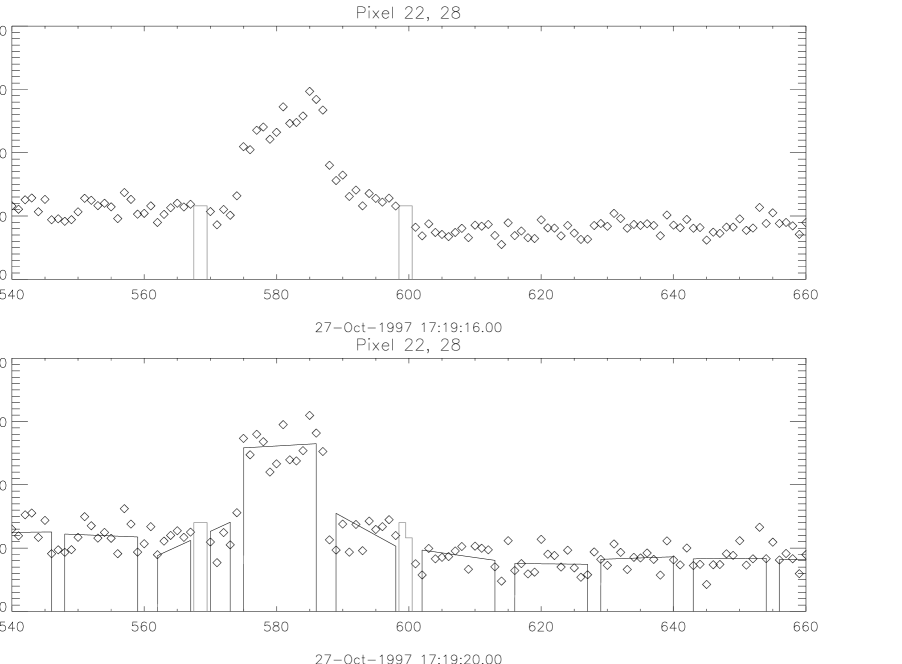
Figure 5: a – The transient phenomenon of ISOCAM is illustrated on a relatively strong source taken from ISOCAM guaranteed time deep surveys. The signal $D_{t}$ is shown in ADUG as a function of readout number. Eight ISO raster positions are within the plot. At readout 575, just after ISO moved, the pixel (22, 28) instantaneously responds to the illumination added by a (rather strong) source on top of the zodiacal background, but it also has a long lagged response (mask is in dotted line). After ISO moved to the next raster position, one can still see the memory effect of the source. b – The recovered illumination history $I_{t}$ of the same pixel after inversion of the transient model (Eq. 4). The solid line is the result of the triple–beam switch fitting (Eq. 6, only the central part of the three–leg best fit of each raster position is shown for simplicity). The fit is done on valid readouts within each raster position, as delimited by the vertical lines. No sources in the HDF can be seen as vividly as here because they are much fainter.

ISOCAM, like many other infrared detectors, suffers a lag in its response to illumination. Fortunately, the LW detector has a significant instantaneous response $r\simeq 0.60$ i.e. a jump in brightness is seen at once by the pixel at the level of 60% of the step relative to its stabilised asymptotic value. The remainder of the signal is obtained after a delay which is inversely proportional to the flux. In a first approximation, Abergel et al. (1996) have modelled this phenomenon with:

$$D_{t}=rI_{t}+(1-r)\int^{t}_{-\infty}dt^{\prime}k_{t^{\prime}}I_{t^{\prime}}e^{-k_{t^{\prime}}(t-t^{\prime})}{\,\rm and\,}$$ (3)

$$k_{t^{\prime}}=\alpha I_{t^{\prime}}\simeq\alpha D_{t^{\prime}},$$ (4)

where the measured signal $D_{t}$ at time $t$ is a function of the illumination $I_{t^{\prime}}$ at previous times, and

$$\alpha=1200\rm\,ADUG^{-1}readout^{-1},$$ (5)

where an ADUG is the CAM analog to digital unit normalised by the used gain. The approximation for $k$ in eq. 4 makes it possible to invert the triangular temporal matrix. The inversion algorithm is independent of the position of the satellite and makes no a priori assumption as to the temporal evolution of the pixel intensity history. It also preserves the volume of the data cube. An example of a relatively strong source is shown in Fig. 5a. The inversion (getting $I$ from $D$) yields the result shown in Fig. 5b. The inversion apparently enhances the high frequency noise of the pixel but the signal to noise ratio stays constant because the overall ISOCAM calibration must be updated after the transient correction has been applied.

The correction helps in improving the calibration accuracy because it gives the proper stabilised value that can be directly tied to a response measured on bright stabilised stellar standards. It also removes ghosts of sources which otherwise can still be seen after the pixel has been pointed away from the source to its next raster position (see Fig. 5a). We believe this correction works best for faint sources, the main objective of the present study. The correction is not yet perfect and further understanding of the camera lag behaviour will certainly provide improvements in the final calibration.

2.4 Removing long term drifts: the triple beam-switch method

The data cube should now contain a signal in the unmasked areas, which is almost constant for a given raster position and a given pixel. At this stage, we remove most of the slow positive glitches for a given pixel

1. by computing the standard deviation found inside each configuration (i.e. one raster position) and by taking the median average of this deviation for all configurations.

2. by masking a readout if it deviates by more than 4 times this typical noise from the median level of its configuration

The value of 4 was found by trial and error.

We are then left with a data cube where all or almost all “bad” pixels have been masked and therefore are not used further. As there is still some low-frequency noise for each pixel, we do not feel ready yet to project the total power value of each pixel on the sky but instead we prefer comparing the values during a raster position to the values in the two adjacent raster positions seen by the same CAM pixel. This is the classical approach for dealing with low-frequency noise. It is usually adopted when the background is much stronger than the sources: a regime which has long been the case in infrared astronomy and which is now appearing even in optical astronomy. This approach has been pioneered by e.g. Papoular (1983).

This is done with the following least-square method which is independently applied to each pixel (where $i$ is the readout number proportional to the time $t_{i}$ which runs along the 3 current raster positions centered at the mid time), by minimising:

$$Ls=\sum_{i}w_{i}(D_{i}-(a+bt_{i}+up_{i}))^{2},$$ (6)

where $w_{i}$ is 1 for valid readouts and 0 for masked readouts or readouts which do not belong to the three current raster positions e.g. when ISO was moving (see Sect. 2.1). $D_{i}$ is the pixel signal at readout $i$. $p_{i}$ is the template of a source, typically a square pattern (0…0, 1,…,1,0…0) template, where the ones are set for the central raster position. The best $a$, $b$, and $u$ are therefore obtained from the minimisation of $Ls$. The method gives an estimate of the noise on the $a_{b}$, $b_{b}$, and $u_{b}$ parameters by assuming that roughly $\sigma^{2}=Ls_{b}/(\sum_{i}w_{i}-3)$ (because 3 parameters are fitted) so that the noise per readout is $\sigma$ and $Ls_{b}$ is obtained from formula 6. The value of $u_{b}$ (simplified to $u$ in the following) corresponds to the best estimate of the average signal for each pixel and raster position. The associated noise $\sigma_{u}$ and $Ls_{b}$ are recorded for a given pixel at a given raster position. The uncertainty on the pixel signal $\sigma_{u}$ is itself quite noisy for a given raster position so in fact we replace it by the median of all $\sigma_{u}$ found during the raster for that particular pixel (the quality of the fit $Ls_{b}$ is modified accordingly). As a complementary and very effective glitch removal, we mask the signal of a given raster position if its $Ls_{b}$ deviates by more than a factor 2 from the pixel median value across all rasters or if the number of points used for the fit is less than a factor of 0.6 times the median value. No detection of a point source is made at this stage. Hence, the data cube is reduced to a few values per raster position and per pixel of the camera. For the first and last positions of the raster, we use a 2-beam differencing scheme similar to the 3-beam scheme presented except that no slope $b$ can be found. We checked, a posteriori, that the distribution of all the values of the signal $u$ divided by their respective noise $\sigma_{u}$ precisely follows a reduced Gaussian (actually we slightly overestimate the noise by up to 15 percent), except for the few pixels affected by sources. This is strong evidence that white noise dominates the output of this algorithm.

Note that the standard raster averaging method followed by ON-(OFF1+OFF2)/2 differencing scheme would have worked in most situations except that here the noise can be estimated independently, the least square statistics can be used as an effective glitch removal, and, in the case of several randomly placed masked values the baseline removal is better defined. Note also that the noise of the triple beam-switch method is $\sqrt{3/2}$ worse than for an absolute measurement (in case the flat field were perfectly known). But the low-frequency noise is here largely suppressed which overbalances the loss of sensitivity, which in principle costs an integration time longer by 50 percent on target.

3 Projection onto the sky and extraction of sources

3.1 Projection onto the sky

The reduced cube ($u$) can now be flat fielded (FF). Notice that at this stage the FF only applies to values which are close to zero and that the precision for this FF is not critical. Actually, the method outlined above provides a natural FF for the data, namely the median of the fitted background (as given by the term $a_{b}+b_{b}t_{ic}$ applied to the central time of each raster) along all raster positions. By convention (ISOCAM Consortium), the FF is normalised to one in the central 144 pixels of the camera. A dark removal is required only for this FF (see Sect. 2.1); thus, no precise dark is really required in the entire reduction procedure. The dark level, even if it slowly fluctuates, is removed by the beam-switch technique. The FF is applied to both the data and the noise cubes ($u$ and $\sigma_{u}$).

The data are then projected onto a sky map (RA, DEC: epoch 2000) with a closest pixel method and fine sampled pixels (we use 1.5 arcsecond pixels on the sky for the 6 arcsecond lens, an integer multiple so that the method preserves fluxes). A projection of each CAM raster plane is done by using the raster central position (RA, DEC) and roll angle (ROLL) from the IIPH raster averaged values. Corrections are done for the slightly distorted camera field-of-view. A gnomonic projection type is used as with IRAS. Usually a pixel on the sky has been measured by different pixels of the camera. We use an optimised averaging of these different measurements with a $1/\sigma_{u}^{2}$ weighting. A sky noise map is then also deduced from this optimised averaging. A scaling is applied to this sky noise map in order to take into account the correlation of noise in the oversampled sky pixel map across each camera pixel extension.

3.2 Detection of point-sources and photometry

So far, no bias has been introduced against positive or negative (if any!) flux sources, extended or point sources, except for sources more extended than the raster step for which the beam-switching reduction technique is not appropriate. A side effect of the method is to leave negative sources of half flux near any positive source along the raster direction at a raster step distance. Indeed, the fitting algorithm of Sect. 2.4 will find a negative signal of minus half the central value, on the raster positions that are adjacent to a strong positive signal position. A more sophisticated algorithm would be required near the confusion limit.

Point sources are searched for with a top-hat 2 dimensional wavelet. A 2D Gaussian of fixed width is then fitted (with a simple least square method) around the candidate position on the sky map in intensity and position along with a flat background (see a discussion by Irwin, 1985). For the HDF, we have used an 8 arcsecond (resp. 4) FWHM Gaussian for the 6 (resp. 3) arcsecond lens. This routine was implemented to deal with both the undefined values, which are scattered around because of the masking applied to the data cube and its projection onto the sky, and the non-uniform noise maps (affecting the weight of each pixel in the fit in the optimal $1/\sigma^{2}$ way). The final flux of a source is given as the 2D Gaussian integrated ADUG. The error on the flux is deduced from the error sky map that was produced in the previous section. Fluxes in $\,\mu{\rm Jy}\,$are obtained by dividing fluxes by the integration time per readout (ADUG/$t_{int}$) and the conversion table in the ISOCAM cookbook multiplied with an efficiency factor which happens to be unity (the temporary $\simeq 0.8$ absolute calibration for stabilised point sources quoted by Cesarsky et al. (1996) has since been revised upward). The fluxes are then scaled by a number 1.83 (resp. 1.87) for LW2 (resp. LW3) that was determined by simulating the ISO PSF, its modulation by the triple–beam method (that produces negative half-flux ghost sources on the sides) and the Gaussian fit with a fixed FWHM, in order to recover the whole camera efficiency. Fluxes are given at the nominal wavelength of 6.75 (resp. 15) $\,\mu{\rm m}\,$with an assumed spectral dependence $F_{\nu}\propto\nu^{-1}$ (IRAS convention). After the strongest source is found and its Gaussian flux removed from the map, one repeats the Gaussian fitting procedure to find the next source. It is then removed and one iterates the method in order to produce a catalog of candidate sources with position, flux and errors.

3.3 Detection of slightly extended sources

The Gaussian fitting allows going to the faintest level of point source detection but misses part of the flux if the source is extended. We can also compute a fixed aperture photometric flux in order to check for possible extensions with different apertures (although for the particular HDF ISOCAM data we have not done so because of the small raster steps). These fluxes are noisier but they allow a more appropriate measurement for extended sources. Geometric parameters can also be deduced following the methods of Jarvis & Tyson (1981) and Williams et al. (1996).

3.4 Reproducibility

The redundancy factor (the number of times a sky pixel was seen by different pixels on the camera) is a key factor in deciding the reliability of sources. So far we have kept as reliable candidates those sources which have been covered during at least two raster positions by unmasked camera pixels. Quality criteria on the photometric consistency can then be given to each point-source candidate. For this purpose, we can independently project three subrasters made out of every third raster values of the $u$ cube onto the sky. For each subraster, we measure the flux ($F_{1s}$, $F_{2s}$, $F_{3s}$) and flux uncertainty ($U_{1s}$, $U_{2s}$, $U_{3s}$) of each source $s$ found in the total map (of flux $F_{ts}$ and noise $U_{ts}$) at the same position. We define the quality $Q1_{s}$ of a source as the highest ranking condition that it meets, according to:

$$Q1_{s} =4{\rm\ if}\ |F_{is}-F_{ts}|\leq 2U_{is}$$ (7)

$$=3{\rm\ if}\ |F_{is}-F_{ts}|\leq 3U_{is}$$

$$=2{\rm\ if}\ |F_{is}-F_{ts}|\leq 4U_{is}$$

$$=1{\rm\ if}\ F_{is}\geq 3U_{is}{\rm\ and\ }F_{ts}\geq 5U_{ts}$$

$$=0{\rm\ otherwise,}$$

where the condition must hold for all the 3 subraster index $i$ (from 1 to 3). Clearly, the quality from 2 to 4 gives an increasing confidence in the source reliability. We added the level of 1 for strong signal-to-noise sources which can be otherwise dropped because the flux reproducibility (and not the statistical significance) is then more difficult to achieve: this source noise happens because of the ISO jitter, the errors in the projection process and the undersampling of the PSF. We define a secondary quality $Q2_{s}$ criterion for low redundancy surveys according to the same logic as Eq. 7 but keeping only the two flux values with the lowest noise out of the 3 subraster fluxes.

The reduction of several independent surveys of the same area (slightly shifted if possible) allows a control of systematics. The relative photometric accuracy is generally achieved at the ten percent level while the absolute photometric accuracy is not better than the thirty percent level (as deduced from weak calibrated stars and using the known linearity of the stabilised camera). It seems that stronger sources do not have better signal-to-noise (than say 30) because other errors (the source noise mentioned above is proportional to the signal) can occur. We found that sources in common in the different surveys agree well in position (say within a CAM pixel or two). At present, the comparison of various ISOCAM datasets with other surveys (in optical and radio) confirms the astrometric precision of 6 arcsecond radius at the $2\sigma$ level.

4 The HDF data analysis

Table 1: : HDF-2_LW2 list of significant sources at the $3\sigma$ level found in the raster with TDT no 22401501, corrected by -1.90, -1.80 arcseconds

Name		$\alpha$			$\delta$		F1	U1	S/N1	F2	U2	S/N2	F3	U3	S/N3	Ft	Ut	S/Nt	Q1	Q2
	hr	mn	sec	deg	’		$\mu$Jy	$\mu$Jy		$\mu$Jy	$\mu$Jy		$\mu$Jy	$\mu$Jy		$\mu$Jy	$\mu$Jy
HDF-2_LW2_1	12	36	46.4	62	14	3.4	91.	26.	3.6	32.	26.	1.2	82.	26.	3.1	69.	15.	4.6	4	4
HDF-2_LW2_2	12	36	48.3	62	14	26.4	50.	29.	1.8	100.	27.	3.6	133.	27.	5.0	96.	16.	6.0	4	4
HDF-2_LW2_3	12	36	49.7	62	13	46.9	11.	26.	0.4	79.	27.	3.0	59.	26.	2.2	48.	15.	3.2	4	4
HDF-2_LW2_4	12	36	52.3	62	13	14.9	25.	27.	0.9	41.	27.	1.5	82.	26.	3.1	49.	15.	3.2	4	4

Table 2: HDF-4_LW2 list of significant sources at the $3\sigma$ level found in the raster with TDT no 22401305, corrected by 0, 0 arcseconds

Name		$\alpha$			$\delta$		F1	U1	S/N1	F2	U2	S/N2	F3	U3	S/N3	Ft	Ut	S/Nt	Q1	Q2
	hr	mn	sec	deg	’		$\mu$Jy	$\mu$Jy		$\mu$Jy	$\mu$Jy		$\mu$Jy	$\mu$Jy		$\mu$Jy	$\mu$Jy
HDF-4_LW2_1	12	36	36.8	62	12	10.8	62.	44.	1.4	152.	40.	3.8	33.	43.	0.8	85.	24.	3.5	4	4
HDF-4_LW2_2	12	36	37.3	62	11	30.6	330.	92.	3.6	177.	77.	2.3	43.	75.	0.6	172.	46.	3.7	4	4

Table 3: : HDF-2_LW3 list of significant sources at the $3\sigma$ level found in the raster with TDT no 22701702, corrected by -1.20, -4.10 arcseconds

Name		$\alpha$			$\delta$		F1	U1	S/N1	F2	U2	S/N2	F3	U3	S/N3	Ft	Ut	S/Nt	Q1	Q2
	hr	mn	sec	deg	’		$\mu$Jy	$\mu$Jy		$\mu$Jy	$\mu$Jy		$\mu$Jy	$\mu$Jy		$\mu$Jy	$\mu$Jy
HDF-2_LW3_1	12	36	34.2	62	12	30.6	337.	147.	2.3	209.	133.	1.6	442.	154.	2.9	322.	83.	3.9	4	4
HDF-2_LW3_2	12	36	36.2	62	13	39.0	182.	75.	2.4	288.	74.	3.9	289.	73.	4.0	254.	43.	6.0	4	4
HDF-2_LW3_3	12	36	39.2	62	14	23.4	53.	67.	0.8	144.	70.	2.1	183.	75.	2.4	123.	41.	3.0	4	4
HDF-2_LW3_4	12	36	39.6	62	12	42.9	217.	65.	3.4	231.	65.	3.6	403.	65.	6.2	284.	37.	7.6	4	4
HDF-2_LW3_5	12	36	43.9	62	12	44.5	161.	55.	3.0	138.	56.	2.5	264.	56.	4.7	188.	32.	5.8	4	4
HDF-2_LW3_6	12	36	46.3	62	14	3.9	153.	55.	2.8	49.	54.	0.9	166.	54.	3.1	122.	31.	3.9	4	4
HDF-2_LW3_7	12	36	46.4	62	15	30.2	81.	80.	1.0	383.	73.	5.2	291.	74.	3.9	256.	43.	5.9	3	4
HDF-2_LW3_8	12	36	46.5	62	14	48.3	87.	54.	1.6	114.	53.	2.2	170.	58.	2.9	122.	32.	3.9	4	4
HDF-2_LW3_9	12	36	48.4	62	14	26.4	308.	53.	5.8	241.	54.	4.4	219.	55.	4.0	256.	31.	8.2	4	4
HDF-2_LW3_10	12	36	49.3	62	14	5.5	52.	56.	0.9	167.	57.	2.9	73.	54.	1.3	98.	32.	3.0	4	4
HDF-2_LW3_11	12	36	49.7	62	13	13.0	259.	53.	4.9	260.	51.	5.1	243.	52.	4.7	254.	30.	8.5	4	4
HDF-2_LW3_12	12	36	51.1	62	13	17.0	174.	53.	3.3	67.	51.	1.3	44.	54.	0.8	95.	30.	3.1	4	4
HDF-2_LW3_13	12	36	51.8	62	13	54.1	142.	54.	2.6	238.	53.	4.5	112.	54.	2.1	165.	31.	5.3	4	4
HDF-2_LW3_14	12	36	53.9	62	12	53.6	109.	52.	2.1	183.	53.	3.4	163.	55.	2.9	151.	31.	4.9	4	4
HDF-2_LW3_15	12	36	57.9	62	14	56.5	91.	60.	1.5	147.	66.	2.2	266.	62.	4.3	165.	36.	4.6	4	4
HDF-2_LW3_16	12	36	60.0	62	14	53.2	276.	62.	4.5	352.	65.	5.4	268.	65.	4.2	299.	37.	8.1	4	4
HDF-2_LW3_17	12	37	2.5	62	14	4.3	196.	61.	3.2	188.	67.	2.8	187.	63.	3.0	190.	37.	5.2	4	4
HDF-2_LW3_18	12	37	4.9	62	14	31.2	115.	76.	1.5	181.	79.	2.3	120.	78.	1.5	137.	45.	3.1	4	4

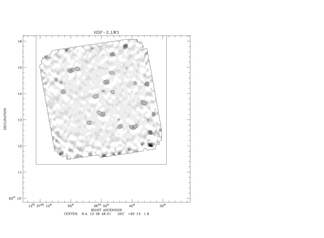
Figure 6: LW3 grey scale map of the HDF-2 raster. The contour is at about the 3 $\sigma$ level. Black corresponds to about 300$\,\mu{\rm Jy}\,$per beam, white to 0. Following maps are done on the same scale.

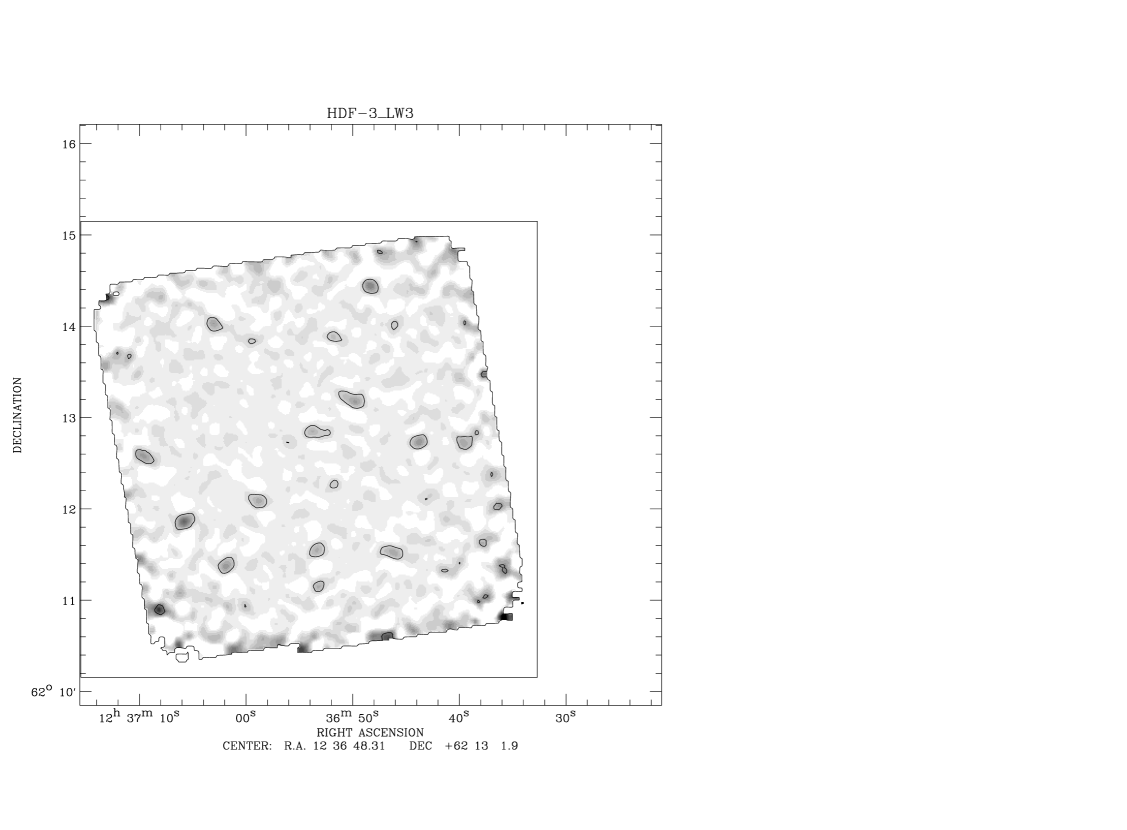
Figure 7: HDF LW3 grey scale map of the HDF-3 raster. Contour and greyscale are identical to the previous figure.

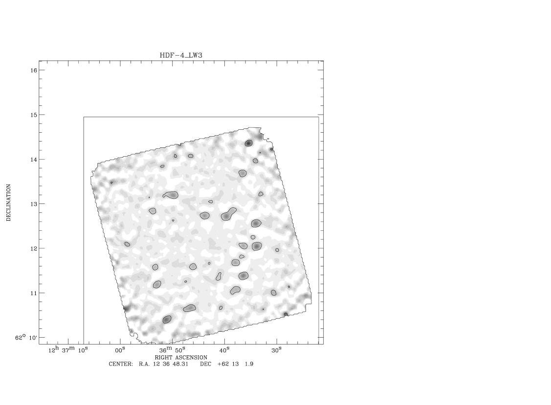
Figure 8: HDF LW3 grey scale map of the HDF-4 raster. Contour and greyscale are identical to the previous figure.

The data in the public domain on the Hubble Deep Field in the LW2 (6.7$\,\mu{\rm m}\,$) and LW3 (15$\,\mu{\rm m}\,$) ISOCAM-LW bands are analysed here with the method outlined above. Early results are given by Rowan–Robinson et al. (1997). The data were taken in three rasters for each wavelength centered on the optical centre of the Hubble Space Telescope WFPC quadrants number 2, 3 and 4. The 3 arcsecond lens was used for LW2 and the 6 arcsecond lens for LW3. The LW3 rasters are therefore largely overlapping. Adjacent raster positions are separated by resp. 5 and 9 arcseconds, roughly a pixel and a half apart. The resulting triple beam-switch method that we apply may miss a fraction of the flux (although we have tried to evaluate it in Sect. 3.2), in that particular case, especially if there are extended objects. Each raster is made of 8 by 8 positions aligned with the camera axes (see Fig. 1). Each LW2 (resp. LW3) raster position is made of resp. 9 to 10 (19 to 20) readouts of 72 (resp. 36) CAMTU (10 and 5 s resp.) integration times. Tables 1 and  2 and Tables 3, 4, & 5 give the details of potential sources with a quality different from 0 (either $Q1$ or $Q2$) for each ISO raster (no significant source was found with LW2 in the third HDF quadrant). The source positions for each raster are corrected by an absolute astrometric offset. This offset was determined from the sources which are detected in several rasters, the optical identification for the primary astrometric corrector is a 19.5 magnitude object (with a redshift of 0.139, Cowie et al. 1998) situated at (J2000) RA= 12 36 48.33 and Dec= 62 14 26.4 at the upper part of the HDF, which is detected at both wavelengths. Note that we could not coadd LW2 rasters (they do not overlap much anyway) because of the lack of common sources or well identified sources. Figure 6, 7 and 8 show the 3 independent LW3 rasters with intensity in greyscale and 3 $\sigma$ contours. One can notice at once the large consistency between the 3 independent datasets in the overlapping area. Figure 9 shows an f814 HST image of the HDF (Williams et al. 1996) superposed by a 3 $\sigma$ contour of ISOCAM after shifting and optimally coadding the three individual LW3 rasters. Table 6 presents the final list of objects detected in the LW3 coadded map. Figure 10 shows a K-band IRIM image of the HDF (Dickinson et al. 1997) superposed by a 3 $\sigma$ contour of the same ISOCAM LW3 total map. It is clear that the sources in the final catalog (table 6) that are not in one or two of the raster tables (3, 4, & 5) are simply outside or at the edge of the corresponding observed area.

Table 4: : HDF-3_LW3 list of significant sources at the $3\sigma$ level found in the raster with TDT no 22701604, corrected by -1.20, -7.10 arcseconds

Name		$\alpha$			$\delta$		F1	U1	S/N1	F2	U2	S/N2	F3	U3	S/N3	Ft	Ut	S/Nt	Q1	Q2
	hr	mn	sec	deg	’		$\mu$Jy	$\mu$Jy		$\mu$Jy	$\mu$Jy		$\mu$Jy	$\mu$Jy		$\mu$Jy	$\mu$Jy
HDF-3_LW3_1	12	36	39.4	62	12	44.0	349.	83.	4.2	137.	81.	1.7	213.	83.	2.6	232.	47.	4.9	4	4
HDF-3_LW3_2	12	36	42.9	62	12	8.2	152.	56.	2.7	133.	59.	2.2	25.	60.	0.4	106.	34.	3.1	4	4
HDF-3_LW3_3	12	36	43.8	62	12	44.3	241.	56.	4.3	199.	59.	3.3	224.	60.	3.7	222.	34.	6.6	4	4
HDF-3_LW3_4	12	36	46.2	62	11	31.8	157.	63.	2.5	276.	59.	4.7	167.	60.	2.8	200.	35.	5.7	4	4
HDF-3_LW3_5	12	36	48.3	62	14	26.4	431.	81.	5.3	167.	77.	2.2	253.	83.	3.0	279.	46.	6.1	4	4
HDF-3_LW3_6	12	36	49.8	62	13	11.7	177.	53.	3.3	184.	54.	3.4	344.	53.	6.5	236.	31.	7.7	3	3
HDF-3_LW3_7	12	36	51.7	62	13	53.2	140.	57.	2.5	76.	60.	1.3	136.	57.	2.4	119.	33.	3.6	4	4
HDF-3_LW3_8	12	36	53.2	62	11	9.3	95.	79.	1.2	211.	75.	2.8	150.	76.	2.0	147.	45.	3.3	4	4
HDF-3_LW3_9	12	36	53.3	62	11	33.1	185.	62.	3.0	218.	57.	3.8	132.	56.	2.4	180.	34.	5.4	4	4
HDF-3_LW3_10	12	36	53.6	62	12	50.9	101.	53.	1.9	137.	55.	2.5	267.	56.	4.8	167.	32.	5.3	4	4
HDF-3_LW3_11	12	36	58.9	62	12	5.2	205.	52.	3.9	200.	55.	3.6	157.	53.	3.0	188.	31.	6.1	4	4
HDF-3_LW3_12	12	37	1.9	62	11	23.1	149.	73.	2.1	434.	75.	5.8	147.	66.	2.2	239.	41.	5.8	3	4
HDF-3_LW3_13	12	37	3.1	62	14	1.2	112.	71.	1.6	281.	70.	4.0	188.	71.	2.6	203.	41.	5.0	4	4
HDF-3_LW3_14	12	37	5.8	62	11	51.6	386.	75.	5.2	483.	78.	6.2	234.	76.	3.1	367.	44.	8.4	4	4
HDF-3_LW3_15	12	37	9.4	62	12	34.2	199.	100.	2.0	207.	100.	2.1	292.	102.	2.9	229.	58.	4.0	4	4

Table 5: HDF-4_LW3 list of significant sources at the $3\sigma$ level found in the raster with TDT no 22202606, corrected by -1.20, -1.30 arcseconds

Name		$\alpha$			$\delta$		F1	U1	S/N1	F2	U2	S/N2	F3	U3	S/N3	Ft	Ut	S/Nt	Q1	Q2
	hr	mn	sec	deg	’		$\mu$Jy	$\mu$Jy		$\mu$Jy	$\mu$Jy		$\mu$Jy	$\mu$Jy		$\mu$Jy	$\mu$Jy
HDF-4_LW3_1	12	36	29.9	62	11	58.4	126.	74.	1.7	227.	75.	3.0	31.	75.	0.4	130.	43.	3.0	4	4
HDF-4_LW3_2	12	36	30.6	62	11	0.5	211.	88.	2.4	33.	90.	0.4	308.	89.	3.4	184.	51.	3.6	4	4
HDF-4_LW3_3	12	36	33.1	62	13	12.4	5.	78.	0.1	231.	79.	2.9	209.	77.	2.7	146.	45.	3.3	4	4
HDF-4_LW3_4	12	36	33.8	62	12	3.0	301.	54.	5.6	287.	55.	5.2	426.	56.	7.6	337.	32.	10.6	4	4
HDF-4_LW3_5	12	36	33.9	62	12	33.8	383.	62.	6.2	283.	63.	4.5	246.	59.	4.2	305.	35.	8.7	4	4
HDF-4_LW3_6	12	36	34.1	62	13	57.6	127.	97.	1.3	161.	107.	1.5	257.	101.	2.6	179.	58.	3.1	4	4
HDF-4_LW3_7	12	36	36.3	62	12	3.2	241.	53.	4.6	136.	52.	2.6	168.	54.	3.1	181.	30.	6.0	4	4
HDF-4_LW3_8	12	36	36.4	62	11	23.0	230.	53.	4.4	332.	53.	6.2	291.	54.	5.4	285.	31.	9.3	4	4
HDF-4_LW3_9	12	36	36.5	62	13	41.0	194.	65.	3.0	186.	68.	2.8	269.	66.	4.1	216.	38.	5.7	4	4
HDF-4_LW3_10	12	36	37.9	62	11	4.2	179.	65.	2.8	189.	62.	3.1	231.	60.	3.9	201.	36.	5.6	4	4
HDF-4_LW3_11	12	36	37.9	62	11	41.3	235.	53.	4.4	173.	56.	3.1	163.	54.	3.0	190.	31.	6.1	4	4
HDF-4_LW3_12	12	36	38.4	62	12	51.2	167.	53.	3.2	125.	53.	2.4	172.	54.	3.2	153.	31.	5.0	4	4
HDF-4_LW3_13	12	36	39.6	62	12	43.3	291.	53.	5.5	388.	53.	7.3	231.	55.	4.2	306.	31.	9.9	4	4
HDF-4_LW3_14	12	36	41.1	62	11	21.3	134.	53.	2.5	141.	54.	2.6	131.	55.	2.4	135.	31.	4.3	4	4
HDF-4_LW3_15	12	36	42.7	62	13	2.8	32.	56.	0.6	161.	57.	2.8	111.	55.	2.0	101.	32.	3.1	4	4
HDF-4_LW3_16	12	36	43.8	62	12	44.1	228.	54.	4.3	219.	54.	4.0	200.	57.	3.5	215.	32.	6.8	4	4
HDF-4_LW3_17	12	36	46.1	62	11	35.5	166.	54.	3.1	182.	55.	3.3	71.	55.	1.3	140.	32.	4.4	4	4
HDF-4_LW3_18	12	36	46.6	62	10	39.8	293.	73.	4.0	369.	74.	5.0	167.	74.	2.3	277.	42.	6.6	4	4
HDF-4_LW3_19	12	36	49.9	62	13	12.1	291.	56.	5.2	240.	54.	4.4	256.	57.	4.5	262.	32.	8.2	4	4
HDF-4_LW3_20	12	36	51.1	62	10	24.0	385.	122.	3.2	371.	127.	2.9	374.	114.	3.3	376.	70.	5.4	4	4
HDF-4_LW3_21	12	36	52.9	62	11	11.2	131.	68.	1.9	241.	66.	3.7	231.	72.	3.2	203.	39.	5.1	4	4
HDF-4_LW3_22	12	36	53.3	62	11	35.2	108.	61.	1.8	97.	64.	1.5	174.	63.	2.8	127.	36.	3.5	4	4
HDF-4_LW3_23	12	36	53.8	62	12	50.3	170.	54.	3.2	152.	59.	2.6	102.	55.	1.9	140.	32.	4.4	4	4

Table 6: List of significant sources at the $3\sigma$ level found in final combined LW3 map. Positions in J2000 system. Last column indicates likely associations with an LW2 source (Table 1& 2), with the radio source catalog by Richards et al. (1998) and with a visible-IR source with redshift from the active catalogs by Cowie et al. (1998).

Name		$\alpha$			$\delta$		F1	U1	S/N1	F2	U2	S/N2	F3	U3	S/N3	Ft	Ut	S/Nt	Q1	Q2	LW2, R, z
	hr	mn	sec	deg	’		$\mu$Jy	$\mu$Jy		$\mu$Jy	$\mu$Jy		$\mu$Jy	$\mu$Jy		$\mu$Jy	$\mu$Jy
HDF_ALL_LW3_1	12	36	30.6	62	11	0.5	293.	93.	3.2	234.	89.	2.6	6.	95.	0.1	183.	53.	3.4	4	4	R
HDF_ALL_LW3_2	12	36	33.0	62	13	12.6	217.	65.	3.4	108.	67.	1.6	172.	65.	2.6	165.	38.	4.4	4	4
HDF_ALL_LW3_3	12	36	33.8	62	12	2.9	411.	54.	7.7	332.	53.	6.2	300.	55.	5.5	348.	31.	11.2	4	4
HDF_ALL_LW3_4	12	36	34.0	62	12	33.0	263.	53.	4.9	337.	55.	6.1	342.	58.	5.9	314.	32.	9.8	4	4	R, 1.219
HDF_ALL_LW3_5	12	36	34.2	62	13	58.2	164.	73.	2.2	83.	73.	1.1	207.	78.	2.6	145.	43.	3.4	4	4
HDF_ALL_LW3_6	12	36	35.3	62	14	22.1	258.	87.	3.0	207.	93.	2.2	580.	96.	6.0	338.	53.	6.4	3	4	R
HDF_ALL_LW3_7	12	36	36.3	62	11	22.9	263.	53.	5.0	249.	50.	5.0	319.	52.	6.1	278.	30.	9.3	4	4
HDF_ALL_LW3_8	12	36	36.3	62	12	22.4	55.	45.	1.2	51.	43.	1.2	164.	46.	3.6	88.	26.	3.4	4	4
HDF_ALL_LW3_9	12	36	36.4	62	12	3.3	139.	48.	2.9	218.	46.	4.7	159.	46.	3.4	174.	27.	6.4	4	4
HDF_ALL_LW3_10	12	36	36.4	62	13	40.2	217.	49.	4.4	248.	49.	5.1	209.	49.	4.2	225.	28.	7.9	4	4	0.556
HDF_ALL_LW3_11	12	36	37.9	62	11	40.8	162.	47.	3.4	228.	47.	4.8	167.	51.	3.3	187.	28.	6.7	4	4	LW2, R, 0.078
HDF_ALL_LW3_12	12	36	37.9	62	11	3.4	274.	64.	4.3	190.	63.	3.0	172.	59.	2.9	215.	36.	6.0	4	4
HDF_ALL_LW3_13	12	36	38.3	62	12	50.8	82.	38.	2.1	153.	38.	4.0	141.	39.	3.7	125.	22.	5.7	4	4	R
HDF_ALL_LW3_14	12	36	39.0	62	14	22.1	55.	58.	1.0	108.	57.	1.9	177.	60.	2.9	110.	34.	3.3	4	4
HDF_ALL_LW3_15	12	36	39.6	62	12	43.3	213.	37.	5.7	282.	37.	7.7	330.	36.	9.1	275.	21.	13.0	4	4
HDF_ALL_LW3_16	12	36	40.7	62	10	41.0	204.	82.	2.5	166.	74.	2.3	107.	89.	1.2	161.	48.	3.4	4	4
HDF_ALL_LW3_17	12	36	41.1	62	11	20.3	148.	48.	3.1	83.	46.	1.8	177.	47.	3.8	135.	27.	5.0	4	4
HDF_ALL_LW3_18	12	36	42.1	62	15	48.5	651.	113.	5.8	156.	120.	1.3	331.	122.	2.7	397.	68.	5.8	3	3
HDF_ALL_LW3_19	12	36	43.8	62	12	44.4	197.	33.	6.0	211.	32.	6.7	231.	32.	7.1	213.	19.	11.4	4	4	R, 0.557
HDF_ALL_LW3_20	12	36	46.2	62	11	33.5	117.	40.	2.9	133.	40.	3.3	199.	40.	5.0	149.	23.	6.4	4	4
HDF_ALL_LW3_21	12	36	46.3	62	14	3.2	99.	38.	2.6	114.	38.	3.0	121.	38.	3.1	111.	22.	5.0	4	4	LW2, R, 0.960
HDF_ALL_LW3_22	12	36	46.4	62	15	30.2	72.	80.	0.9	408.	73.	5.6	292.	74.	3.9	264.	44.	6.1	3	4
HDF_ALL_LW3_23	12	36	46.7	62	10	38.9	191.	69.	2.8	273.	73.	3.7	344.	71.	4.8	267.	41.	6.5	4	4
HDF_ALL_LW3_24	12	36	46.8	62	14	47.5	107.	52.	2.1	140.	50.	2.8	147.	53.	2.8	130.	30.	4.4	4	4	R
HDF_ALL_LW3_25	12	36	48.4	62	14	26.4	291.	45.	6.5	298.	45.	6.6	205.	45.	4.6	265.	26.	10.3	4	4	LW2, R, 0.139
HDF_ALL_LW3_26	12	36	49.3	62	14	5.6	57.	38.	1.5	100.	38.	2.6	115.	38.	3.0	91.	22.	4.2	4	4	0.751
HDF_ALL_LW3_27	12	36	49.8	62	13	12.3	281.	31.	9.0	247.	31.	8.1	222.	31.	7.2	250.	18.	14.0	4	4	R, 0.475
HDF_ALL_LW3_28	12	36	51.1	62	10	23.9	332.	114.	2.9	374.	123.	3.0	409.	126.	3.2	367.	70.	5.2	4	4
HDF_ALL_LW3_29	12	36	51.2	62	13	14.7	140.	32.	4.3	26.	32.	0.8	53.	33.	1.6	73.	19.	3.9	3	3	LW2, R, 0.475
HDF_ALL_LW3_30	12	36	51.8	62	13	53.5	126.	35.	3.6	159.	35.	4.5	120.	36.	3.3	135.	21.	6.5	4	4	R, 0.557
HDF_ALL_LW3_31	12	36	53.0	62	11	10.5	183.	52.	3.5	98.	50.	2.0	231.	49.	4.7	170.	29.	5.9	4	4
HDF_ALL_LW3_32	12	36	53.3	62	11	34.0	149.	41.	3.6	149.	42.	3.5	169.	42.	4.1	155.	24.	6.4	4	4	R
HDF_ALL_LW3_33	12	36	53.8	62	12	51.5	154.	31.	4.9	133.	31.	4.3	144.	33.	4.4	143.	18.	7.9	4	4	0.642
HDF_ALL_LW3_34	12	36	57.9	62	14	56.6	97.	60.	1.6	156.	65.	2.4	260.	62.	4.2	170.	36.	4.7	4	4	R
HDF_ALL_LW3_35	12	36	58.9	62	12	5.4	138.	42.	3.3	103.	44.	2.4	225.	43.	5.3	156.	25.	6.3	4	4
HDF_ALL_LW3_36	12	37	0.0	62	14	53.3	273.	62.	4.4	356.	66.	5.4	280.	65.	4.3	301.	37.	8.1	4	4	0.761
HDF_ALL_LW3_37	12	37	1.9	62	11	23.0	146.	67.	2.2	164.	73.	2.3	420.	76.	5.6	235.	41.	5.7	3	4
HDF_ALL_LW3_38	12	37	2.8	62	14	2.6	148.	48.	3.1	128.	49.	2.6	228.	48.	4.8	167.	28.	6.1	4	4
HDF_ALL_LW3_39	12	37	5.9	62	11	51.7	214.	77.	2.8	385.	75.	5.1	467.	78.	6.0	359.	44.	8.1	4	4
HDF_ALL_LW3_40	12	37	8.3	62	10	53.9	618.	266.	2.3	367.	294.	1.2	410.	273.	1.5	501.	160.	3.1	4	4	R
HDF_ALL_LW3_41	12	37	9.6	62	12	34.6	372.	96.	3.9	206.	98.	2.1	234.	90.	2.6	267.	54.	4.9	4	4	star

5 Discussion

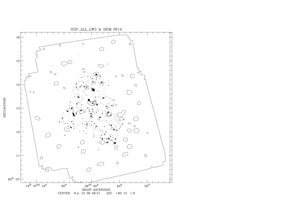
Figure 9: HDF optical f814 map (grey scale) overlaid with the LW3 contour of the 3 coadded rasters. The contour is at about the 3 $\sigma$ level. The outside contour (as defined by a minimum redundancy of 2) delimits the region where the source searching algorithm was applied.

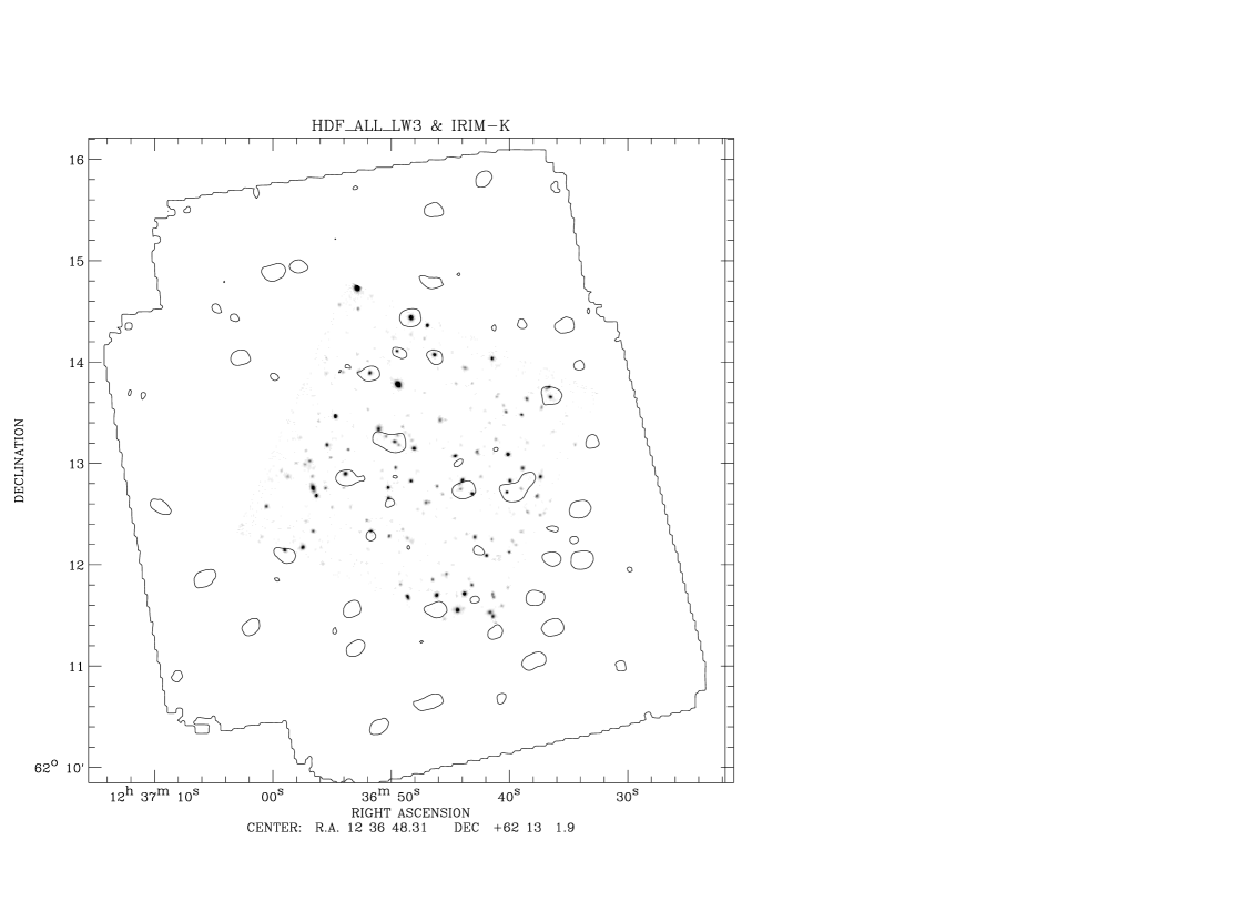
Figure 10: HDF K band near IR map (grey scale) overlaid with the LW3 contour of the same 3 coadded rasters. The contour is at about the 3 $\sigma$ level.

Essentially, the LW2 survey yields only two sources above the 4 $\sigma$ level of confidence. They both have an LW3 couterpart. We conclude that at the 60 $\,\mu{\rm Jy}\,$level, there are 2 (say at most a few) sources in the 11 arcmin² main area of the HDF, a result at odds with the numerous sources found by Goldschmidt et al. (1997). The discrepancy has been addressed by Aussel et al. (1997). We note that almost all LW2 sources have an LW3 counterpart. This small number of sources is not in disagreement with the 15 sources found in a different region but with a similar area by Taniguchi et al. (1997) at a sensitivity level twice to 3 times better than here in the same LW2 filter. The sensitivity level is here achieved with 1.7 hours of integration per sky pixel of 3 arcseconds. In the following, we concentrate on the LW3 results which, because of the larger number of sources, gives a better statistics on number counts. In the final table (6), 34 objects are above the 4 $\sigma$ limit of typically 100 to 150$\,\mu{\rm Jy}\,$in an approximate area of 25 arcmin². The best sensitivity limit quoted is obtained with an effective on-source integration time of 2.7 hours. Number counts are discussed by Aussel et al. (1998).

The overall reliability of the method can now be assessed both internally and externally:

• for the strong sources which are detected in individual rasters, the statistical significance in each of the subrasters (compare the signal-to-noise ratio S/N_1,2,3 to S/N_t in Tables 3, 4, 5) is lower than the total result but the flux estimate is in agreement with the final map flux within the error bars (the quality factors are always large)

• in the central common HDF area, the same sources are found in different completely independent rasters. Indeed by comparing Tables 3, 4, 5 and 6, one can note the overall satisfactory photometric and astrometric consistency of the sources, within the stated error bars, for example HDF-2_LW3_9, HDF-3_LW3_5 correspond to HDF_ALL_LW3_25, and HDF-2_LW3_14, HDF-3_LW3_10, HDF-4_LW3_23
  agree with HDF_ALL_LW3_33. Strictly speaking, this argument does not hold for the sources that helped in correcting the astrometry.

The complete identification, as well as the detailed comparison with the source list given by Goldschmidt et al. (1997), Rowan–Robinson et al. (1997) and Aussel et al. (1998) and by radio surveys, as well as the analysis of supplementary data taken as a repeat of LW2 observations will be dealt with in a forthcoming paper. A third external level of consistency can already be made: more than a third of the HDF LW3 sources are found in the VLA radio sample of Richards et al (1998). The analysis of Fig. 9 and Fig. 10 already reveals that, in the central HDF area, one always finds one or several bright counterparts in the optical (B magnitude less than 22). An even more clear cut case is that the sources can also be always associated with a K counterpart of relatively bright 17 to 18 magnitude, except for one source HDF_ALL_LW3_20 at the lower west border with RA=12 36 46.2 and Dec= 62 11 33.5 (confirmed in LW3 observations by the 2 rasters HDF-3_LW3 and HDF-4_LW3). This could be a good example of a galaxy very dim in the optical (29th magnitude) and near-infrared domain relative to its mid-infrared luminosity, for which no redshift can be measured except in the mid, far infrared or radio domains. Another example is HDF_ALL_LW3_24 which is associated with a radio source identified with a R_AB=23.9 elliptical galaxy by Richards et al. (1998). Table 6 gives the redshift (when available in the internet lists, Cowie et al. 1998) of the galaxy which is the brightest and nearest source (within 6 arcseconds) to a given ISOCAM source (in a simple eye-ball sense). Almost all redshifts are within the 0.5 to 1 range. We are probably seeing the PAH spectral features around $7.7\hbox{$\,\mu{\rm m}\,$}$ redshifted in the LW3 band. The fact that most of these sources are not detected in LW2 (when observed) but detected in K means that LW2 witnesses the break between stellar emission and interstellar dust emission, for the ISOCAM HDF source redshifts. Two double sources can be spotted in this table. These are HDF_ALL_LW3_13 with 15, and 27 with 29. Only one object is a star (at the border of the map) and not a galaxy: HDF_ALL_LW3_41 (see Aussel et al. 1998).

It is clear that the redundancy of the rasters plays a crucial role in assessing the reliability of sources. The reliability of our method is clearly demonstrated here on the HDF ISOCAM data, because of their large (up to 50–100) redundancy. It will be used in various other ISOCAM deep surveys, where such a redundancy cannot be afforded. It is shown here that the temporal triple beam-switch method plus a classical spatial detection on an optimally coadded map of individual measurements allow the source noise to be less than 2 parts per ten thousand of the zodiacal background (as numerically found with the present data). The method is linear and does not deal in different ways with high and low flux sources (as long as they are small compared with the zodiacal background). This is achieved with a modest-size telescope and modest-size detector array with a strong reaction to cosmic rays and with some non-linear behaviours. Finally, we note that the LW3 map is above the camera confusion limit by a factor two.