Radical Compression of
Cosmic Microwave Background Data

Abstract

Powerful constraints on theories can already be inferred from existing CMB anisotropy data. But performing an exact analysis of available data is a complicated task and may become prohibitively so for upcoming experiments with $\gtrsim 10^{4}$ pixels. We present a method for approximating the likelihood that takes power spectrum constraints, e.g., “band-powers”, as inputs. We identify a bias which results if one approximates the probability distribution of the band-power errors as Gaussian—as is the usual practice. This bias can be eliminated by using specific approximations to the non-Gaussian form for the distribution specified by three parameters (the maximum likelihood or mode, curvature or variance, and a third quantity). We advocate the calculation of this third quantity by experimenters, to be presented along with the maximum-likelihood band-power and variance. We use this non-Gaussian form to estimate the power spectrum of the CMB in eleven bands from multipole moment $\ell=2$ (the quadrupole) to $\ell=3000$ from all published band-power data. We investigate the robustness of our power spectrum estimate to changes in these approximations as well as to selective editing of the data.

1 Introduction

Measurement of the anisotropy of the Cosmic Microwave Background (CMB) is proving to be a powerful cosmological probe. Proper statistical treatment of the data—likelihood calculation—is complicated and time-consuming, and promises to become prohibitively so in the very near future. Here, we introduce approximations for this likelihood calculation which allow simple and accurate evaluation after the direct estimation of the power spectrum ($C_{\ell}$) from the data.

Although it is possible to produce constraints on cosmological parameters directly from the data, using the power spectrum as an intermediate step (e.g. Tegmark (1997)) has several advantages. The near-degeneracy of some combinations of cosmological parameters (e.g., Bond, Efstathiou & Tegmark (1997)) implies the surfaces of constant likelihood in cosmological parameter space are highly elongated, making it difficult for search algorithms to navigate (Oh, Spergel & Hinshaw, 1998). The power spectrum space is much simpler than the cosmological parameter space since each multipole moment (or band of multipole moments) is usually only weakly dependent on the others, alleviating the search difficulties. Although one still has the problem left of estimating nearly degenerate cosmological parameters from the resulting power spectrum constraints, the likelihood given the power spectrum constraints is much easier to compute than the likelihood given the map data.

Proceeding via the power spectrum also facilitates the calculation of constraints from multiple datasets. Without this intermediate step, a joint analysis may often be prohibitively complicated. Aspects particular to each experiment (e.g., offset removals, non-trivial chopping strategies) make implementation of the analysis sufficiently laborious that no one has jointly analyzed more than a handful of datasets in this manner. Reducing each dataset to a set of constraints on the power spectrum can serve as a form of data compression which simplifies further analysis. Indeed, most studies of cosmological parameter constraints from all, or nearly all, of the recent data have used, as their starting points, published power spectrum constraints, [(Lineweaver, 1997, 1998a, 1998b, 1998c; Lineweaver & Barbosa, 1998; Hancock et al., 1998); see also Tegmark (1998) and Efstathiou et al. (1998) for joint analyses with other datasets]. Since the power spectrum constraints are usually described with orders of magnitude fewer numbers than the pixelized data, we refer to this compression as “radical”.

Are there any disadvantages to proceeding via the power spectrum? To answer this question, let us consider the analysis procedure. Most analyses of CMB datasets have assumed the noise and signal to be Gaussian random variables, and to date there is no strong evidence to the contrary (although for a different view, see Ferreira, Magueijo & Gorski (1998)). The simplicity of this model of the data allows for an exact Bayesian analysis, which has been performed for almost all datasets individually. The procedure is conceptually straightforward: maximize the probability $P({\rm parameters}|{\rm data})$ over the allowed parameter space. Most often, we take the prior probability for the parameters to be constant, so this is equivalent to maximizing the likelihood, $P({\rm data}|{\rm parameters})$. Because we have assumed the noise and signal to be Gaussian, this latter is just a multivariate Gaussian in the data; the theoretical parameters enter into the covariance matrix.

Fortunately, if the theoretical signal is indeed normally distributed and in addition the signals are statistically isotropic, the power spectrum encodes all of the information about the model, and all of the constraints on the parameters of the theory can be obtained from the $C_{\ell}$ probability distribution: i.e., the likelihood as a function of some (cosmological) parameters, $a_{i}$, is just the likelihood as a function of the power spectrum determined from those parameters: $P({\rm data}|a_{i})=P({\rm data}|C_{\ell}[a_{i}])$. Thus the constraints on the power spectrum may serve as our “compressed dataset”. (If the theory is not isotropic, as may occur for nontrivial topologies (e.g., Bond, Pogosyan & Souradeep (1998)), or is non-Gaussian, then the analysis must go beyond the isotropic power spectrum.)

A problem arises though due to the fact that the uncertainties in the power spectrum determination are not Gaussian-distributed. Thus if we compress the power spectrum probability distribution to a mean (or mode—the location of the posterior maximum) and a variance, we lose the information contained in the higher order moments. One might be tempted to rely on the central limit theorem and hope that the posterior for the power spectrum is sufficiently close to a Gaussian that a simple $\chi^{2}$ procedure will suffice. This is what has been done in recent joint analyses of current CMB data (e.g., Lineweaver (1997); Lineweaver (1998a); Lineweaver (1998b); Lineweaver (1998c); Lineweaver & Barbosa (1998); Hancock et al. (1998)). and what has been advocated for the analysis of satellite data (e.g., Tegmark (1997)).

Not only is information discarded with this procedure, however—which one might think of as merely increasing the final error bars—but neglect of this effect leads to a bias (Jaffe, Knox & Bond, 1998; Bond, Jaffe & Knox, 1998; Seljak, 1997; Oh, Spergel & Hinshaw, 1998). Here we show that the information loss and its effects, such as this bias, can be greatly reduced by assuming the posterior distribution to have a specific non-Gaussian form parameterized by the likelihood maximum, the covariance matrix and a third quantity which measures the noise contribution to the uncertainty of each measured amplitude.

A relatively fast algorithm for determining the power spectrum or other parameters is the “quadratic estimator” (Tegmark, 1997; Bond, Jaffe & Knox, 1998; Oh, Spergel & Hinshaw, 1998), although it still requires $O(n^{3}_{\rm pix})$ operations, where $n_{\rm pix}$ is the number of pixels in the dataset. Our view of quadratic estimation is that, used iteratively, it is a particular method for finding the maximum of the likelihood and the parameter covariance matrix (Bond, Jaffe & Knox, 1998; Oh, Spergel & Hinshaw, 1998). We emphasize that the information loss associated with compression to a mode and covariance matrix has nothing to do with how that mode and covariance matrix are calculated. Other methods of likelihood analysis will, of course, suffer the same problems when the constraints are reduced to these two sets of quantities. In fact, the quadratic estimation algorithm has the advantage that an implementation of it as a computer code can be used (with very minor changes) to calculate the new noise contribution quantity.

In Section 2, we describe the problems generated by the non-Gaussianity of the likelihood function, and propose solutions which allow rapid and simple calculation of cosmological likelihoods for CMB data at the price of calculating only this single new parameter at each $\ell$ (or band). Bartlett et al. (1999) have used an ansatz, essentially equivalent to the equal-variance approximation of Sec. 2.2.2 to arrive at similar results.) In Section 3, we test this method via application to COBE/DMR data. In Section 4, we extend the formalism to more complicated chopping experiments and to the measurement of other amplitude parameters such as bandpowers. We apply these extensions to the Saskatoon data in Section 5, to OVRO, SP and SuZIE in Section 6, and Saskatoon combined with COBE/DMR, in Section 7.

We then apply our procedure to the more ambitious task of fitting an eleven parameter model to a compendium of all CMB results to date in Section 8. Previous explorations of parameter space have been limited to much lower dimensionality and have assumed Gaussianity (e.g., Lineweaver (1997); Lineweaver (1998a); Lineweaver (1998b); Lineweaver (1998c); Lineweaver & Barbosa (1998); Hancock et al. (1998)). The parameters are the power in eleven bins from $\ell=2$ to $\ell=3000$. We study the robustness of the resulting maximum likelihood power spectrum to assumptions about the noise contribution to the error, different binnings and selective editings of the data. The binned power spectrum, fit to the band-power data, provides an excellent tool for visualizing the combined power spectrum constraints from all the data. Such a figure should replace the usual one of all the band powers, which is much harder to interpret.

Finally, in Section 9 we discuss the results and conclude, ending with an exhortation to the community to calculate and provide the appropriate quantities for all future experiments.

Throughout, we will use $C_{\ell}$ to refer to the usual CMB power spectrum, and define

$${\cal C}_{\ell}\equiv{\ell(\ell+1)\over 2\pi}C_{\ell}.$$ (1)

2 Non-Gaussianity of the Likelihood Function

2.1 The Problem: Cosmic Bias

To illustrate the problem, consider an unrealistic “experiment” covering the whole sky with no noise. In this case, the data at pixel $p$, $\Delta_{p}$ is just the actual sky signal, $s_{p}$, and the correlation matrix, $S_{pp^{\prime}}$, is just the correlation function $c(\theta_{pp^{\prime}})$. Even in this case, the observed sky is just one realization of the underlying power spectrum. To determine these ${\cal C}_{\ell}\equiv\ell(\ell+1)C_{\ell}/(2\pi)$, we still must resort to the likelihood function. In this case,

$$-2\ln P(\Delta|{\cal C}_{\ell}) = \ln\det S({\cal C}_{\ell})+\Delta^{\dagger}S^{-1}\Delta$$ (2)

$$= \sum_{\ell}(2\ell+1)\left(\ln{\cal C}_{\ell}+{\widehat{\cal C}}_{\ell}/{\cal C}_{\ell}\right)\,,$$

up to an irrelevant additive constant. In the second line, we define the observed power spectrum of this realization as

$${\widehat{\cal C}}_{\ell}={\ell(\ell+1)\over 2\pi}\ {1\over 2\ell+1}\sum_{m}|a_{\ell m}|^{2}\,,$$ (3)

where the $a_{\ell m}$ are the spherical harmonic coefficients of the (noise-free) observed sky.

A Gaussian distribution has the following properties: it is completely specified by its mean and covariance matrix (higher moments of the distribution can be derived from these); the covariance matrix is given by the inverse of the curvature matrix (defined as ${\cal F}_{\ell\ell^{\prime}}=-{\partial^{2}\ln P(\Delta|{\cal C}_{\ell})/\partial{\cal C}_{\ell}\partial{\cal C}_{\ell^{\prime}}}$); and the curvature matrix is independent of ${\cal C}_{\ell}$. None of these properties hold for the distribution in Eq. 2, which is non-Gaussian. For a non-Gaussian distribution, it is therefore often useful to consider the ensemble average curvature, also known as the Fisher Matrix, $F\equiv\langle{\cal F}\rangle$.

What happens if, despite the non-Gaussianity of the distribution in Eq. 2, one identifies the covariance matrix with the inverse of the curvature matrix and then ignores higher order moments? The first step would be calculation of the curvature matrix:

$$-{\partial^{2}\ln P(\Delta|{\cal C}_{\ell})\over\partial{\cal C}_{\ell}\partial{\cal C}_{\ell^{\prime}}}={2\ell+1\over 2}\left(2{\widehat{\cal C}}_{\ell}/{\cal C}_{\ell}^{3}-1/{\cal C}_{\ell}^{2}\right)\delta_{\ell\ell^{\prime}}.$$ (4)

Note that, unlike for a Gaussian distribution, the curvature depends on ${\cal C}_{\ell}$. The natural remedy is to evaluate it at the peak of the likelihood, ${\widehat{\cal C}}_{\ell}$. The standard error (square root of the variance) is then given by $\delta{\cal C}_{\ell}=\sqrt{2/(2l+1)}{\cal C}_{\ell}$. Note though that, uncertainties derived in this manner are larger if ${\widehat{\cal C}}_{\ell}$ has fluctuated upward from the underlying “real” value and smaller for a downward fluctuation. If, in addition, we ignore higher order moments of the distribution, then upward fluctuations are given less weight than downward fluctuations, resulting in a downward bias for the overall power spectrum amplitude. It is generally the lowest multipole moments constrained by an observation that have the most non-Gaussian distributions. As has been seen (Bunn & White, 1997; Bond, Jaffe & Knox, 1998) and will be seen again below, this may contribute to some of the confusion in the community regarding the so-called anomalous value of the COBE quadrupole.

In the presence of noisy data over partial areas of the sky, the likelihood is no longer so simple, and must be laboriously calculated (e.g., Bond (1994);Bunn & White (1997);Bond & Jaffe (1998a);Bond & Jaffe (1998b)). In Fig. 1 we show the actual likelihood for the COBE quadrupole and other multipoles, along with the Gaussian that would be assumed given the curvature matrix calculated from the data. The figures show another way of understanding the bias introduced by assuming Gaussianity: upward deviations from the mean (which is not actually the mean of the non-Gaussian distribution, but the mode) are overly disfavored by the Gaussian distributions while downward ones are overly probable. For example, the standard-CDM value of ${{\cal C}}_{2}=770\mu{\rm K}^{2}$ is only 0.2 times less likely than the most likely value of $150\mu{\rm K}^{2}$ but it seems like a 5-sigma excursion ($4\times 10^{-6}$ times less likely) based on the curvature alone.

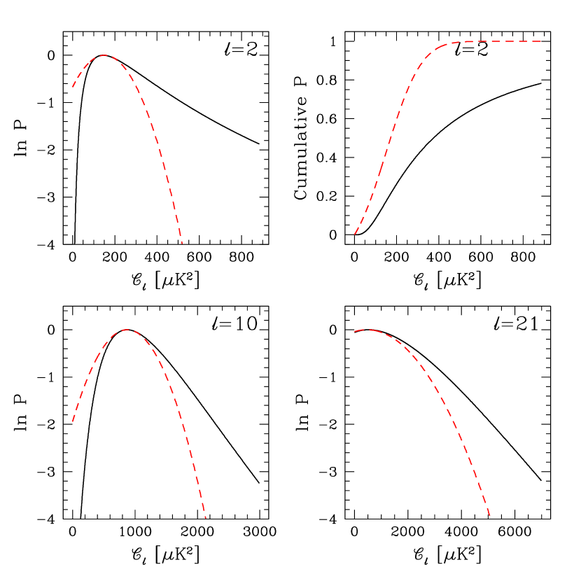
Figure 1: DMR Likelihoods $P(\Delta|{\cal C}_{\ell}$) for various values of $\ell$, as marked. The horizontal axis is ${\cal C}_{\ell}=\ell(\ell+1)C_{\ell}/(2\pi)$. The upper right panel gives the cumulative probability. The solid (black) line is the full likelihood calculated exactly. The dashed (red) line is the Gaussian approximation about the peak.

Although it is extremely pronounced in the case of the quadrupole this is a problem that plagues all CMB data: the actual distribution is skewed to allow larger positive excursions than negative. The full likelihood “knows” about this and in fact takes it into account; however, if we compress the data to observed ${\cal C}_{\ell}\pm\sigma_{\ell}$ (or even observed ${\cal C}_{\ell}$ and a correlation matrix $M_{\ell\ell^{\prime}}$) we lose this information about the shape of the likelihood function. Because of its relation to the well-known phenomenon of cosmic variance, we choose to call this problem one of cosmic bias.

We emphasize that cosmic bias can be important even in high-S/N experiments with many pixels. We might expect the central limit theorem to hold in this case and the distributions to become Gaussian. Indeed they do, at least near the peak. However, the central limit theorem does not guarantee that the tails of the distribution will approach those of a Gaussian as rapidly as does the region near the peak and there is the danger that a few seemingly discrepant points are given considerably more weight than they deserve. Cosmic bias has also been noted in previous work (Bond, Jaffe & Knox, 1998; Seljak, 1997; Oh, Spergel & Hinshaw, 1998).

Putting the problem a bit more formally, we see that even in the limit of infinite signal-to-noise we cannot use a simple $\chi^{2}$ test on ${\cal C}_{\ell}$ estimates; such a test implicitly assumes a Gaussian likelihood. Unlike the distribution discussed here, a Gaussian would have constant curvature ($\delta{\cal C}_{\ell}={\rm constant}$), rather than $\delta{\cal C}_{\ell}\propto{\cal C}_{\ell}$ as illustrated here.

We emphasize that the problem as outlined here is easily solved in principle: just calculate using the full likelihood function. Unfortunately, this is more easily said than done—direct calculation of the likelihood function takes $O(n_{p}^{3})$ operations per parameter-space point. For the $n_{p}\gtrsim 10^{5}$ datasets already coming, this is prohibitively expensive. Indeed, it is not even clear how to perform the operations necessary even to find the likelihood peak and variance in a reasonable time (Bond, Jaffe & Knox, 1998; Oh, Spergel & Hinshaw, 1998). It is likely that other forms of data compression and/or new algorithms will be necessary even at this stage of the analysis. Signal-to-noise Eigenmodes, discussed in Appendix A, have been suggested as a useful compression tool (Tegmark, Taylor & Heavens, 1997; Jaffe, Knox & Bond, 1998) and used in some analyses (Bond & Jaffe, 1998a, b; Bunn & Sugiyama, 1995; Bunn & White, 1997).

Instead, we must find efficient ways to approximate the likelihood function based on minimal information. In the rest of this paper, we discuss two approximations, each motivated by different aspects of our knowledge of the likelihood function. Each requires only knowledge of the likelihood peak and curvature (or variance) as well as a third quantity related to the noise properties of the experiment. Alternately, for already-calculated likelihood functions, each approximation gives a functional form for fitting with a small number of parameters.

2.2 The solution: approximating the likelihood

2.2.1 Offset lognormal distribution

We already know enough about the likelihood to see a solution to this problem. For a given multipole $\ell$, there are two distinct regimes of likelihood. Add uniform pixel noise and a finite beam to the simple all-sky “experiment” considered above. Now, the likelihood has contributions from the signal, $a_{\ell m}$, and the noise, $n_{\ell m}$ (after transforming again to spherical harmonics).

$$-2\ln P(\Delta|{\cal C}_{\ell})=$$

$$\sum_{\ell}(2\ell+1)\left[\ln\left({\cal C}_{\ell}B_{\ell}^{2}+{\cal N}_{\ell}\right)+{{\widehat{\cal D}}_{\ell}\over{\cal C}_{\ell}B_{\ell}^{2}+{\cal N}_{\ell}}\right]$$ (5)

(as usual up to an irrelevant additive constant), with ${\cal N}_{\ell}=\ell(\ell+1)N_{\ell}/(2\pi)$, where $N_{\ell}=\langle|n_{\ell m}|^{2}\rangle$ is the noise power spectrum in spherical harmonics, and ${\widehat{\cal D}}_{\ell}\equiv[\ell(\ell+1)/(2\pi)]\ \sum_{m}|a_{\ell m}|^{2}/(2\ell+1)$ is the power spectrum of the full data (noise plus beam-smoothed signal); we have written it as a different symbol from above to emphasize the inclusion of noise and again use script lettering to refer to quantities multiplied by $\ell(\ell+1)/(2\pi)$.

Now, the likelihood is maximized at ${\cal C}_{\ell}=({\widehat{\cal D}}_{\ell}-{\cal N}_{\ell})/B_{\ell}^{2}$ and the curvature about this maximum is given by

$${\cal F}^{({\cal C})}_{\ell\ell^{\prime}}=-{\partial^{2}\ln P(\Delta|{\cal C}_{\ell})\over\partial{\cal C}_{\ell}\partial{\cal C}_{\ell^{\prime}}}={2\ell+1\over 2}\left({\cal C}_{\ell}+{\cal N}_{\ell}/B_{\ell}^{2}\right)^{-2}\delta_{\ell\ell^{\prime}}$$ (6)

so the error (defined by the variance) on a ${\cal C}_{\ell}$ is

$$\delta{\cal C}_{\ell}=\left({\cal C}_{\ell}+{\cal N}_{\ell}/B_{\ell}^{2}\right)/\sqrt{\ell+1/2}.$$ (7)

Note that in this expression there is once again indication of a bias if we assume Gaussianity: upward fluctuations have larger uncertainty than downward fluctuations. But this is not true for $Z_{\ell}$ where $Z_{\ell}$ is defined so that $\delta Z_{\ell}\propto\delta{\cal C}_{\ell}/({\cal C}_{\ell}+{\cal N}_{\ell}/B_{\ell}^{2})$. More precisely, $Z_{\ell}\equiv\ln({\cal C}_{\ell}+{\cal N}_{\ell}/B_{\ell}^{2})$. Since $\delta Z_{\ell}$ is proportional to a constant, our approximation to the likelihood is to take $Z_{\ell}$ as normally distributed. That is, we approximate

$$-2\ln P(\Delta|{\cal C}_{\ell})=\sum_{\ell\ell^{\prime}}Z_{\ell}M^{(Z)}_{\ell\ell^{\prime}}Z_{\ell^{\prime}}$$ (8)

(up to a constant) where $M^{(Z)}_{\ell\ell^{\prime}}=({\cal C}_{\ell}+x_{\ell})M^{({\cal C})}_{\ell\ell^{\prime}}({\cal C}_{\ell^{\prime}}+x_{\ell^{\prime}})$ where $M^{({\cal C})}$ is the weight matrix (covariance matrix inverse) of the ${\cal C}_{\ell}$, usually taken to be the curvature matrix. We refer to Eq. 8 as the offset lognormal distribution of ${\cal C}_{\ell}$. Somewhat more generally we write

$$Z_{\ell}=\ln({\cal C}_{\ell}+x_{\ell})$$ (9)

for some constant $x_{\ell}$, which for the case at hand is $x_{\ell}={\cal N}_{\ell}/B_{\ell}^{2}$.

It is illustrative to derive the quantity $Z_{\ell}$ in a somewhat more abstract fashion. We wish to find a change of variables from ${\cal C}_{\ell}$ to $Z_{\ell}$ such that the curvature matrix is a constant:

$${\partial{\cal F}^{(Z)}_{\ell\ell^{\prime}}\over\partial Z_{\ell}}=0.$$ (10)

That is, we want to find a change of variables such that

$$\left({\cal F}^{(Z)}\right)^{-1}_{LL^{\prime}}=\sum_{\ell\ell^{\prime}}{\partial Z_{L}\over\partial{\cal C}_{\ell}}\left({\cal F}^{({\cal C})}\right)^{-1}_{\ell\ell^{\prime}}{\partial Z_{L^{\prime}}\over\partial{\cal C}_{\ell^{\prime}}}$$ (11)

is not a function of $Z$. We immediately know of one such transformation which would seem to do the trick:

$${\partial Z_{L}\over\partial{\cal C}_{\ell}}={\cal F}_{L\ell}^{1/2}$$ (12)

where the ${1/2}$ indicates a Cholesky decomposition or Hermitian square root. In general, this will be a horrendously overdetermined set of equations, $N^{2}$ equations in $N$ unknowns. However, we can solve this equation in general if we take the curvature matrix to be given everywhere by the diagonal form for the simplified experiment we have been discussing (Eq. 6). In this case, the equations decouple and lose their dependence on the data, becoming (up to a constant factor)

$${dZ_{\ell}\over d{\cal C}_{\ell}}=\left({\cal C}_{\ell}+{\cal N}_{\ell}/B_{\ell}^{2}\right)^{-1}.$$ (13)

The solution to this differential equation is just what we expected,

$$Z_{\ell}=\ln({\cal C}_{\ell}+{\cal N}_{\ell}/B_{\ell}^{2})$$ (14)

with correlation matrix

$$\left({\cal F}^{(Z)}\right)^{-1}_{\ell\ell^{\prime}}={\left({\cal F}^{({\cal C})}\right)^{-1}_{LL^{\prime}}\over\left({\cal C}_{L}+{\cal N}_{L}/B_{L}^{2}\right)\left({\cal C}_{L^{\prime}}+{\cal N}_{L^{\prime}}/B_{L^{\prime}}^{2}\right)}$$ (15)

where $\ell=L$ and $\ell^{\prime}=L^{\prime}$. Please note that we are calculating a constant correlation matrix; the ${\cal C}_{\ell}$ in the denominator of this expression should be taken at the peak of the likelihood (i.e., the estimated quantities).

We emphasize that, even for an all-sky continuously and uniformly sampled experiment (for which Eq. 6 is exact), this Gaussian form, Eq. 8, is only an approximation, since the curvature matrix is given by Eq. 6 only at the peak. Nonetheless we expect it to be a better approximation than a naive Gaussian in ${\cal C}_{\ell}$ (which we note is the limit $x_{\ell}\to\infty$ of the offset lognormal).

We also note that there is another approximation involved in this expression: by choosing just a single independent change of variable for each $\ell$ we assume that the correlation structure is unchanged as you move away from the likelihood peak.

Often a very good approximation to the curvature matrix is its ensemble average, the Fisher matrix, $F\equiv\langle{\cal F}\rangle$. Below, unless mentioned otherwise, we use the Fisher matrix in place of the curvature matrix. However, we will see that in our application to the Saskatoon data, the differences between the curvature matrix and Fisher matrix can be significant.

2.2.2 The Equal Variance Approximation

In this subsection we consider an alternate form for the likelihood function ${\cal L}\propto P(\Delta|{\cal C}_{\ell})$ that is sometimes a better approximation than the offset-lognormal form. The approximation is exact in the limit that the observations can be decomposed into modes that are independent, with equal variances. For example, for a switching experiment in which the temperature of $G$ pixels are measured, with the same noise $\sigma_{N}$ at each point, and such that each pixel is far enough from the others that there is no correlation between the points, the likelihood can be written as

$$\ln{\cal L}=-G/2\left[\ln\left(\sigma_{T}^{2}+\sigma_{N}^{2}\right)+{\sum_{i}d_{i}^{2}/G\over\sigma_{T}^{2}+\sigma_{N}^{2}}\right]$$ (16)

where $\sigma_{T}^{2}$ is such that $C_{T,ij}=\sigma_{T}^{2}\delta_{ij}$ and $d_{i}$ are the pixel temperatures. The independent pixel idealization was very close to the case for the OVRO experiment, and, as we show in Section 6, the calculated likelihood is well approximated by this equation. The maximum likelihood occurs at a signal amplitude ${\widehat{\sigma}}_{\rm T}$ which is related to the data by ${\widehat{\sigma}}_{\rm T}^{2}=\sum d_{i}^{2}/G-\sigma_{N}^{2}$.

If we define $Z=\ln\left(\sigma_{T}^{2}+x\right)$, $\widehat{Z}=\ln\left(\widehat{\sigma}_{T}^{2}+x\right)$, and $x=\sigma_{N}^{2}$ then we can rewrite Eq. 16 in a form that will be useful for relating it to the previous offset- lognormal form:

$$\ln{\cal L}/{\widehat{\cal L}} = -{G\over 2}\left[e^{-(Z-{\widehat{Z}})}-\left(1-(Z-{\widehat{Z}})\right)\right].$$ (17)

Note that if we consider only a single $\ell$ then the above form applies to Eq. 2.2.1 as well, with $G=2\ell+1$ and $Z=\ln\left({\cal C}_{\ell}+x_{\ell}\right)$. We know this should be the case since the likelihood of Eq. 2.2.1 (for a single $\ell$) is also one for independent modes ($a_{lm}$) with equal variances (${\cal C}_{\ell}+x_{\ell}$). If we fix $G$ and $x$ for each mode (e.g., band of $\ell$), we refer to this as the “equal variance approximation.” Also note that the first term in the expansion of Eq. 17 in $Z-\widehat{Z}$ is $-G/2\left(Z-\widehat{Z}\right)^{2}$, which with the identification, $G=2{\cal F}^{(Z)}$, is the offset-lognormal form. Thus when the modes have equal variance and are independent, then the offset lognormal form is simply the first term in a Taylor expansion of the equal-variance form. An advantage of the full form is that the asymptotic form $-(G/2)(Z-{\widehat{Z}})$ linear in $Z$ for large signal amplitudes holds (and thus gives a power law rather than exponential decay in ${\cal L}$), whereas the offset lognormal is dominated by the $Z^{2}$. An advantage of the offset-lognormal form is that it does not require the existence of equal and independent modes. Figure 2 shows that for the range of relevance for the likelihoods for DMR, the offset lognormal and the equal/independent variance likelihood approximations are quite close over the dominant 2-sigma falloff from maximum. We have found this to generally be true.

For either form, three quantities need to be specified, the noise-related offset $x$, ${\widehat{Z}}$ and $G$. Given $x$, ${\widehat{Z}}$ is determined from the maximum likelihood and $G$ can be determined from the curvature of the likelihood. One could also specify the amplitudes ${\cal C}$ at three points, e.g., at the maximum and the places where ${\cal L}/{\widehat{\cal L}}$ falls by $e^{-1/2}$, the upper and lower one-sigma errors if the distribution were fit on either side by a Gaussian. Forcing the approximation to pass through these points enforces values of $x$, ${\widehat{Z}}$ and $G$.

In Section 8, we apply these approximations to power spectrum estimation from current data for which the practice has been to quote a signal amplitude with upper and lower one-sigma errors, say ${\widehat{\cal C}}$, ${\cal C}_{u}$ and ${\cal C}_{d}$. Often these are Bayesian estimates, determined by choosing a prior probability for ${\cal C}$ and integrating the likelihood. Sometimes the $e^{-1/2}$ points are given, which are slightly easier to implement in fitting for $x$ and $G$. Since the tail of Eq. 17 is quite pronounced, resulting in a dramatic asymmetry in ${\cal L}$ between the up and down sides of the maximum even in the $Z$ variable, we have found that just using the second derivative of the likelihood or the Fisher matrix approximation to it to fix $G$ is not as good as assuming the offset lognormal and requiring that the functional forms match at the upper $e^{-1/2}$ point. Thus, if the error $\sigma_{\cal C}=1/\sqrt{{\cal F}^{({\cal C})}}$ is from the curvature or Fisher matrix, then we prefer the choice

$$G=\left[e^{-\sigma_{Z}}-(1-\sigma_{Z})\right]^{-1}\,,\ \sigma_{Z}={\sigma_{\cal C}\over{\widehat{\cal C}}+x}={1\over\sqrt{{\cal F}^{(Z)}}}$$ (18)

rather than the curvature form $G=2/\sigma_{Z}^{2}$, or the $[{\rm cosh}(\sigma_{Z})-1]^{-1}$ average of the $\pm 1/2$ widths. This is what was done in Fig. 2, and in all subsequent figures.

Fig. 2 shows that a linear $-GZ/2$ asymptote in the log-likelihood is not always correct and sometimes the lognormal does better. That the tail often declines faster can be understood in terms of an effective number of modes $G({\cal C}^{-1})$ which increases as ${\cal C}$ increases. To demonstrate this, it is useful to consider the likelihood behavior for “signal-to-noise” eigenmodes, which are linear combinations of the pixelized data which make them statistically independent for Gaussian signals and noise. The data is then characterized by observed amplitudes $d_{k}$, with a noise contribution transformed to give unity variance, and a signal contribution with amplitude ${\cal C}\lambda_{k}$, in terms of a “signal-to-noise” eigenvalue $\lambda_{k}$ and an overall amplitude ${\cal C}$. Such transformations have been much discussed in the literature (e.g., Bond (1994);Bunn & Sugiyama (1995);Bunn & White (1997);Bond, Jaffe & Knox (1998)), and we will not go into the details here; for more details on using this formalism to examine the overall form of the likelihood function, see Appendix A.

The cases in which we expect Eq. 17 to be a good approximation are those in which the eigenmodes have a broad region over which $\lambda$ varies slowly and a very rapid falloff towards zero beyond. This is exact for the independent pixel points described above, with $\lambda=\sigma_{T}^{2}/\sigma_{N}^{2}$ the same for all $G$ modes. If there were a number of frequency channels as well as pixels, only the linear combinations which are flat in thermodynamic temperature have this $\lambda$, and the rest are zero. For cases where the equal variance approximation is not exact, the signal-to-noise modes will have different eigenvalues $\lambda$. One might then take an effective $G$ to be the number of modes with $\lambda>1$ or some other cutoff (since these are the ones that have greater signal than noise). However, then $G$ grows as ${\cal C}_{\ell}$ increases, altering the power-law tail.

Thus, the very general approach of “signal-to-noise” eigenmodes has allowed us to understand that the simple law with an effective $G$ will usually overshoot the high ${\cal C}$ tail somewhat, even though it fits very well to 1-sigma, and usually beyond. The offset lognormal form, motivated by it, could err on either side, since it would presuppose a specific sort of increase in the number of eigenmodes contributing. Fortunately either approximation seems to work well enough to allow accurate parameter estimation from a very small set of numbers.

3 Application to COBE/DMR

We first apply these methods to the anisotropy measurements of the DMR instrument on the COBE satellite (Bennett et al., 1996). The DMR instrument actually measured a complicated set of temperature differences $60^{\circ}$ apart on the sky, but the data were reported in the much simpler form of a temperature map, along with appropriate errors (which we have expanded to take into account correlations generated by the differencing strategy, as treated in Bond (1994), following Lineweaver & Smoot (1993). The calculation of the theoretical correlation matrix includes the effects of the beam, digitization of the time stream, and an isotropized treatment of pixelization, using the table given by Kneissel & Smoot (1993), modified for resolution 5. We use a weighted combination of the 31, 53 and 90 GHz maps. Because most of the information in the data is at large angular scales, we use the maps degraded to “resolution 5” which has 1536 pixels. Further, we cannot of course observe the entire CMB sky; we use the most recent galactic cut suggested by the COBE/DMR team (Bennett et al., 1996), leaving us with 999 pixels to analyze. We use the galactic, as opposed to ecliptic, pixelization.

Before we can apply our procedure to COBE/DMR, we must discuss how to deal with the partial sky coverage of any real CMB experiment. To a good approximation, the COBE/DMR Fisher matrix can be written as (e.g., Knox (1995);Jungman et al. (1996);Bond, Jaffe & Knox (1998);Hobson & Magueijo (1996))

$$F^{({\cal C})}_{\ell\ell^{\prime}}=f_{\rm sky}{2\ell+1\over 2}\left[{\cal C}_{\ell}+{\ell(\ell+1)\over 2\pi wB_{\ell}^{2}}\right]^{-2}\delta_{\ell\ell^{\prime}}.$$ (19)

In the language of our new procedure, this means that we still expect to be able to approximate the likelihood as a Gaussian in the same $Z_{\ell}=\ln({\cal C}_{\ell}+x_{\ell})$, but now we can only approximate the term $x_{l}\simeq\ell(\ell+1)/[2\pi wB^{2}(\ell)]$, where $w$ is the weight per solid angle of the experiment. In terms of the total weight, $W$, of the experiment, $w=W/(4\pi f_{\rm sky})$. A more detailed approximation for a particular experiment might be possible, but as we will see below, this expression does extremely well in reproducing the full non-Gaussian likelihood.

We have calculated the maximum-likelihood power spectrum and its error (Fisher) matrix using the quadratic estimator procedure of (Bond, Jaffe & Knox, 1998). With knowledge of the COBE/DMR beam (Bennett et al., 1996) along with the noise properties of the experiment, we can calculate the necessary quantity $x_{\ell}$. For COBE/DMR, we have an average inverse weight per solid angle of $w^{-1}=9.5\times 10^{-13}$ (equivalent to an RMS noise of $22\;\mu{\rm K}$ on $7^{\circ}\times 7^{\circ}$ pixels).

With these numbers, we show the full likelihood in comparison to the “naive Gaussian” approximation, as well as our offset lognormal ansatz. While the naive Gaussian approximation consistently overestimates the likelihood below the peak and underestimates it above the peak, the lognormal form reproduces the full expression extremely well in both regimes.

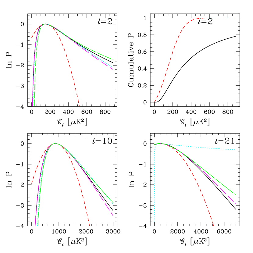
Figure 2: Full and approximate COBE/DMR likelihoods $P(\Delta|{\cal C}_{\ell})$ for various values of $\ell$, as marked. The horizontal axis is ${\cal C}_{\ell}=\ell(\ell+1)C_{\ell}/(2\pi)$. The upper right panel gives the cumulative probability. The solid (black) line is the full likelihood calculated exactly. The short-dashed (red) line is the Gaussian approximation about the peak. The dotted (cyan) line is a Gaussian in $\ln{{\cal C}_{\ell}}$; the dashed (magenta) line is a Gaussian in $\ln{({\cal C}_{\ell}+x_{\ell})}$, as discussed in the text. The dot-dashed (green) line is the equal-variance approximation.

The Gaussian form of the offset lognormal form makes using the power spectrum estimates for parameter estimation very simple: we evaluate a $\chi^{2}$ in the quantity $Z_{\ell}$ rather than ${\cal C}_{\ell}$ (although the model is now nonlinear in the spectral parameters).

Figure 3: Exact and approximate likelihood contours for COBE/DMR, for the cosmological parameters $n_{s}$ and $\sigma_{8}$ (with otherwise standard CDM values). Contours are for ratios of the likelihood to its maximum equal to $\exp{-\nu^{2}/2}$ with $\nu=1,2,3$. Upper panel is for the full likelihood (dashed) and its offset lognormal approximation as a Gaussian in $\ln{({\cal C}_{\ell}+x_{\ell})}$ (solid; see text); lower panel shows the full likelihood and its approximation as a Gaussian in ${\cal C}_{\ell}$.

Again, we see how well our offset lognormal ansatz performs; it reproduces the peak and errors on the parameters. In particular, it eliminates the “cosmic bias” discussed above, finding essentially the correct amplitude, $\sigma_{8}$ for each shape probed, unlike the naive Gaussian in ${\cal C}_{\ell}$, which consistently underestimates the amplitude. Of course, far from the likelihood peak, even the offset lognormal form misrepresents the detailed likelihood structure since no Gaussian correctly represents the softer tails of the real distribution, which goes asymptotically as the power law ${\cal C}_{\ell}^{-1/2}$; the offset lognormal approximation is asymptotically lognormal with a much steeper descent; the equal-variance form can in principle reproduce the asymptotic form better. This behavior can be important for the case of upper limits, i.e., when the likelihood peak is at ${\cal C}_{\ell}=0$. We discuss this special case in Section 6.

4 General Treatment

4.1 Chopping Experiments

We wish to generalize this procedure to the case of experiments that are not capable of estimating individual multipole moments and/or chopping experiments. By chopping experiments, which have been the norm until very recently, we mean those that rather than report the temperature at various positions on the sky, report more complicated linear combinations, with a sky signal given by

$$s_{i}=\int d^{2}{\hat{x}}\;H_{i}({\hat{x}}){\Delta T\over T}({\hat{x}})=\sum_{\ell m}H_{i,\ell m}a_{\ell m}$$ (20)

for some beam and switching function $H({\hat{x}})$; $H_{i,\ell m}$ and $a_{\ell m}$ are the spherical-harmonic transforms of $H$ and the temperature, respectively. This induces a signal correlation matrix given by

$$C_{Tii^{\prime}}=\langle s_{i}s_{i^{\prime}}\rangle=\sum_{\ell}{\ell+1/2\over\ell(\ell+1)}W_{ii^{\prime}}(\ell){\cal C}_{\ell}.$$ (21)

Here, the window function matrix, $W_{ii^{\prime}}(\ell)$, generalizes the beam $B_{\ell}^{2}$ of a mapping experiment and is given by

$$W_{ii^{\prime}}(\ell)={4\pi\over 2\ell+1}\sum_{m}H_{i,\ell m}H^{*}_{i^{\prime},\ell m}$$ (22)

(this should not be confused with the “window function,” given by ${\bar{W}}_{\ell}=\sum_{i}W_{ii}(\ell)/N_{\rm pix}$.) Moreover, for many experiments, the noise structure can be considerably more complicated, and may not be reducible to a simple noise correlation function or power spectrum (that is, correlations in the noise may not just be functions of the distance between points); instead, we may have to specify a general noise matrix

$$C_{Nii^{\prime}}=\langle n_{i}n_{i^{\prime}}\rangle$$ (23)

How can we generalize our previous procedure to account for this more complicated correlation structure? We will take the general offset lognormal form of the likelihood, a Gaussian in $Z_{\ell}=\ln({\cal C}_{\ell}+x_{\ell})$, as our guide. We have already noted that in the case of incomplete sky coverage, or inhomogeneous noise, Eq. 12 has no solution. Thus we are only searching for a reasonable ansatz to try for $x_{\ell}$.

We begin by noting that $x_{\ell}$ represents the noise contribution to the error. For the full-sky case the ratio ${\cal C}_{\ell}/x_{\ell}$ is the ratio of the signal contribution to the error to the noise contribution to the error:

$${\cal C}_{\ell}/x_{\ell}={(F^{-1/2}_{ll})_{\rm signal}\over(F^{-1/2}_{ll})_{\rm noise}}$$ (24)

since $(F^{-1/2}_{ll})_{\rm signal}=\sqrt{2/(2\ell+1)}{\cal C}_{\ell}$ and $(F^{-1/2}_{ll})_{\rm noise}=\sqrt{2/(2\ell+1)}{\cal N}_{\ell}/B_{\ell}^{2}=\sqrt{2/(2\ell+1)}x_{\ell}$. Writing ${\cal C}_{\ell}/x_{\ell}$ in Eq. 24 in terms of Fisher matrices allows us to generalize to arbitrary experiments.

Before writing down the general procedure, we must introduce a little more notation. Instead of estimating every ${\cal C}_{\ell}$, we estimate the binned power spectrum ${\cal C}_{B}\equiv\sum_{\ell\in B}{\cal C}_{\ell}/\sum_{\ell\in B}1$, in bins labeled by $B$. Let $C_{T,B}$ be the contribution to the signal covariance matrix from bin $B$, i.e., $C_{T,Bij}=\sum_{\ell\in B}{\cal C}_{B}W_{ij}(\ell)/\ell$. The Fisher matrix for ${\cal C}_{B}$ (whose inverse gives the covariance matrix for the uncertainty in ${\cal C}_{B}$) is given by

$$F^{({\cal C})}_{BB^{\prime}}={\rm Tr}\left(C^{-1}C_{T,B}C^{-1}C_{T,B^{\prime}}\right)/({\cal C}_{B}{\cal C}_{B^{\prime}})$$ (25)

where $C$ is the total covariance matrix, $C=C_{T}+C_{N}$. Of course, in the limit of no noise, $C=C_{T}$ and in the limit of no signal, $C=C_{N}$. Thus Eq. 24 generalizes to

$${\cal C}_{B}/x_{B}=\sqrt{{\rm Tr}\left(C_{N}^{-1}C_{T,B}C_{N}^{-1}C_{T,B}\right)\over{\rm Tr}\left(C_{T}^{-1}C_{T,B}C_{T}^{-1}C_{T,B}\right)}.$$ (26)

Evaluation of the denominator of Eq. 26 is sometimes difficult, as practical shortcuts in the calculation of the window function matrix may make it singular or give it negative eigenvalues. To avoid this calculation, we sometimes generalize the expression for $x_{\ell}$ by noting that for a homogeneously sampled, full-sky map:

$$(F_{\ell\ell}^{-1/2})_{\rm signal}=F_{\ell\ell}^{-1/2}-(F_{\ell\ell}^{-1/2})_{\rm noise}$$ (27)

and therefore replace Eq. 26 with

$${\cal C}_{B}/x_{B}=\sqrt{{\rm Tr}\left(C_{N}^{-1}C_{T,B}C_{N}^{-1}C_{T,B}\right)\over{\rm Tr}\left(C^{-1}C_{T,B}C^{-1}C_{T,B}\right)}-1.$$ (28)

(For the all-sky, uniform noise case, $x_{B}$ thus defined will be independent of ${\cal C}_{B}$; in a realistic experiment this will no longer hold. In practice, we expect that the correlation matrix at the likelihood peak would give the best value for $x_{B}$.)

Alternatively, we sometimes use Eq. 26 but make use of the approximation

$${\rm Tr}\left(C_{T}^{-1}C_{T,B}C_{T}^{-1}C_{T,B}\right)=\sum_{\ell\in B}(2\ell+1)f_{\rm sky}$$ (29)

which is exact for maps in the limit $f_{\rm sky}\rightarrow 1$.

To summarize, our offset lognormal ansatz is to take $Z_{B}=\ln({\cal C}_{B}+x_{B})$ as Gaussian distributed, with $x_{B}$ calculated from Eq. 28 and covariance matrix given by the inverse of

$$F^{(Z)}_{BB^{\prime}}=Z_{B}Z_{B^{\prime}}F^{({\cal C})}_{BB^{\prime}}\ \ {\rm no}\ {\rm sum}.$$ (30)

Alternately, we can use these same quantities in the equal-variance form of Eqs. 16–18.

4.2 Bandpowers

Most observational power spectrum constraints to date are reported as “band-powers” rather than as estimates of the power in a power-spectrum bin, as we have been assuming above. These band-powers are the result of assuming a given shape for the power spectrum and then using one particular modulation of the data to determine the amplitude. With ${\cal C}_{\ell}$ thus fixed, the band-power, ${\cal C}_{BP}$, is given by

$${\cal C}_{BP}={\sum_{\ell}{\ell+1/2\over\ell(\ell+1)}{\bar{W}}_{\ell}{\cal C}_{\ell}\over\sum_{\ell}{\ell+1/2\over\ell(\ell+1)}{\bar{W}}_{\ell}}\simeq{\sum_{\ell}{\bar{W}}_{\ell}{\cal C}_{\ell}/\ell\over\sum_{\ell}{\bar{W}}_{\ell}/\ell}\,,$$ (31)

with ${\bar{W}}_{\ell}$ given by the trace of the window function matrix. To find $x_{BP}$, replace $C_{T,B}$ with $C_{T}$ in Eq. 28.

Note that in order to compare this observationally-determined number, ${\cal C}_{\rm BP}$, with other theories, specified by different ${\cal C}_{l}$s with different shapes and amplitudes, we need a means for calculating the expected value of ${\cal C}_{\rm BP}$, $\langle{\cal C}_{\rm BP}\rangle$, given an arbiratry ${\cal C}_{l}$. It has been often assumed that $\langle{\cal C}_{\rm BP}\rangle$ for arbitrary ${\cal C}_{l}$ is also given by the right-hand side of Eq. 31. However, this is only strictly true in the case of a diagonal signal covariance matrix. The generalization to the case of non-diagonal signal matrices is discussed in Bond, Jaffe & Knox (1998) and Knox (1999).

4.3 Linear Combinations

Nothing we have derived so far restricts us to the likelihood as a function of ${\cal C}_{\ell}$ per se; any other measure of amplitude will also have a likelihood in this form. That is, we write a general amplitude as

$$\sigma_{i}^{2}=\sum_{\ell}f_{i}(\ell){\cal C}_{\ell}$$ (32)

for some arbitrary filter or filters, $f_{i}(\ell)$, and ${\cal C}_{\ell}=\ell(\ell+1)C_{\ell}/(2\pi)$ as usual. This filter could be, for example, one designed to make the uncertainties in the $\sigma_{i}^{2}$ uncorrelated, as in the following section.

What is the likelihood for this amplitude, rather than ${\cal C}_{\ell}$ at a single $\ell$? We first change variables from ${\cal C}_{\ell}$ to $\sigma_{i}$ as in Eq. 11. If we choose window functions that do not overlap in $\ell$, the inverse Fisher matrix then becomes

$$F^{-1}_{ii^{\prime}}=\sum_{\ell\ell^{\prime}}f_{i}(\ell)F^{-1}_{\ell\ell^{\prime}}f_{i^{\prime}}(\ell^{\prime}).$$ (33)

If the original (${\cal C}_{\ell}$) Fisher matrix has the simple form of Eq. 6, then we see that we can just filter the individual terms in any of the ensuing equations with the same $f_{i}$ and our ansatz will still hold. Explicitly, we would expect the variable

$$Z_{i}=\ln\left[\sigma^{2}_{i}+\sum_{\ell}f_{i}(\ell)x_{\ell}\right]$$ (34)

to be distributed as a Gaussian for the offset lognormal form; for the equal-variance form the generalization is clear.

4.4 Orthogonal Bandpowers

We can apply this to a particularly useful set of linear combinations, the so-called orthogonal bandpowers (Bond, Jaffe & Knox, 1998; Tegmark, 1997; Hamilton, 1997a, b; Tegmark & Hamilton, 1998). If we have a set of spectral measurements ${\cal C}_{B}$ in bands $B$ with a weight matrix $M_{BB^{\prime}}=F_{BB^{\prime}}=\langle\delta{\cal C}_{B}\delta{\cal C}_{B^{\prime}}\rangle$, we can form a new set of measurements which have a diagonal error matrix by applying a transformation like $D_{B}=M^{1/2}_{BB^{\prime}}{\cal C}_{B^{\prime}}=F^{1/2}_{BB^{\prime}}{\cal C}_{B^{\prime}}$. The $1/2$ power represents any matrix such as the Cholesky decomposition or Hermitian square root which satisfies $A^{1/2}(A^{1/2})^{T}=A$. These linear combinations will have the property that $\langle\delta{D}_{B}\delta{D}_{B^{\prime}}\rangle=\delta_{BB^{\prime}}$ (note the similarity to the calculations of Section 2.2). For calculating the “naive” quantity,

$$\chi^{2} = \sum_{BB^{\prime}}({\cal C}_{B}-{\widehat{\cal C}}_{B})M_{BB^{\prime}}({\cal C}_{B^{\prime}}-{\widehat{\cal C}}_{B^{\prime}})$$ (35)

$$= \sum_{B}(D_{B}-{\widehat{D}}_{B})^{2},$$ (36)

(hats here refer to observed quantities) these orthogonalized bands don’t change the results. However, because the error and Fisher matrices are both diagonal our likelihood ansatz can be applied very cleanly, since the off-diagonal correlations are zero and so we might expect them to represent the exact shape of the likelihood around the peak more accurately. Now, we will take the quantity $\zeta_{B}=\ln(D_{B}+y_{B})$ to be distributed as a Gaussian with correlation matrix $\langle\delta\zeta_{B}\delta\zeta_{B^{\prime}}\rangle=(D_{B}+y_{B})^{-2}\delta_{BB^{\prime}}$. This again involves the further approximation that the correlation structure far from the peak remains given by that near the peak (encoded in the curvature matrix of the distribution at the peak).

From the previous subsection, we further know that if we have a set of quantities $x_{B}$ appropriate for approximating the ${\cal C}_{B}$ likelihood (as in Eq. 28), then we should be able to set $y_{B}=F^{1/2}_{BB^{\prime}}x_{B^{\prime}}$. (Note that we can also use these quantities in the equal-variance approximation, which does not otherwise have a simple multivariate generalization.)

We use these orthogonalized bandpower results for the cosmological parameter estimates using the SK data in the following sections.

5 Application to Saskatoon

We apply this ansatz to the Saskatoon experiment, perhaps the apotheosis of a chopping experiment. The Saskatoon data are reported as complicated chopping patterns (i.e., beam patterns, $H$, above) in a disk of radius about $8^{\circ}$ around the North Celestial Pole. The data were taken over 1993-1995 (although we only use the 1994-1995 data) at an angular resolution of $1.0$–$0.5^{\circ}$ FWHM at approximately 30 GHz and 40 GHz. More details can be found in Netterfield et al. (1997) and Wollack et al. (1997). The combination of the beam size, chopping pattern, and sky coverage mean that Saskatoon is sensitive to the power spectrum over the range $\ell=50$–$350$. The Saskatoon dataset is calibrated by observations of supernova remnant, Cassiopeia–A. Leitch and collaborators (Leitch, 1998) have recently measured the flux and find that the remnant is 5% brighter than the previous best determination. We have renormalized the Saskatoon data accordingly.

We calculated ${\cal C}_{\ell}$ for this dataset in Bond, Jaffe & Knox (1998). We combine these results with the data’s noise matrix to calculate the appropriate correlation matrixes (in this case, the full curvature matrix) for Saskatoon and hence the appropriate $x_{B}$ (Eq. 28) and thus our approximations to the full likelihood. In Figure 4, we show the full likelihood, the naive Gaussian approximation, and our present offset lognormal and equal-variance forms. Again, both approximations reproduce the features of the likelihood function reasonably well, even into the tails of the distribution, certainly better than the Gaussian approximation. They seem to do considerably better in the higher-$\ell$ bands; even in the lower $\ell$ bands, however, the approximations result in a wider distribution which is preferable to the narrower Gaussian and its resultant strong bias. Moreover, we have found that we are able to reproduce the shape of the true likelihood essentially perfectly down to better than “three sigma” if we simply fit for the $x_{B}$ (but of course this can only be done when we have already calculated the full likelihood—precisely what we are trying to avoid!). For existing likelihood calculations, this method can provide better results without any new calculations (see Appendix B for our recommendations for the reporting of CMB bandpower results for extant, ongoing, and future experiments).

We also show the usefulness of the offset lognormal form in cosmological parameter determination in Figure 5, for which we use the orthogonalized bandpowers discussed above. As expected, it reproduces the overall shape of the likelihood function quite well, although it does better for a fixed shape ($n_{s}$ in this case).

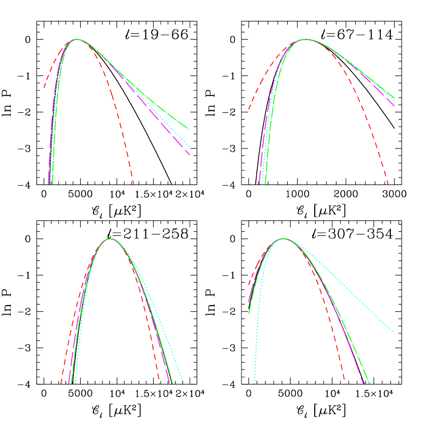
Figure 4: Full and approximate Saskatoon likelihoods. As in Fig. 2. The solid (black) line is the full likelihood calculated exactly. The short-dashed (red) line is the Gaussian approximation about the peak. The dotted (cyan) line is a Gaussian in $\ln{{\cal C}_{\ell}}$; the dashed (magenta) line is a Gaussian in $\ln{({\cal C}_{\ell}+x_{\ell})}$, as discussed in the text. The dot-dashed (green) line is the equal-variance approximation.

We have found that the shape of the power spectrum used with each bin of $\ell$ can have an impact on the likelihood function evaluated using this ansatz. Similarly, a finer binning in $\ell$ will reproduce the full likelihood more accurately. Although the maximum-likelihood amplitude at a fixed shape ($n_{s}$) does not significantly depend on binning or shape, the shape of the likelihood function along the maximum-likelihood ridge changes with finer binning and with the assumed spectral shape.

As an aside, we mention several complications that we have noted in the analysis of the Saskatoon data. Because of the complexity of the Saskatoon chopping strategy, we have found that the signal correlation matrix, $C_{T}$ is not numerically positive definite; removing the negative eigenvalues can change the value of ${\cal C}_{B}$ by as much as 5% in some bins. This should be taken as an estimate of the accuracy of our spectral determinations due to these numerical errors.

We have also found that the Fisher matrix, which we usually use as an estimate of the (inverse) error matrix for the parameters, can differ significantly from the true curvature matrix. This difference can be especially marked in low-$\ell$ bins for which the sample and/or cosmic variance can be considerable, potentially resulting in large fluctuations in this error estimate as well. In the Saskatoon plots here, we use the actual curvature matrix in place of the Fisher matrix. In a forthcoming paper (Knox & Jaffe, 1998), we will address these and other issues of implementation of the quadratic estimator for ${\cal C}_{\ell}$.

As we will see in the following, these concerns become less important when combining Saskatoon with COBE/DMR, since the results are mostly dependent on the broad-band power probed by each experiment. Moreover, we expect that these difficulties are considerably more likely in the case of chopping experiments, for which our expression for $x_{B}$, Eq. 26 is somewhat ad hoc. Most future CMB results will be for “total-power” (i.e., mapping) experiments, and the satellites MAP and Planck will be (nearly) all-sky, like COBE/DMR, for which the offset lognormal form has proven most excellent. In any case, even with present-day data, our ansatz provides a far better approximation to the full likelihood than a simple Gaussian in ${\cal C}_{\ell}$ as was used for some global analyses of current CMB data such as Lineweaver (1997); Lineweaver (1998a); Lineweaver (1998b);Lineweaver (1998c);Lineweaver & Barbosa (1998);Hancock et al. (1998)).

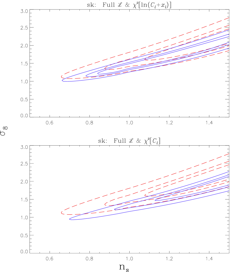
Figure 5: Likelihood contours for the Saskatoon experiment alone, as in Figure 3, but using the “orthogonalized bands” of Sec. 4.4.

6 Application to OVRO, SP and SuZIE

One of the problems we hoped to solve with better approximations to the likelihood functions than Gaussian was how to treat the valuable data with upper limits or very weak detections. In particular, the data from OVRO (Myers, Readhead & Lawrence, 1993) and SuZIE (Church et al., 1997) is useful for constraining open universe models with power spectra that do not fall off rapidly enough at high $\ell$. Although the Gaussian form does not work well here, the offset lognormal does much better and the form of Section 2.2.2 works very well, as is shown for OVRO and SP in the top panel of Fig. 6.

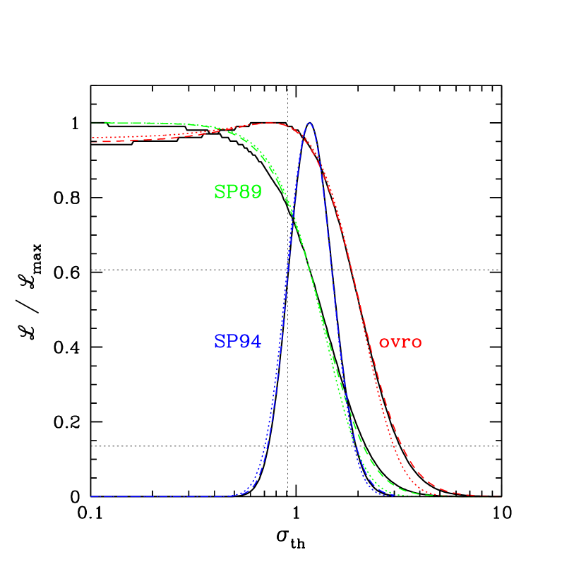
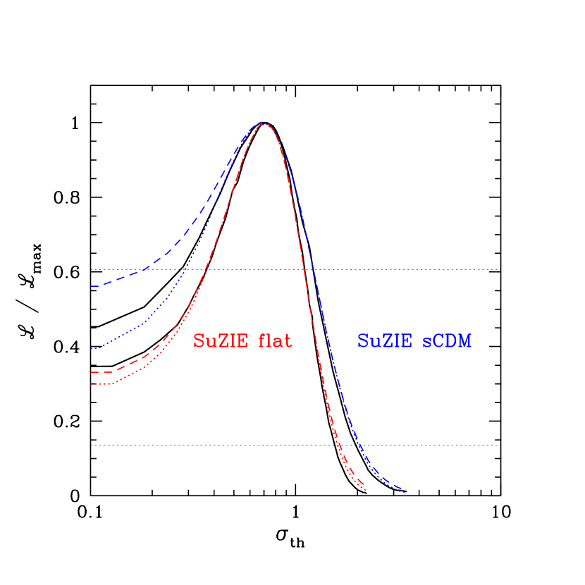
Figure 6: Upper Panel: Likelihood curves for two upper limit cases, OVRO and SP89, and SP94 which had a reasonably well determined bandpower amplitude. Lower Panel: Likelihood curves for SuZIE, using two different models for ${\cal C}_{\ell}$, sCDM and a flat bandpower. Solid (black) lines are the full likelihoods. The equal-variance approximation (dashed curve) does extremely well and the offset-lognormal (dotted curves) also does well in treating these cases. The measure of the amplitude $\sigma_{th}$ is proportional to ${\cal C}_{B}^{1/2}$. In the top panel, $\sigma_{\rm th}=\sigma_{8}$ for the untilted sCDM model; in the bottom panel, it is in units of $10^{5}\Delta T/T$.

The likelihood for the SuZIE results is also shown. The authors (Church et al., 1997) plotted the likelihood for the amplitude for several different models, which we have fit from the published figure. Although reported as an upper limit, the likelihood is peaked at positive power, but zero power is only rejected at $\sim 1\sigma$. We note as an aside that a simple flat bandpower (${\cal C}_{\ell}={\rm const}$) is not quite sufficient to contain all of the information in the SuZIE data: the likelihood function changes slightly for models with different shapes, defined as in Eq. 31—most of the physically motivated models (e.g., sCDM, $\Lambda$CDM, etc.) have roughly the same bandpower curves, but a flat bandpower gives a slightly different one as shown in the figure, and extreme open models are more similar to the flat-bandpower case than to sCDM. We also note that our equal-variance approximation performs slightly better for the flat bandpower, while the sCDM model is fit better by the offset lognormal. In any case, we again find that in all of these cases our approximations fit the likelihoods much better than any naive Gaussian approach would.

7 Results: COBE/DMR + Saskatoon

As a further example and test of these methods, we can combine the results from Saskatoon and COBE/DMR in order to determine cosmological parameters. For this example, we use the orthogonal linear combinations as described in the previous section. In Figure 7 we show the likelihood contours for standard CDM, varying the scalar slope $n_{s}$ and amplitude $\sigma_{8}$. As before, we see that the naive $\chi^{2}$ procedure is biased toward low amplitudes at fixed shape ($n_{s}$), but that our new approximation recovers the peak quite well. The full likelihood gives a global maximum at $(n_{s},\sigma_{8})=(1.15,1.67)$, and our approximation at $(1.13,1.58)$, while the naive $\chi^{2}$ finds it at $(1.21,1.55)$, outside even the three-sigma contours for the full likelihood. We can also marginalize over either parameter, in which case the full likelihood gives $n_{s}=1.17^{+0.08}_{-0.07}$, $\sigma_{8}=1.68^{+0.26}_{-0.21}$; our ansatz gives $n_{s}=1.14^{+0.07}_{-0.05}$, $\sigma_{8}=1.60\pm 0.15$; and the naive $\chi^{2}$ gives $n_{s}=1.21^{+0.08}_{-0.09}$, $\sigma_{8}=1.55^{+0.18}_{-0.20}$. (Note that even with the naive $\chi^{2}$ we marginalize by explicit integration, since the shape of the likelihood in parameter space is non-Gaussian in all cases.)

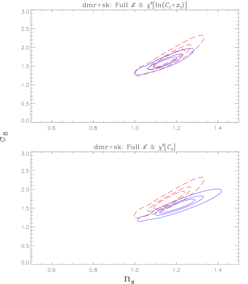
Figure 7: Likelihood contours for COBE/DMR and Saskatoon combined. As in Figure 3, but combining likelihoods from COBE/DMR and Saskatoon. For the Saskatoon calculation, we used the “orthogonalized bands” of Sec. 4.4.

8 Parameter Estimation

Above, we have discussed many different approximations to the likelihood ${\cal L}$. Here we discuss finding the parameters that maximize this likelihood (minimize the $\chi^{2}\equiv-2\ln{\cal L}$). We then apply our methods to estimating the power in discrete bins of $\ell$. This application provides another demonstration of the importance of using a better approximation to the likelihood than a Gaussian.

The likelihood functions above depend on ${{\cal C}_{\ell}}$ which may in turn depend on other parameters, $a_{p}$, which are, e.g., the physical parameters of a theory. If we write the parameters as $a_{p}+\delta a_{p}$ we can find the correction, $\delta a_{p}$, that minimizes $\chi^{2}$ by solving

$$\delta a_{p}=-\frac{1}{2}{\cal F}^{-1}_{pp^{\prime}}{\partial\chi^{2}\over\partial a_{p^{\prime}}},$$ (37)

where

$${\cal F}_{pp^{\prime}}\equiv\frac{1}{2}{\partial^{2}\chi^{2}\over\partial a_{p}\partial a_{p^{\prime}}}$$ (38)

is the curvature matrix for the parameters $a_{p}$. If the $\chi^{2}$ were quadratic (i.e., Gaussian ${\cal L}$) then Eq. 37 would be exact. Otherwise, in most cases, near enough to its minimum, $\chi^{2}$ is approximately quadratic and an iterative application of Eq. 37 converges quite rapidly. The covariance matrix for the uncertainty in the parameters is given by $\langle\delta a_{p}\delta a_{p^{\prime}}\rangle={\cal F}^{-1}_{pp^{\prime}}$. This is just an approximation to the Newton-Raphson technique for finding the root of $\partial{\cal L}/\partial a_{p}=0$; a similar techniqe is used in quadratic estimation of ${\cal C}_{\ell}$ (Tegmark, 1997; Bond, Jaffe & Knox, 1998; Oh, Spergel & Hinshaw, 1998).

As our worked example here, we parameterize the power spectrum by the power in $B=1$ to $11$ bins, ${\cal C}_{B}$. Within each of the bins, we assume ${\cal C}_{\ell}={\cal C}_{B}$ to be independent of $\ell$. We have chosen the offset lognormal approximation. The $\chi^{2}$ completely describes the model:

$$\chi^{2} = \sum_{i,j}\left(Z_{i}^{\rm t}-Z_{i}^{\rm d}\right)M_{ij}^{Z}\left(Z_{j}^{\rm t}-Z_{j}^{\rm d}\right)+\chi^{2}_{\rm cal};$$ (39)

$$\chi^{2}_{\rm cal} \equiv \sum_{\alpha}{(u_{\alpha}-1)^{2}\over\sigma_{\alpha}^{2}};$$ (40)

$$Z_{i}^{\rm d} \equiv \ln(D_{i}+x_{i});$$ (41)

$$Z_{i}^{\rm t} \equiv \ln\left(\sum_{B}u_{\alpha(i)}f_{iB}{\cal C}_{B}+x_{i}\right);$$ (42)

$$M_{ij}^{Z} \equiv M_{ij}\left(D_{i}+x_{i}\right)\left(D_{j}+x_{j}\right)\quad\mbox{no sum};$$ (43)

where $M_{ij}$ is the weight matrix for the band powers $D_{i}$. We have modeled the signal contribution to the data, $D_{i}$, as an average over the power spectrum, $\sum_{B}f_{iB}{\cal C}_{B}$, times a calibration parameter, $u_{\alpha(i)}$. For simplicity, we take the prior probability distribution for this parameter to be normally distributed. Since the datasets have already been calibrated, the mean of this distribution is at $u_{\alpha}=1$. The calibration parameter index, $\alpha$, is a function of $i$ since different power spectrum constraints from the same dataset all share the same calibration uncertainty. We solve simultaneously for the $u_{\alpha}$ and ${\cal C}_{B}$; i.e., together they form the set of parameters, $a_{p}$, in Eq. 37. For those experiments reported as band-powers together with the trace of the window function, $W^{i}_{\ell}$, the filter is taken to be

$$f_{iB}={\sum_{\ell\in B}W^{i}_{\ell}/\ell\over\sum_{\ell}W^{i}_{\ell}/\ell}.$$ (44)

Note that this is an approximation which neglects some effects of off-diagonal signal correlations (Knox, 1999).

For Saskatoon and COBE/DMR, our $D_{i}$ are themselves estimates of the power in bands. For these cases the above equation applies, but with $W_{\ell}/\ell$ set to a constant within the estimated band and zero outside. The estimated bands have different $\ell$ ranges than the target bands.

Instead of the curvature matrix of Eq. 38 we use an approximation to it that ignores a logarithmic term. Including this term can cause the curvature matrix to be non-positive definite as the iteration proceeds. The approximation has no influence on our determination of the best fit power spectrum, but does affect the error bars. We have found that the effect is quite small.

We now proceed to find the best-fit power spectrum given different assumptions about the value of $x_{i}$, binnings of the power spectrum and editings of the data. See Appendix C for a tabulation of the bandpower data we are using.

We have determined the $x_{i}$ only for COBE/DMR, Saskatoon, SP89, OVRO7, SuZIE and TOCO. (Although not included in Table 2, the highly constraining measurement near $l=400$ by TOCO98 (Miller et al., 1999) is also well-fit by the offset lognormal form.) To test the sensitivity to the unknown $x_{i}$s we found the minimum-$\chi^{2}$ power spectrum assuming the two extremes of $x_{i}=0$ (corresponding to lognormal) and $x_{i}=\infty$ (corresponding to Gaussian). These two power spectra are shown in Fig. 8. Note that both power spectra were derived using our measured $x_{i}$ values; only the unknown $x_{i}$ values were varied. The variation in the results would be much greater if we let these $x_{i}$ values be at their extremes. In what follows the unknown $x_{i}$ are set to zero.

Sometimes when the entire likelihood function is unavailable, enough information is given to allow an estimation of the $x_{i}$ for individual experiments that give single bandpower estimates. For example, we may be given $D_{m}$ where the likelihood is a maximum and $D_{\pm}$ where the likelihood has fallen by $\exp(-1/2)$, the latter giving an estimate of asymmetric 1 sigma error bars. We can then estimate the error $\sigma$ and the value of $x$ in the offset lognormal form from:

$$\sigma=\ln(s_{+}/s_{-})\,,$$

$$x=D_{m}\left[s_{+}s_{-}/(s_{+}-s_{-})-1\right]\,,$$ (45)

where

$$D_{\pm}\equiv D_{m}(1\pm s_{\pm})$$ (46)

defines $s_{\pm}$. Note that $x$ is indeterminant for $s_{+}=s_{-}$, but this Gaussian limit is approached from the large $x$ direction. It yields an error on $D-D_{m}$ of $x\sigma\rightarrow D_{m}(s_{+}+s_{-})/2$, the required Gaussian error.

Although the determination of the effective error is quite stable as $s_{-}\rightarrow s_{+}$, this is not so for $x$, where small errors in $s_{-},s_{+}$ can lead to big changes. The $x>0$ constraint implies $s_{-}s_{+}>(s_{+}-s_{-})$, which can still be violated though $s_{+}>s_{-}$. Even if this does occur, the lognormal form may still be a reasonable fit if one adjusts $x$ and $\sigma$. On the other hand, if the probability is skewed towards small amplitudes, as can happen when there is another signal such as a dust component that has been marginalized, the lognormal fit can never work.

Most often, the reason we cannot get good values of $x$ from asymmetric error bars is that the limits quoted in the literature are the Bayesian integral 16% and 84% probability ones, with an assumed prior (e.g., uniform in the bandpower amplitude). We need to know the likelihood shape to estimate $x$ from those $s_{\pm}$. (One could adopt the lognormal and fit for these integral quantities, a step we have not taken.) For example, We have found that adopting Eq. (45) leads to negative values for $x$ for Tenerife, MAX4 and MAX5 values taken from the literature.

Except for the cases noted, we always use $x$’s for the experiments where we have determined them well, those given in Table C2. When we must resort to the Eq. (45) procedure to estimate them, we usually set all $x$’s to zero if they are negative. For the positive values, we have tested the Eq. (45) $x$ values with our $x=0$ results and find that it makes little difference in the compressed bandpower results.

Our results have some sensitivity to binning, partly because the visual representation does not describe the correlation between bins. This is especially so for the last bin for which upper limits play a large role. A procedure often used to control such variations is to introduce a prior probability $P_{P}({\cal C}_{B})=\exp[S_{P}({\cal C}_{B})]$ for the ${\cal C}_{B}$. In this section, we have implicitly adopted a uniform prior, which is the least prejudiced one to adopt in that only the data decides what the bandpowers should be. However, we have also experimented with other priors, such as a Gaussian priors, with $S_{P}\propto-({\cal C}_{B}/{\cal C}_{B*}-1)^{2}/(2\sigma_{P}^{2})$ and a “maximum entropy” prior,

$$S_{P} = \alpha{\cal C}_{B*}\times$$

$$[-({\cal C}_{B}/{\cal C}_{B*})\ln({\cal C}_{B}/{\cal C}_{B*})+({\cal C}_{B}/{\cal C}_{B*}-1)].$$

Here ${\cal C}_{B*}$ is some target value, associated with an assumed prior model, $\sigma_{P}^{2}$ is an adjustable variance in the Gaussian case and $\alpha$ is an adjustable parameter in the maximum entropy case. For example, the maximum entropy prior is designed to avoid negative ${\cal C}_{B}$, relaxes to ${\cal C}_{B*}$ where there is little data and ensures some degree of smoothness in the determinations. However, especially in regions where the input shape for ${\cal C}_{B*}$ is changing rapidly (e.g., the damping tail), this procedure can give the wrong impression. Given the current state of the data, we prefer to show a few binnings to demonstrate sensitivity. When the data improves, it will be reasonable to try other priors, for example those that exert penalties if the data does not give continuity in $\ell$.

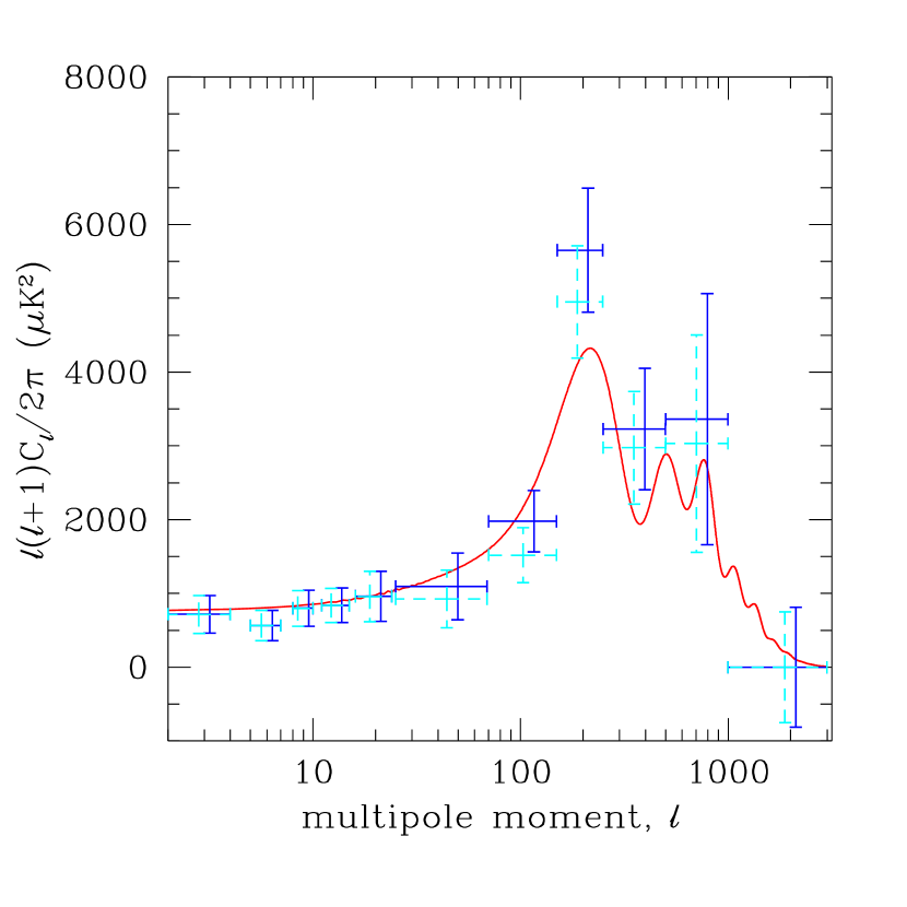
Figure 8: Power spectra that minimize the $\chi^{2}$ in Eq. 39. The solid (dashed) error bars assume $x=0$ ($x=\infty$) for those datasets with no determination of $x$; the two sets have been offset slightly for display purposes. Solid curve is standard CDM.

$\ell_{\rm min}$	$\ell_{\rm max}$	power	standard error	correlation
2	4	721	255	-0.08
5	7	566	205	-0.11
8	10	799	242	-0.08
11	15	842	233	-0.11
16	39	907	313	-0.17
40	99	1027	331	-0.32
100	169	3205	610	-0.16
170	249	6216	1040	-0.15
250	399	2394	1106	-0.62
400	999	3328	1218	-0.31
1000	2999	0.0	783

Table 1: Estimated binned power spectrum. The power and standard error are in $\mu{\rm K}^{2}$ and are the numbers corresponding to the data points in Fig. 11. The correlation column lists the correlation ($\equiv{\cal F}^{-1}_{BB^{\prime}}/\sqrt{{\cal F}^{-1}_{BB}{\cal F}^{-1}_{B^{\prime}B^{\prime}}}$) between bin $B$ and the next highest bin, $B^{\prime}=B+1$.

The $\chi^{2}$ (of Eq. 39) for the fit in Table 1 is 62 for 63 degrees of freedom. Thus the scatter of the band powers is consistent with the size of their error bars; it provides no evidence for contamination, mis-estimation of error bars, or severe non-Gaussianity in the probability distribution of the underlying signal.

In choosing a particular binning, there is a tradeoff to be made between preserving shape information and reducing both error bars and correlation. From Table 1 one can see the extent to which the bins are correlated. The nearest-neighbor bin is by far the dominant off-diagonal term. For this particular binning, all others are ten percent or less, except for the ninth bin—eleventh bin correlation which is 0.2. The lower $\ell$ bands have the smallest correlations as we would expect from DMR. There are some very strong correlations in the higher bands. Fortunately, from Fig. 9 we see that some general features are quite robust under different binnings. Namely, the spectrum is flat out to $\ell\simeq 80$ or $100$, there is a rise to $\ell\simeq 250$ or $350$ and then a drop in power beyond $\ell\simeq 350$. Although the data clearly indicate a peak, it is difficult to locate the position to better than $\pm 70$. In the top panel the rise to the Doppler peak has been binned more finely than the others. This is a particularly difficult area to resolve with current data: the correlation between the sixth and seventh bins is $-0.75$.

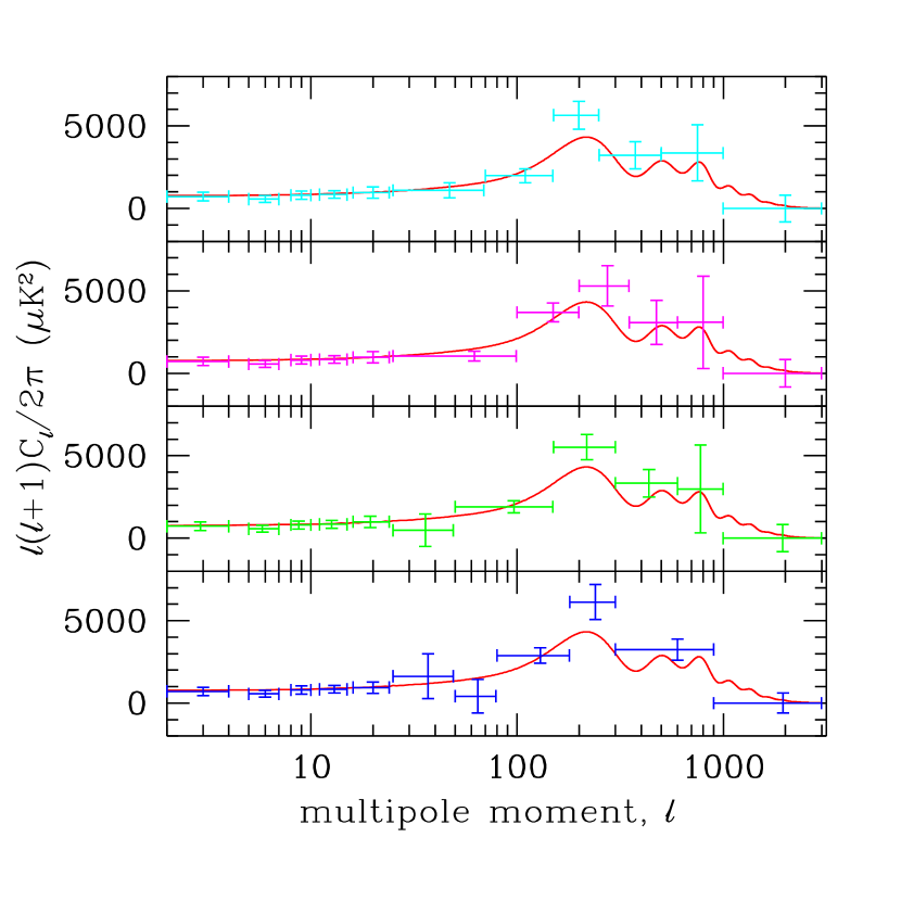
Figure 9: Power spectra that minimize the $\chi^{2}$ in Eq. 39 under different binnings. Solid curve is standard CDM.

We also see, from Figure 10, that the general picture does not depend on one single dataset—though the error bars do get significantly larger when the Saskatoon dataset is ignored. Also, if we were to ignore OVRO, the highest $\ell$ bin would have error bars larger than the graph.

Figure 10: Power spectra that minimize the $\chi^{2}$ in Eq. 39 under different editings of the data. Top panel: no TOCO. Middle panel: no MSAM, bottom panel: no Saskatoon. Solid curve is standard CDM.

The upper limits from SuZIE and OVRO constrain a region of the power spectrum otherwise unconstrained and put some pressure on models with small-scale power, such as open models. Due to the high interest in these limits, and the difficulty in interpreting the error bars in these figures (once again due to their non-Gaussianity) we have attempted to display their constraints on the spectrum in an additional, independent manner. We do so by using the published bounds on Gaussian auto-correlation functions (GACFs). The GACF is given by

$${\cal C}_{\ell}=C_{0}\ell^{2}\theta_{c}^{2}\exp\left(-{1\over 2}\ell^{2}\theta_{c}^{2}\right)$$ (48)

where $C_{0}$ is the amplitude of the real-space correlation function at zero lag and $\theta_{c}$ is called the Gaussian coherence angle. For various choices of the coherence angle, the data were used to set limits on $C_{0}$. The curves in Fig. 11 trace the peak of the GACF with $C_{0}$ at the 95% confidence upper limit as $\theta_{c}$ is varied.

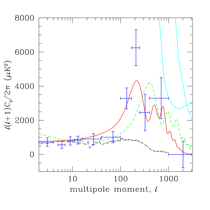
Figure 11: Binned power spectrum that minimizes the $\chi^{2}$ in Eq. 39 and which is tabulated in Table 1. In addition to the data presented in Table 2 these results also include TOCO98(Miller et al., 1999). Solid curve is standard CDM, dashed curve is an open CDM model with matter density one third of critical, baryon mass density of 0.035 times critical and a Hubble constant of 60 km/sec/Mpc. The dotted curve is a prediction for local cosmic strings (Allen et al., 1997). Curves at high $\ell$ indicate upper limits derived from OVRO (left) and SuZIE (right) data.

As we have emphasized earlier with the band-powers, it can often be misleading to interpret the covariance matrix of the parameters (derived from the Fisher matrix) as indicating the 68% confidence region, since the 68% confidence region may extend beyond the region of validity for the quadratic approximation to $\chi^{2}$. Even in such a case though, the quadratic procedure still may be useful just for finding the minimum, which might be a good point to begin further investigation of the $\chi^{2}$ surface without the quadratic approximation. Non-Gaussianity can be especially severe when the parameters are cosmological parameters.

9 Summary and Discussion

We have argued that cosmological parameters should be constrained from CMB datasets via an initial step of determining constraints on the power spectrum. These power spectrum constraints can themselves be viewed as a compressed version of the pixelized data. We call this process radical compression since the resulting dataset is orders of magnitude smaller than the original. One must be careful in using this compressed data to take into account the non-Gaussian nature of their probability distributions; ignoring the non-Gaussianity while attempting to constrain parameters results in a bias. The offset lognormal and equal variance approximations capture its salient characteristics. They are both specified by the mode, variance and the noise contribution to the variance ($x$). Use of these forms allows for a very simple $\chi^{2}$ type treatment of the band-power data—without the bias.

While we have found these approximations to the likelihood functions to be quite adequate for dealing with the data we have explored to date, and have given quite general arguments for why the tails behave as they do, our checks have not been exhaustive. For example, some quoted CMB anisotropy results are skewed to lower rather than higher amplitudes (perhaps due to fitting out foregrounds or systematics), a situation that the offset lognormal cannot fit. Just as one computes the curvature about the maximum likelihood, so one can consider computing a skewness that would encapsulate such behavior, but we will leave the search for further likelihood function approximations to further exploration.

We have shown that the offset lognormal approximation applied to a two-parameter ($\sigma_{8}$ and $n_{s}$) family of CDM models works very well. We have also used this form to find the maximum-likelihood binned power spectrum, given the band-power data. The resulting graphs provide a visual representation of the power spectrum constraints that is, in our opinion, far superior to plotting all the band-power data on top of each other.

The exercise of estimating the binned power spectrum immediately raises the question of how well it would work to estimate cosmological parameters using these as a “super-radically compressed dataset”. We plan to pursue this question in future work.

Although our examples have focused on using our approximations in order to derive parameter constraints from more than one dataset, we believe they may also prove useful for estimating cosmological parameters from single, very powerful datasets, such as those that are expected to come from a number of experiments over the next decade. We must note though that once a dataset has sufficient “spectral resolving power” and dynamic range there is another approach that can be used to remove the cosmic bias. This alternative approach was suggested in Bond, Jaffe & Knox (1998) and Seljak (1997) and successfully applied to simulated MAP data in Oh, Spergel & Hinshaw (1998). The idea is to exploit the fact that we expect there to be no fine features in the CMB power spectrum and therefore use some smoothed version of the estimated power spectrum to calculate the Fisher matrix. Heuristically one expects this to remove the bias, since upward-fluctuating points no longer receive less weight than downward-fluctuating points. Although this smoothing technique is quite likely to be successful, we point out that, unlike our ansatz, it relies on an assumption of the smoothness of the power spectrum.

One of our main objectives with this paper is to provide observers with a method for presenting their results that will allow efficient combination with the results of others in order to create a joint determination of cosmological parameters. The method is fully described in Appendix B. In this appendix we also discuss complications due to overlapping sky coverage and upper limits.

Appendix A Signal-to-Noise Eigenmodes and the general form of the likelihood

We start with the full-sky likelihood, either in the form of Eq. 2.2.1 or in terms of $Z=\ln({\cal C}+x)$, Eq. 17. We transform this form to signal-to-noise eigenmodes (e.g., Bond (1994);Bunn & White (1997);Bond, Jaffe & Knox (1998)). Here, the data in the signal-to-noise eigenmode basis are $d_{k}$, with diagonal covariance,

$$\langle d_{k}d_{k^{\prime}}\rangle=(1+\sigma^{2}_{\rm th}\lambda_{k})\delta_{kk^{\prime}}.$$ (A1)

We allow the amplitude, $\sigma^{2}_{\rm th}$, for the signal contribution to vary, since the eigenmodes only depends upon the shape of the signal covariance, itself dependent on the input power spectrum. If we define the signal-to-noise transformation with power spectrum ${\cal C}_{\ell}^{\rm shape}$, then Eq. A1 is valid for all ${\cal C}_{\ell}=\sigma^{2}_{\rm th}{\cal C}_{\ell}^{\rm shape}$. The eigenvalue for mode $k$ is $\sigma_{\rm th}^{2}\lambda_{k}$, with units of (signal-to-noise)².

Because the Gaussian variables, $d_{k}$, are statistically independent, the likelihood is made up of independent contributions,

$$\ln{\cal L}/{\widehat{\cal L}} = -{{1\over 2}}\sum_{k}\bigg{[}{d_{k}^{2}\over 1+{\widehat{\sigma}^{2}_{\rm th}}\lambda_{k}}{({\widehat{\sigma}^{2}_{\rm th}}-\sigma^{2}_{\rm th})\lambda_{k}\over 1+\sigma^{2}_{\rm th}\lambda_{k}}$$ (A2)

$$\quad+\ln{1+\sigma^{2}_{\rm th}\lambda_{k}\over 1+{\widehat{\sigma}^{2}_{\rm th}}\lambda_{k}}\bigg{]}\,,$$

where a “hat” refers to the quantity at the likelihood maximum.

Introducing the number of modes with a given value of $\lambda$, $g(\lambda)$, and the cumulative number of modes $G(\lambda)=\sum_{\lambda^{\prime}>\lambda}g(\lambda^{\prime})$, this can be written in the suggestive form

$$\ln{\cal L}/{\widehat{\cal L}} = -{1\over 2}\int dG(\lambda)\bigg{[}\left[Z(\lambda)-{\widehat{Z}}(\lambda)\right]$$ (A3)

$$+{\chi^{2}_{\lambda}\over 1+{\widehat{\sigma}^{2}_{\rm th}}\lambda}\left(e^{-\left[Z(\lambda)-{\widehat{Z}}(\lambda)\right]}-1\right)\bigg{]}\,.$$

Here $\chi^{2}_{\lambda}=\sum_{\lambda_{k}=\lambda}d_{k}^{2}/g(\lambda)$ is the $\chi^{2}$ per degree of freedom for modes of the $\lambda$. On average, $\chi^{2}_{\lambda}$ approaches $(1+{\widehat{\sigma}^{2}_{\rm th}}\lambda)$, in which case the form is a sum of terms like Eq. 16. The variables $Z(\lambda)\equiv\ln(1+\sigma^{2}_{\rm th}\lambda)$ are analogous to the form we have been using if $\lambda^{-1}$ is interpreted as a special case of the offset $x$. The integral is to be interpreted in the Stieltjes sense, as a sum over the discrete $\lambda$ spectrum, $\sum_{\lambda}g(\lambda)(\ldots)$.

Consider what happens asymptotically with increasing $\sigma^{2}_{\rm th}$. The modes with $\sigma^{2}_{\rm th}\lambda>1$ contribute, so $G(\sigma_{\rm th}^{-2})\ln\sigma^{2}_{\rm th}$ is the leading behavior. As $\sigma^{2}_{\rm th}$ goes up, more eigenmodes may contribute, $\ln{\cal L}/{\widehat{\cal L}}$ decreases faster, modifying the tail.

Appendix B Data Reporting Recipe

We recommend reporting future (and, if possible, past) CMB results in a form that will render them amenable to this “radically-compressed” analysis. Thus, experimenters and phenomenologists ought to provide estimates of

• ${\cal C}_{\ell}\equiv\ell(\ell+1)C_{\ell}/(2\pi)$, the power spectrum in appropriate bins;

• ${\cal F}^{-1}_{\ell\ell^{\prime}}$, the curvature or covariance matrix of the power spectrum estimates; and

• $x_{\ell}$, the quantity such that $Z_{\ell}\equiv\ln({\cal C}_{\ell}+x_{\ell})$ is approximately distributed as a Gaussian.

We here provide an outline of the steps needed to provide the appropriate information. Current listings of publicly-available results will be posted at http://www.cita.utoronto.ca/$\sim$knox/radical.html. Please contact the authors to have results included.

1) Divide the power spectrum into discrete bins. To prevent significant loss of shape information, the bins should not be too large. However, there may be a problem with making the bins too small. The closer we are to the case of well-determined, independent bins, the better our ansatz is expected to work. Thus bins should be large enough to keep relative error bars smaller than 100% and bin to bin correlations small. The shape-dependence resulting from coarse bins can be reduced by the use of a filter function for each band (see Knox (1999)), as was done with the MSAM (Medium Scale Anisotropy Measurement) three-year data (Wilson et al., 1999).
2) Find the power in each bin that maximizes the likelihood and evaluate the curvature matrix at this point. This can be done using your favorite likelihood search algorithm. For COBE/DMR and Saskatoon we have used the iterative scheme described in Bond, Jaffe & Knox (1998). Our current implementation does not include a transformation to S/N-eigenmode space. In a forthcoming paper (Knox & Jaffe, 1998), we will provide detailed information on the implementation of this quadratic estimator and an appropriate sample set of programs.
3) Estimate $x$ for each of the bins. If the likelihood is calculated explicitly, this can simply be done by numerical fitting to the functional form of our ansatz, Eqs. 8 and following, or Eq. 34. If the likelihood peak is determined by the iterative quadratic scheme or some other method which also calculates the curvature matrix (or, less-preferably, Fisher matrix), the appropriate formulae from Sec. 2.2 (for total-power mapping experiments) or Sec. 4.1 (Eq. 28 for chopping experiments).
4) Do not alter the curvature matrix by folding in the calibration uncertainty in any way. Report the calibration uncertainty separately.

B.1 Special Cases

1) Overlapping sky coverage. Power spectrum constraints will be correlated if they are from datasets with overlapping sky coverage and sensitivity to similar angular scales. We have no general theory of these correlations. Proper combination of overlapping datasets appears to require a joint likelihood analysis to produce their combined constraints on the power spectrum.

2) Upper Limits. For datasets that can only provide an upper limit to the power spectrum amplitude, a simple option would be to calculate the full likelihood directly and simply fit to one of the two forms for ${\cal C}_{\ell}\geq 0$ but with a negative or very small ${\cal C}_{\ell}$ (and such that ${\cal C}_{\ell}+x_{\ell}>0$). This is what we have done for Fig. 6 which demonstrates that both of our approximate forms work fairly well, especially the full form of Section 2.2.2.

Although the results in Fig. 6 look quite impressive, they say nothing about how well the window function tells us which regions of the power spectrum are being constrained by the data. In other words, does the trace of the window function make a good filter function? Therefore, we present the following alternative method for reporting upper limits which includes a prescription for creation of a filter function.

The data can be reported as amplitudes of signal-to-noise eigenmodes and their eigenvalues (see Appendix A). One need only report the modes with the largest eigenvalues. The number of modes that it is necessary to report is likely to be quite small. The likelihood of $\sigma^{2}_{\rm th}$, where ${\cal C}_{\ell}=\sigma^{2}_{\rm th}{\cal C}_{\ell}^{\rm shape}$, is then:

$$\chi^{2}\equiv-2\ln{\cal L}=\sum_{i}\left[\ln\left(1+\sigma^{2}_{\rm th}\lambda_{i}\right)+{D_{i}^{2}\over 1+\sigma^{2}_{\rm th}\lambda_{i}}\right]$$ (B1)

where $D_{i}$ is the amplitude of the $i$th mode, $\lambda_{i}$ is its eigenvalue, and ${\cal C}_{\ell}^{\rm shape}$ is the power spectrum used to define the S/N-modes. Of course, we want the likelihood to be a function of, e.g., a binned power spectrum. It is, via:

$$\sigma^{2}_{\rm th}={1\over{\cal C}}\sum_{B}f_{B}{\cal C}_{B}$$ (B2)

where we have assumed a flat power spectrum (${\cal C}_{\ell}^{\rm shape}={\cal C}={\rm const}$), $f_{B}$ is related to the window function as in Eq. 44 or, better, derived from the Fisher matrix as described in Bond, Jaffe & Knox (1998). It is straightforward to calculate the derivatives of this $\chi^{2}$ with respect to ${\cal C}_{B}$ in order to combine upper limits with detections and perform the search procedure described in Section 8.

Appendix C Band Powers

Table 2: Input band powers, standard errors, and noise contributions to the variance ($x$) in $\mu{\rm K}^{2}$.

dataset	$\ell_{\rm-}$–$\ell_{\rm+}$	BP	err	$x$	reference
firs	4–25	927.8	440.7	??	Ganga et al. (1994); Bond (1994)
tenerife595	13–28	1164	705.9	??
BAM	31–90	870.3	478.5	??	Tucker et al. (1997)
SP91-6225-63	35–98	892.2	382.8	??	Gaier et al. (1991); Schuster et al. (1991)
SP94-62-4ch	33–95	837.5	384.6	??	Gundersen et al. (1995)
SP94-62-3ch	40–114	1632	584.5	??	Gundersen et al. (1995)
pyth96I-II-III	52–99	2916	1351	??	Platt et al. (1997); Ruhl et al. (1995)
pyth96III	132–237	3364	1565	??	Platt et al. (1997); Ruhl et al. (1995)
qmap_q	79–143	2704	520.0	??
qmap_ka1	60–101	2209	604.5	??
qmap_ka2	99–153	3481	760.5	??
toco97_3	45–81	1600	720	500	Torbet et al. (1999)
toco97_4	70–108	2040	600	100	Torbet et al. (1999)
toco97_5	90–138	4900	850	0	Torbet et al. (1999)
toco97_6	135–180	7850	1300	0	Torbet et al. (1999)
toco97_7	170–237	7170	1300	3000	Torbet et al. (1999)
sp89	87–247	0.0	1459	1830	Meinhold & Lubin (1989)
argo	69–144	1060	613.0	??	Masi et al. (1996); DeBernardis et al. (1994)
MAX4av	89–249	2586	876.9	??	Clapp et al. (1994); Devlin et al. (1994)
MAX5av	89–249	1511	573.8	??	Lim et al. (1996); Lim et al. (1996)
ovro22	362–759	3127	813.1	??	Leitch (1998)
cat1	349–473	2583	1512	??	Scott et al. (1996)
cat2	559–709	2401	1584	??	Scott et al. (1996)
cat1-98	349–473	3937	2322	15700	Baker et al. (1998)
cat2-98	559–709	0.0	5031	15700	Baker et al. (1998)
OVRO	1147–2425	72.4	380.3	367	Myers, Readhead & Lawrence (1993)
SuZIE	1366–3000	354.3	753.4	122	Church et al. (1997)

Note. — These data, their window functions, and also data for MSAM-3yr (Wilson et al., 1999), Saskatoon (Netterfield et al., 1997) and COBE/DMR (Bennett et al., 1996) are available at http://www.cita.utoronto.ca/$\sim$knox/radical.html. These last three datasets are not shown in the table here because they have multiple bands with covariance matrices.

The numbers in Table 2 were used to form part of the weight matrix in Eq. 39: $W_{ij}=1/\sigma_{i}^{2}\delta_{ij}$ where $\sigma_{i}$ is from the “standard error” column of the Table. These standard errors are derived from published likelihood maxima ($D_{i}$), 68% confidence upper limits ($D_{i}^{u}$) and lower limits ($D_{i}^{l}$). Since the upward and downward excursions from the mode to the upper and lower limits are usually different, there is some freedom in assigning a single standard error. We define $\sigma_{i}$ as an average of these excursions:

$$\sigma_{i}=\left[\left(D_{i}^{u}-D_{i}\right)+\left(D_{i}-D_{i}^{l}\right)\right]/2.$$ (C1)

If the published number is linear instead of quadratic, then $D_{i}=\delta T_{i}^{2}$, etc.  and the above equation still applies. We have also tried producing $\sigma_{i}$ from averaging the inverse square of the upward and downward deviations, and found no significant difference in the results (power in bands changes by less than 10% of the error bar).

We also found not much difference in the results depending on how we treated calibration uncertainty. Most experiments report their upper and lower limits with calibration uncertainty included. Only for Saskatoon, MSAM, QMAP, TOCO97 and TOCO98 have we included calibration uncertainty by treating it as an independent parameter ($u_{\alpha}$ in Eq. 39).

Missing from the table are detections from the White Dish (Tucker et al., 1993) experiment. The White Dish dataset was compressed to two band-power detections with sensitivity in the range $\ell\sim 300$ to $\sim 600$. A recent reanalysis (Ratra et al., 1997), results in upper limits which are sufficiently loose that including them would make no difference in our power spectrum determination. Both these analyses use only a small subset of the available data; a complete analysis will probably provide detections (Griffin et al., 1998).

References

- Bond, Efstathiou & Tegmark (1997) Bond, J.R., Efstathiou, G., and Tegmark, M. 1997, MNRAS, 291, L33.
- Allen et al. (1997) Allen, B. et al.1997, Phys. Rev. Lett., 79, 2624
- Baker et al. (1998) Baker, J.C. et al.1998, MNRAS, submitted.
- Bartlett et al. (1999) Bartlett, J.G., Douspis, M., Blanchard, A., Le Dour, M., 1999, A&A, submitted. astro-ph/9903045.
- Bennett et al. (1996) Bennett, C.L., Banday, A.J., K.M. Gorski, Hinshaw, G., Jackson, P.D., Keegstra, P., Kogut, A., Smoot, G.F., Wilkinson, D., and Wright, E.L. 1996, ApJ, 464, L1, and 4-year COBE/DMR references therein.
- Bond (1994) Bond, J.R. 1994, Phys. Rev. Lett., 74, 4369.
- Bond & Jaffe (1998a) Bond, J.R. and Jaffe, A.H. 1998a, in Microwave Background Anisotropies, Proceedings of the XVI Rencontre de Moriond, ed. Bouchet, F.R. (Paris: Editions Frontieres).
- Bond & Jaffe (1998b) Bond, J.R. and Jaffe, A.H. 1998b, Phil. Trans. R. Soc. Lond. A, to appear.
- Bond, Jaffe & Knox (1998) Bond, J.R., Jaffe, A.H. and Knox, L.E. 1998, Phys. Rev. D, in press; astro-ph/9708203.
- Bond, Pogosyan & Souradeep (1998) Bond, J.R., Pogosyan, D., and Souradeep, T. 1998, Class. Quant. Gravity, in press.
- Bunn & Sugiyama (1995) Bunn, E.F. and Sugiyama, N. 1995, ApJ, 446, 49.
- Bunn & White (1997) Bunn, E.F. and White, M. 1997, ApJ, 480, 6.
- Cheng et al. (1994) Cheng, E.S. et al.1994, ApJ, 422, L37.
- Cheng et al. (1997) Cheng, E.S. et al.1997, ApJ, 488, L59.
- Church et al. (1997) Church, S.E. et al.1997, ApJ, 4 84, 523.
- Clapp et al. (1994) Clapp, A.C. et al.1994, ApJ, 433, L57.
- DeBernardis et al. (1994) DeBernardis, P. et al.1994, ApJ, 422, L33.
- de Oliveira-Costa et al. (1998) de Oliveira-Costa, A. et al.1998, astro-ph/9808045.
- Devlin et al. (1994) Devlin, M.J. et al.1994, ApJ, 430, L1.
- Devlin et al. (1998) Devlin, M. et al.1998, astro-ph/9808043.
- Efstathiou et al. (1998) Efstathiou, G., Bridle, S.L., Lasenby, A.N., Hobson, M.P. and Ellis, R.S. 1997, MNRAS, submitted.
- Ferreira, Magueijo & Gorski (1998) Ferreira, P.G., Magueijo, J., and Gorski, K.M. 1998, ApJ, accepted; astro-ph/9803256.
- Gaier et al. (1991) Gaier, T. et al.1992, ApJ, 398, L1.
- Ganga et al. (1994) Ganga, K., Page, L., Cheng, E.S., Meyer, S.S. 1994, ApJ, 432, L15.
- Griffin et al. (1998) Griffin, G.S., Nguyên, H.T., Peterson, J.B., and Tucker, G.S. 1998, in preparation.
- Guitteriez de la Cruz et al. (1995) Gutteriez de la Cruz, S.M. et al., ApJ, 442, 10.
- Gundersen et al. (1993) Gundersen, J.O. et al.1993, ApJ, 413, L1.
- Gundersen et al. (1995) Gundersen, J.O. et al.1995, ApJ, 443, L57.
- Hamilton (1997a) Hamilton, A.J.S. 1997a, astro-ph/9701008.
- Hamilton (1997b) Hamilton, A.J.S. 1997b, astro-ph/9701009.
- Hancock et al. (1998) Hancock, S., Rocha, G., Lasenby, A.N., and Gutierrez, C.M. 1998, MNRAS, 294, L1.
- Hancock et al. (1994) Hancock, S. et al.1994, Nature, 367, 333.
- Herbig et al. (1998) Herbig, T. et al.1998, astro-ph/9808044.
- Hobson & Magueijo (1996) Hobson, M.P. and Magueijo, J. 1996, MNRAS, 283, 1133.
- Jaffe, Knox & Bond (1998) Jaffe, A.H., Knox, L., and Bond, J.R. 1998, in Proceedings of the Eighteenth Texas Symposium on Relativistic Astrophysics, ed. Frieman, J., Olinto, A., and Schramm, D., in press.
- Jungman et al. (1996) Jungman, G., Kamionkowski, M., Kosowsky, A., and Spergel, D.N. 1996, Phys. Rev. Lett., 76, 1007.
- Kneissel & Smoot (1993) Kneissl, R. and Smoot, G. 1993, COBE note 5053.
- Knox (1999) Knox, L. 1999, Phys. Rev. D, in press.
- Knox (1995) Knox, L. 1995, Phys. Rev. D, 52, 4307.
- Knox & Jaffe (1998) Knox, L.E. and Jaffe, A.H. 1998, in preparation.
- Leitch (1998) Leitch, E. 1998, Caltech PhD. thesis.
- Lim et al. (1996) Lim, M.A. et al.1996, ApJ, 469, L69.
- Lineweaver (1997) Lineweaver, C.H. 1997, astro-ph/9702042.
- Lineweaver (1998a) Lineweaver, C.H. 1998a, ApJ, submitted; astro-ph/9805326.
- Lineweaver (1998b) Lineweaver, C.H. 1998b, astro-ph/9803100.
- Lineweaver (1998c) Lineweaver, C.H. 1998c, astro-ph/9801029.
- Lineweaver & Barbosa (1998) Lineweaver, C.H. and Barbosa, D. 1998, ApJ, 496.
- Lineweaver & Smoot (1993) Lineweaver, C. and Smoot, G. 1993, COBE note 5051.
- Masi et al. (1996) Masi, S. et al.1996, ApJ, 463, L47.
- Meinhold & Lubin (1989) Meinhold, P. and Lubin, P. 1989, ApJ, 370, L11.
- Miller et al. (1999) Miller, A.D.et al.1999, ApJ, astro-ph/9906421.
- Myers, Readhead & Lawrence (1993) Myers, S.T., Readhead, A.C.S., and Lawrence, C.R. 1993, ApJ, 405, 8.
- Netterfield et al. (1997) Netterfield, C.B., Devlin, M.J., Jarosik, N., Page, L., and Wollack, E.J. 1997, ApJ, 474, 47.
- Oh, Spergel & Hinshaw (1998) Oh, S.P., Spergel, D.N., and Hinshaw, G. 1998, astro-ph/9805339.
- Platt et al. (1997) Platt, S.R., Kovac, J., Dragovan, M., Peterson, J.B., and Ruhl, J.E. 1997, ApJ, 475, L1.
- Ratra et al. (1997) Ratra, B. et al.1997, astro-ph/9710270.
- Ruhl et al. (1995) Ruhl, J.E. et al.1995, ApJ, 453, L1.
- Schuster et al. (1991) Schuster, J. et al.1993, ApJ, 412, L47.
- Scott et al. (1996) Scott, P.F.S. et al.1996, ApJ, 461, L1.
- Seljak (1997) Seljak, U. 1997, astro-ph/9710269.
- Tanaka et al. (1996) Tanaka, S.T. et al.1996, ApJ, 468, L81.
- Tegmark (1997) Tegmark, M. 1997, Phys. Rev. D, 55, 5895; astro-ph/9611174.
- Tegmark (1998) Tegmark, M. 1999, ApJ, 514, L69.
- Tegmark & Hamilton (1998) Tegmark, M. and Hamilton, A. 1998, in Proceedings of the Eighteenth Texas Symposium on Relativistic Astrophysics, ed. Frieman, J., Olinto, A., and Schramm, D., in press.
- Tegmark, Taylor & Heavens (1997) Tegmark, M., Taylor, A., and Heavens, A. 1997, ApJ, 480, 22.
- Torbet et al. (1999) Torbet, E. et al.1999, astro-ph/9905100.
- Tucker et al. (1993) Tucker, G.S., Griffin, G.S., Nguyên, H.T., and Peterson, J.B. 1993, ApJ, 419, L45.
- Tucker et al. (1997) Tucker, G.S., Gush, H.P., Halpern, M., Shinkoda, I., and Towlson, W. 1997, ApJ, 475, L73.
- Watson et al. (1992) Watson, R. et al.1992, Nature, 357 660.
- Wilson et al. (1999) Wilson, G. et al.1999, astro-ph/9902047.
- Wollack et al. (1997) Wollack, E.J., Devlin, M.J., Jarosik, N., Netterfield, C.B., Page, L., and Wilkinson, D. 1997, ApJ, 476, 440.