The radio luminosity density of star-burst galaxies and co-moving star formation rate

Abstract

We present a new determination of the co-moving star formation density at redshifts $z\stackrel{{\scriptstyle<}}{{{}_{\sim}}}0.35$ from the $1.4$ GHz luminosity function of sub-mJy star-burst galaxies. Our sample, taken from Benn et al. (1993), is insensitive to dust obscuration. The shape of the Luminosity function of this sample is indistinguishable from a number of reasonable a prior models of the luminosity function. Using these shapes we calculate the modest corrections (typically $\stackrel{{\scriptstyle<}}{{{}_{\sim}}}20$ per cent) to the observed $1.4$ GHz luminosity density. We find that the cosmic variance in our estimate of this luminosity density is large. We find a luminosity density in broad agreement with that from the RSA sample by Condon et al. (1987). We infer a co-moving star formation rate surprisingly similar to coeval estimates from the Canada-France Redshift Survey, in both ultraviolet and H$\alpha$, although the later may also be affected by Cosmic variance. We conclude that the intermediate $0.05<z<0.3$ star-formation rate is not yet well determined partially due to uncertain extinction corrections, but also partially due to cosmic variance. We suggest that deep moderate area radio surveys will improve this situation considerably.

1 Introduction

In recent years a major focus of extra-galactic astrophysics has been in estimating the evolving, volume-averaged star formation rate. This work has been particularly stimulated by major advances in our ability to identify star forming galaxies at high redshifts with optical colour techniques (see e.g. Pettini et al 1998 and references therein). Early indications from comparisons of such populations in the Hubble Deep Field with similar populations at lower redshift suggested that there may have been a peak in star formation activity at a redshift of $z\sim 2$ (Madau et al 1996).

The theoretical interest in such measurements is high, partly because the integrated star formation is the major uncertainty in evolutionary models used to explain (amongst other things) the local chemical enrichment in our own galaxy, but also because models of galaxy formation based on e.g. hierarchically clustering scenarios can now make specific predictions for the integrated star formation rate at different epochs (e.g. Pei & Fall, Baugh et al 1997).

A variety of techniques have been employed to estimate the star formation rate at a number of epochs. The common feature of such techniques is to identify a tracer of star formation activity and integrate this over volume, correcting for contributions missed through sensitivity limits, obscuration or other incompleteness effects. Tracers that have been employed, include: the B-band-luminosity (Lilly et al.) U-band luminosity (Madau et al 1996), the $H\alpha$ luminosity (Kennicutt 1983), the mid-IR luminosity (Rowan-Robinson et al 1997). The optical tracers are potentially significantly affected by dust-obscuration and the corrections for this are uncertain and may be redshift dependent. In contrast Mid and Far-IR luminosity traces the star formation rate in obscured regions only. The obscured fraction itself is hotly debated. For example, de-reddening of optical-UV spectra does not guarantee an unbiased star formation rate, since the most heavily obscured and potentially dominant star forming regions may be wholly undetected in the UV.

In this paper we present the first estimate of the co-moving star formation density using as a tracer the radio luminosity of star forming galaxies. The radio luminosity traces the supernovae associated with star formation regions, and is not significantly affected by dust obscuration.

The paper is organised as follows. In the first section we describe our choice of radio sample. In the second we describe our estimation of the radio-luminosity density including corrections for incompleteness. In the third section we describe the conversion from luminosity density into star formation rate. In the final section we discuss our estimation of the star formation rate in the context of other determinations and other implications.

2 The 1.4GHz Sample

Deep 1.4 GHz radio source counts obtained in the last decade (Condon & Mitchell 1984; Windhorst 1984; Windhorst et al. 1985) show a steepening below a few mJy. This excess of faint sources relative to the Euclidean value can neither be attributed to the giant ellipticals and quasars responsible of most of the counts observed at fluxes $>5$ mJy, nor to the non-evolving population of normal spiral and Seyfert galaxies. Optical identification works published so far have shown that the sub–mJy sources are mainly identified with faint blue galaxies (Kron, Koo & Windhorst 1985; Thuan & Condon 1987), often showing peculiar optical morphologies indicative of interaction and merging phenomena and spectra similar to those of the star–forming galaxies detected by IRAS (Benn et al. 1993, B93). Although all these works are based on very small percentages of identification (due to the fact that the majority of the faint radio sources have very faint optical counterparts), they all agree that most of the sub–mJy radio sources with identifications brighter than $B\simeq 22-22.5$ are star–forming galaxies. In contrast, recent extensions to fainter optical magnitudes show strong hints of an increase in the fraction of early–type galaxies among the identifications of sub–mJy sources ($S_{1.4~{}GHz}\geq 0.2$ mJy; Gruppioni et al. 1998, in preparation). Thus, down to optical magnitudes of $B\sim 22.5$ most (or eventually all) of the star-burst counterparts of sub–mJy sources brighter than $S_{1.4~{}GHz}\sim 0.1-0.2$ mJy should be detected.

The B93 identification sample consists of 112 candidate optical counterparts of $\sim 500$ sub–mJy radio sources drawn from the three largest deep 1.4 GHz radio surveys (0852$+$17 field, Condon & Mitchell 1984; 1300$+$30 field, Mitchell & Condon 1985; 0846$+$45 field, Oort 1987). All the selected sources have radio fluxes greater than 0.1 mJy and optical counterparts brighter than $V=20.0$ (0846$+$45 field), $B=21.4$ (0852$+$17 field) and $B=22.3$ (1300$+$30 field). The radio flux limit varies across the survey and the areal coverage ($\Omega(S)$) of the B93 sample is a complicated function of radio flux, which is plotted in Figure 1. Spectra have been obtained for 87 of these, providing object type and spectroscopic redshifts, though at $z>0.35$ H$\alpha$ is unobservable in their spectra so the spectroscopy is only complete at low redshifts. Of these sources with spectra, 47 turned out to be star-burst galaxies. The B93 sample is the largest spectroscopic sample of sub–mJy sources so far available in literature and, due to its radio and optical limits, is the most complete sample of radio–selected sub–mJy star–forming galaxies. This sample is therefore the best currently available and is the most suitable for estimating the star–formation history as traced by the radio luminosity density of star forming galaxies.

In all the following analysis we use only those objects within B93 which Rowan-Robinson et al. identified as star-burst galaxies.

Figure 1: The areal coverage $\Omega(S)$ of the B93 sample as a function of 1.4 GHz flux limit

3 The luminosity function and luminosity density

3.1 Basic Method

To calculate both the luminosity function and the luminosity density we require an estimate of the effective volume within which each object of the sample could have been observed. Besides a $z\leq 0.35$ spectroscopic redshift limit, the B93 sample has two flux limits, one radio and one optical, this effective volume is thus given by the following expression

$$V_{i}=\int_{0}^{\infty}P({\cal O}|L_{i},L_{B,i},z)\Omega_{\rm max}\frac{dV}{dz}dz$$ (1)

where $P({\cal O}|L,L_{B},z)$ is the probability of observing an object of radio luminosity $L$ and optical luminosity $L_{B}$ at redshift $z$ within our survey, given by

$$P({\cal O}|L_{i},L_{B,i},z)=\sum\frac{\Omega(S(L_{i},z))}{\Omega_{\rm max}}P({\cal O}|S_{B}),$$ (2)

where the summation is over each of the three survey areas, in our case $P({\cal O}|S_{B})$ is either 1 or 0 depending on whether the magnitude is below or above the limit in that survey area. The radio fluxes are calculated assuming a radio spectral index, $\alpha=d\log(S_{\nu})/d\log(\nu)=0.8$; the optical fluxes are calculated using the $K$-corrections for Scd galaxies given by Metcalfe et al. (1991) and we assume a cosmology of $\Omega_{0}=1$, $\Omega_{\Lambda}=0$, $H_{0}=50h_{50}$ km s^-1 Mpc^-1 throughout.

Having determined $V_{i}$ we can use the estimator $\varphi(L)=\sum 1/V_{i}$ (Schmidt 1968), and likewise estimate the luminosity density by $\Phi_{1.4}=\sum L_{i}/V_{i}$. In the absence of luminosity cuts these estimators are unbiased, however one might worry about using these estimators to determine the radio luminosity function and luminosity density if the optical flux cut was much more severe than the radio, leading to poor sampling of the radio luminosity plane. We will demonstrate that this is not the case.

In the presence of luminosity cuts, introduced for example by redshift cuts these estimators need to be modified thus:

$$\Phi_{1.4}=\frac{1}{C({L_{\rm min},L_{B,{\rm min}}})}\sum\frac{L_{i}}{V_{i}}$$ (3)

where $C({L_{\rm min},L_{B,{\rm min}}})$ is a measure of the “completeness” of the sample being the fraction of luminosity density above the minimum observable radio and optical luminosities i.e.

$$C=\frac{\int_{L_{\rm min}}^{+\infty}\int_{L_{B,{\rm min}}}^{+\infty}L\varphi(L,L_{B})d\log L_{B}d\log L}{\int_{-\infty}^{+\infty}\int_{-\infty}^{+\infty}L\varphi(L,L_{B})d\log L_{B}d\log L}.$$ (4)

$\varphi(L,L_{B})$ is the 1.4 GHz optical bi-variate luminosity function.

We will show that these correction factors are principally determined by the shape of the luminosity function. Maximum likelihood estimators (e.g Sandage et al 1979) can determine the shape of the luminosity function independently of density variations which can strongly effect the $1/V$ estimator. Using a method akin to the maximum likelihood technique we take some reasonable a priori models for $\varphi(L)$ (and selection effects given by $P_{i}({\cal O}|L)$) to predict the expected luminosity distribution independently of density fluctuations, which can be compared with the observed luminosity distribution using a K-S test. The expected luminosity distribution for an object in the survey is given by

$$f_{i}(L)=\frac{P_{i}({\cal O}|L)\varphi(L)}{\int_{-\infty}^{+\infty}P_{i}({\cal O}|L)\varphi(L)d\log L}.$$ (5)

The expected luminosity distribution of the sample is then given by $\sum f_{i}(L)$.

3.2 Impact of optical flux limit

To demonstrate that the optical selection effects are less significant than the radio selection effects in Figure 2 we plot the radio and optical luminosities of the Condon (1987, C87) spirals, which has $>99\%$ complete radio detections in a sample of Revised Shapley-Ames galaxies (see Condon 1987 for more details). Note that there is effectively only one flux limit, so this correlation is not a “distance vs. distance” selection effect.

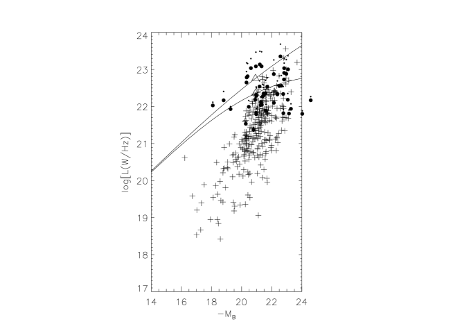
Figure 2: Optical Luminosity versus Radio Luminosity for the Condon sample (crosses) and for the B93 sample (filled circles) and for the B93 sample corrected to $z=0$ luminosity according to $L=L(z=0)(1+z)^{3.1}$ (filled squares). Over-plotted is the locus of the radio and optical flux limits for different redshifts, no evolution upper, de-evolved to $z=0$, lower

The $z\leq 0.35$ star-bursts from B93 are also plotted in Figure 2, as is the passage of its double flux limits to $z=0.35$.

The immediate point to notice from this Figure is that the $L,L_{B}$ plane is not well sampled by the B93 sample, the low radio luminosity region is poorly sampled. However this is due to the small volume at low redshift, there appears to be reasonable sampling across $L_{B}$ for a give radio luminosity.

For a non-evolving population, virtually all the radio sources lie above our optical limit at $z\leq 0.35$. In other words, if we regard our sample as a purely radio flux limited sample, then we can be confident of very high completeness to the radio flux limit. Rowan-Robinson et al. demonstrated that luminosity evolution of the same strength as required for IRAS galaxies $L(z)=L(z=0)(1+z)^{3.1}$ was sufficient to explain the sub-mJy radio counts. Such a pure luminosity evolution is equivalent to a large negative radio $K$-correction term, and the corrected positions in Figure 2 also demonstrate a high completeness.

We can quantify this by using the radio-optical correlation to estimate the incompleteness as a function of redshift, then use the observed redshift distribution to get a first-order estimate of the overall incompleteness:

$$f=100\%\times N_{\rm obs}/\sum k(L_{{\rm min},i},z_{i})=98.4\%$$ (6)

where $f$ is the completeness, $N_{\rm obs}$ the size of the star-burst sample, $k$ is $1$ over the fraction of the radio-optical correlation above the optical flux limit as a function of redshift and luminosity, $L_{{\rm min},i}$ is the faintest radio luminosity observable at redshift $z_{i}$, and the sum is performed over the star-burst sample. The B93 sample does appear to have a slightly larger dispersion in the radio-optical plane than the local sample, but this larger scatter still yields $96.7\%$ completeness. We conservatively assume no passive stellar evolution, the effect of which would be to increase our completeness further still. N.B. this measure of “completeness” is not the same as that described in Equation 4. The assertion that the optical selection does not have a significant additional impact on the radio selection is consistant with the findings from deep optical observations of the Marano Field (Gruppioni et al. in preparation) that the faintest optical identifications of sub-mJy radio sources do not appear to be star-burst galaxies.

3.3 $1/V$ Luminosity Function

The luminosity function is plotted in Figure 3, which agrees with the calculation in Rowan-Robinson et al. (1993). It is clear from Figure 3 that the faint end of the luminosity function is not well-constrained by this sample. This is due to the small volume at low redshift of this sample. For $z<0.05$ (where the limiting radio luminosity is $L=1.1\times 10^{21}h_{50}^{-2}{\rm WHz}^{-1}$ the B93 sample covers only $2700h_{50}^{-3}Mpc^{3}$, and using the S90 “warm” luminosity function we would only expect 1.75 galaxies within this volume. This small volume at low redshifts is also very susceptible to large scale structure variations. Assuming the power spectrum of Peacock and Dodds (1994) we would expect RMS density fluctuations of around 60 to 60 per cent over such a volume (allowing for the survey being spilt into three).

Figure 3: The $1/V$ Luminosity function for the B93 sample: filled circles. Also illustrated is the luminosity function from Condon 1987, upper curve, the warm IRAS luminosity function of S90, lower curve. Also illustrated is the estimate of luminosity function from Windhorst (1985)

The co-moving number densities are consistent with the single star-burst at $z<0.35$ detected in the Hubble Deep Field (Richards et al. 1998), as well as with the luminosity function from the $z<0.35$ Marano star-bursts (Gruppioni et al 1998, in preparation). This data is however in strong disagreement with the very high star-burst density claimed in the micro-Jansky radio population by Windhorst et al. (1995). Figure 3 plots the $z<0.35$ Windhorst et al. star-bursts, which have an order of magnitude higher space density than our estimate. The nature of the $\mu$Jy population is controversial however, with Hammer et al. (1995) claiming the population is dominated by weak AGN, albeit in a sky area which may be biased by the presence of a cluster. Part of the discrepancy may also be due to high frequency ($5-8.5$ GHz) selection in both the Hammer and Windhorst samples, where the radio spectral index may not be steep due to the flat-spectrum contributions from Hii regions and possibly AGN. The high-frequency selected sub-mJy/$\mu$Jy population may therefore be being sampled higher up the luminosity function, or may be contaminated by Seyfert galaxies. This justifies our choice of a low-frequency selected sub-mJy radio sample, albeit in retrospect.

3.4 Testing the shape of the luminosity function

We have already discussed that the B93 sample is insufficient to determine $\varphi(L)$ at faint radio luminosities since the volume and thus number of objects at low redshift is small.

To estimate the corrections to our estimate of the luminosity density (Equation 3) we are only interested in the shape of the luminosity function (where shape includes a measure of the typical Luminosity e.g. $L_{*}$) and not the overall normalisation which cancels in Equations 4 and 5. We thus wish to test the shape of B93 luminosity function against some reasonable a priori functions.

The IRAS luminosity function is well determined even at the faint end, it is natural to test an IRAS luminosity function modified via the FIR/radio correlation (Helou, Soifer & Rowan–Robinson 1985). For a galaxy with the model star-burst spectrum of Efstathiou, Rowan–Robinson & Seibenmorgen (1998, in preparation) this relation can be translated to

$$S_{60~{}\mu m}~{}=~{}133~{}S_{1.4~{}GHz}\\$$ (7)

or

$$L_{60~{}\mu m}~{}=~{}133~{}L_{1.4~{}GHz}\\$$ (8)

We consider two models, the first ($l1$) is the “warm” luminosity function of S90(their solution 25), (modified so $L_{*}=133L_{60*}$). It is appropriate to use the “warm” sample, since these are the actively star-forming galaxies, similar to this sample. This luminosity function is also clearly similar in shape and normalisation to our observed radio luminosity function (Figure 3). The use of this model luminosity function is independent of the overall normalisation, and assumes the shape is constant with redshift. It is known that IRAS galaxies strongly evolve (e.g. S90, Oliver et al 1994, etc.), and if this evolution only changes the normalisation of the luminosity function then this is immaterial. However if shape of the luminosity function was to change with redshift, this would affect our estimate of the luminosity density. Neither IRAS samples, nor this sample alone are sufficient to determine what sort of evolution is appropriate to these types of samples; however the faint radio counts do not support pure density evolution as strong as that suggested in S90 (Rowan-Robinson et al. 1993). Thus it is appropriate to consider some model with an evolution of the Luminosity with redshift. Our second model $l2$ assumes the same zero redshift luminosity function as $l1$ but has $L=L_{0}(1+z)^{3.1}$. Since the S90 $z=0$ luminosity function was not calculated with this evolution, this model is not entirely consistent and will over-predict the numbers of luminous galaxies, and lead to an under-correction to the Luminosity density, nevertheless the two models together give a reasonable idea of the level of uncertainty in the luminosity function, and would bracket a more natural model where Luminosity evolution was included in the estimate of the Luminosity function self consistently.

Our third model, $l3$, assumes the shape of the low $z$ Condon et al (1987) radio luminosity function, with no evolution.

In addition to the luminosity functions we consider a number of different models for the effect of the joint optical and radio limits on the observable radio luminosities $P_{i}({\cal O}|L)$:

$$P_{i}({\cal O}|L)=\frac{\Omega(S(L,z_{i}))}{\Omega_{\rm max}}$$ (9)

$$P_{i}({\cal O}|L)=\frac{\Omega(S(L,z_{i}))}{\Omega_{\rm max}}\frac{\Omega_{B}(S_{B}(LL_{B,i}/L_{i},z_{i}))}{\Omega_{B,\rm max}}$$ (10)

$$P_{i}({\cal O}|L)=\frac{\Omega(S(L,z_{i}))}{\Omega_{\rm max}}\frac{\int_{\infty}^{+\infty}\Omega_{B}P(L_{B}|L)dlgL_{B}}{\Omega_{B,\rm max}}$$ (11)

(In the above equations $B$ represents the optical which may be either $B$ or $V$ band, where corresponding magnitudes of individual objects are computed using the $S_{5000}/S_{7000}$ ratio in B93 and magnitude limits are adjusted using the average $m_{B}-m_{V}=0.7$.) Model $m0$ (Equation 9) assumes that the optical magnitude of the object is totally unrelated to the radio luminosity so the only selection that comes into play is the radio flux limit. If we knew the radio flux limit as a function of position Equation 9 would reduce to $P_{i}({\cal O}|L)=0,L<L_{{\rm min},i};P_{i}({\cal O}|L)=1,L\geq L_{{\rm min},i}$. Equation 10 (model $m1$), assumes that the lower luminosity objects potentially missed through the optical selection have the same radio/optical colour as the object under consideration, this will be satisfactory if the colours within the sample are representative of the colours in the underlying population (in fact the optical and radio flux limits will survey to restrict the range of colours); in our case of simple magnitude limits $\Omega_{B}/\Omega_{B,\rm max}=0,S_{B}<S_{B,\rm lim};s\Omega_{B}/\Omega_{B,\rm max}=1,S_{B}\geq S_{B,\rm lim}$. Model $m2$ (and $m3$) take the form of Equation 11 and require some estimate for the marginal optical radio distribution function $P(L_{B}|L)$: model $m2$ takes this from Saunders et al. (1990, S90), assuming $L_{60}=133L$; model $m3$ takes this from the Condon et al (1991).

Using the different models ($m0,m1,m2,m3$) for the optical and radio selection criteria $P_{i}({\cal O}|L)$ and the three models for the luminosity function $l1,l2,l3$ we calculate the luminosity distributions and compare with the observed luminosity distributions using a K-S test, these results are summarised in Table 1. (In this and subsequent analysis we have excluded the 5 objects which fall below the optical completeness limits quoted in Benn et al..) From this we can see that none of the models tested can be significantly ruled out. There is very little difference between the models which assume either no optical selection effects or optical selection effects determined from a priori estimates of the radio/optical distribution, this is because these estimates do not predict any significant loss of sources to the optical selection effects. A better fit is provide by models which assume the optical selection is determined by the distribution of colours within the sample itself ($m1$). All forms of luminosity function give acceptable fits, assuming $m1$.

$P_{i}({\cal O}|L)$	$m0$	$m1$	$m2$	$m3$
$\varphi(L)$	$l1$	$l1$	$l1$	$l1$
$P(KS)$	0.13	0.64	0.13	0.13
$P_{i}({\cal O}|L)$	$m0$	$m1$	$m2$	$m3$
$\varphi(L)$	$l2$	$l2$	$l2$	$l2$
$P(KS)$	0.30	0.83	0.29	0.30
$P_{i}({\cal O}|L)$	$m0$	$m1$	$m2$	$m3$
$\varphi(L)$	$l3$	$l3$	$l3$	$l3$
$P(KS)$	0.04	0.33	0.04	0.04

Table 1: Comparison of the observed and expected luminosity distributions under various assumptions about the underlying luminosity function and selection effects.

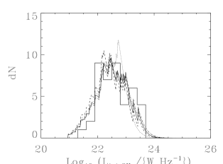
Figure 4: The observed and expected luminosity distributions. Solid histogram, observed distribution. Dotted curve expected luminosity distribution assuming “warm” IRAS luminosity function ($l1$) and no accounting for optical selection ($m0$, similar to $m2,m3$). Solid curve $l1$ and optical selection determined by objects colours ($m1$). Dot-dashed curve, evolving “warm” IRAS luminosity function ($l2$). Dashed curve Condon Luminosity function ($l3$).

3.5 The luminosity density

The correction factor ($C({L_{\rm min},L_{B,{\rm min}}})$, Equation 4) to be applied to the luminosity density in the presence of luminosity (i.e. redshift) cuts, can be re-expressed and estimated in a number of ways, we choose to express it as

$$C = \frac{\int_{L_{\rm min}}^{+\infty}L\varphi(L)d\log L}{\int_{-\infty}^{+\infty}L\varphi(L)d\log L}$$ (12)

$$- \frac{\int_{L_{\rm min}}^{+\infty}\int_{L_{B,{\rm min}}}^{+\infty}L\varphi(L,L_{B})d\log L_{B}d\log L}{\int_{-\infty}^{+\infty}\int_{-\infty}^{+\infty}L\varphi(L,L_{B})d\log L_{B}d\log L}.$$

The last term in this equation represents the loss in luminosity density due to the optical cuts alone. We have calculated this term at $z=0.05$ and $z=0.175$ using the Condon bivariate luminosity function, the Saunders bivariate luminosity function, and for a version of the Condon bivariate luminosity function with increased dispersion appropriate for the B93 sample. The largest value we get for the second term is ${\cal O}10^{-5}$, which is negligible compared to the former term involving only the radio luminosity density ${\cal O}1$. Since the normalisation cancels out, the only significant correction to be applied is due to the shape of the luminosity function.

With surveys of small volume density fluctuations on the scale of the survey volume can contribute significantly to the uncertainty in derived quantities. To estimate the errors due to this cosmic variance we determine the effective wavenumber $k$ appropriate for a cube with volume one third of the total volume in the redshift range, since the survey is composed of three independent volumes. From this we can estimate the density fluctuations $\sigma^{2}=\Delta^{2}(k)$ from the power spectrum of Peacock and Dodds (1994), these we reduce by a factor of three, assuming the three separate areas are independent. These errors are approximate and do not take properly into account the survey geometry or the fact that lower luminosity objects sample smaller volumes, all these effects would serve to increase the errors. These errors are slightly larger than the shot noise terms to which they are added in quadrature. We tabulate the cosmic variance errors for this and other samples used for estimating luminosity densities(Table 2).

Sample	Area	sub.	$z_{\rm min}$, $z_{\rm max}$	$k_{\rm eff}/h_{50}$	$\sigma$
	$/10^{-4}$sr			/${\rm Mpc}^{-1}$
B93:	3.4	3	0, 0.05	0.30	0.72
B93:	3.4	3	0.05, 0.175	0.095	0.41
B93:	3.4	3	0.175, 0.35	0.055	0.26
B93:	3.4	3	0.05, 0.35	0.052	0.25
B93:	3.4	3	0, 0.35	0.052	0.25
Tresse &	0.42	5	0, 0.3	0.040	0.16
Maddox:
Lilly	0.42	5	0.2, 0.5	0.028	0.10
Lilly	0.42	5	0.5, 0.75	0.024	0.088
Lilly	0.42	5	0.75, 1	0.023	0.079
Gallego	1400	1	0, 0.045	0.0089	0.036
Gronwall	210	1	0, 0.085	0.0092	0.017

Table 2: Cosmic variance errors ($\sigma=\sqrt{\Delta^{2}(k)}$) within surveys of different areas, redshift ranges and different number of subdivisions. For the B93, Tresse & Maddox and the low $z$ Lilly samples these errors are comparable with the shot noise errors.

In Table 3 we tabulate the un-corrected luminosity density for the B93 sample over 4 redshift ranges. We also tabulate the correction factors that need to be applied assuming various luminosity functions which we have shown to be compatible with this sample, (for the evolving luminosity function we have take then luminosity function shape to be defined at roughly the centre of the redshift bin). We also tabulate the luminosity density estimated from a Schecter function fit to the luminosity function Condon RSA excluding AGN (Serjeant et al, in preparation). We also tabulate the luminosity density for warm IRAS galaxies from S90, scaled by $\Phi_{60\mu{\rm m}}=133\Phi_{1.4}$.

$z$	$\log\Phi_{1.4}$	$-\log C(L_{\rm min},B_{\rm min})$
	$/h_{50}{\rm WHz}^{-1}{\rm Mpc}^{-3}$	$l1$	$l2$	$l3$
0-0.05	$19.27\pm 0.14$	0.0	0.0	0.0
0-0.35	$19.09\pm 0.14$	0.0	0.0	0.0
0.05-0.35	$19.09\pm 0.14$	0.03	0.02	0.05
0.05-0.175	$18.91\pm 0.20$	0.03	0.02	0.05
0.175-0.35	$19.01\pm 0.16$	0.21	0.12	0.42
0-0.1	$18.69\pm 0.05$	0.0	0.0	0.0
0-0.1	$19.08\pm 0.04$	0.0	0.0	0.0

Table 3: Estimates of the raw 1.4GHz luminosity density in different redshifts ranges and corrections that need to be applied under different assumptions about the underlying luminosity function. The $0<z<0.05$ luminosity density is taken from Serjeant et al. (in preparation). The last two rows are obtained from converting the “warm” and total IRAS luminosity densities of S90 to a 1.4Ghz luminosity density using $133L_{1.4}=L_{60}$.

We can see from this that the total luminosity density in the B93 sample as a whole is in good agreement with the luminosity density from the Condon sample. The luminosity density in the higher redshift bin is larger than that in the lower redshift bin by a factor of between 1.7 and 3.7, depending on the luminosity function applied, consistent with luminosity evolution at a rate of $(1+z)^{3.1}$, however, due to the cosmic variance this is not very significant.

The luminosity density from the low-redshift sample alone is a factor of around two lower than the Condon sample and similar to the luminosity density as estimated from the “warm” IRAS galaxies. Due to the cosmic variance the discrepancy with the Condon sample is not significant, while the discrepancy between the Condon sample and the “warm” IRAS sample is. It is likely that the Condon sample also includes the radio equivalent of the IRAS “cool” Cirrus galaxies.

Using the $H\alpha$ luminosities quoted in Benn et al 1993, corrected for slit loss using the APM magnitudes and continuum fluxes we can use the same effective volumes to estimate the $H\alpha$ luminosity density within this sample, Table 4. This may be an underestimate of the total $H\alpha$ luminosity density since from some objects $H\alpha$ is not detected and we have not included the spectroscopic limits in our effective volume.

$z$	$\Phi(H\alpha)$
	$/h_{50}{\rm W}Mpc^{-3}$
0.0-0.35	31.8627
0.05-0.35	31.7764
0.05-0.175	31.7554
0.175-0.35	31.2052

Table 4: $H\alpha$ Luminosity density estimated from star-forming galaxies within the B93 sample. Errors and correction factors will be similar to those in 3

4 Conversion from Luminosity Density to star formation rate

Nearly all of the radio emission from star–forming galaxies is synchrotron radiation from relativistic electrons and free-free emission from Hii regions. Only massive stars (i.e. $M~{}{{}_{>}\atop{}^{\sim}}~{}5M_{\odot}$) ionise the Hii regions and produce supernovae, whose remnants accelerate most of the relativistic electrons. Such massive stars have lifetimes much shorter than the Hubble time, so the current radio luminosity is proportional to the recent star formation rate (Condon 1992). The supernova rate is directly related to the non–thermal radio luminosity, which at $1.4$ GHz is dominant over the thermal component (see Condon & Yin 1990 for the most reliable derivation of this relation, calibrated with Galactic supernova remnants). Moreover, since all stars more massive than $M=5M_{\odot}$ become radio supernovae, the radio supernova rate is determined directly by the star formation rate. Thus, the star formation rate can be obtained by non–thermal radio luminosity, following Condon (1992):

$$SFR(M\geq 5M_{\odot})=\frac{L_{1.4~{}GHz}~{}[WHz^{-1}]}{5.3\times 10^{21}(\frac{\nu}{GHz})^{\alpha}}~{}M_{\odot}yr^{-1}$$ (13)

where $\nu$ is the frequency and $\alpha$ is the non–thermal radio spectral index (as defined above). If we assume a Salpeter initial mass function (IMF; $\psi(M)\propto M^{-2.35}$, $0.1-125$ $M_{\odot}$) we obtain for the total star formation rate

$$SFR(M\geq 0.1M_{\odot})=\frac{L_{1.4~{}GHz}~{}[WHz^{-1}]}{7.63\times 10^{20}}$$ (14)

In Figures 5, 6 we convert our radio luminosity densities (Table 3, row 3, correction $l1$) to star formation rates together with that from the RSA sample (Table 3, row 1).

It is instructive to compare with the U-band luminosity densities at redshifts $z\stackrel{{\scriptstyle<}}{{{}_{\sim}}}1$, from Treyer et al. (1998) and the Canada-France Redshift Survey (CFRS, Lilly et al. 1996). For the ultraviolet conversions we assume

$$SFR(M\geq 0.1M_{\odot})=\frac{L_{2000\AA}~{}[W]}{7.94\times 10^{20}}$$ (15)

$$SFR(M\geq 0.1M_{\odot})=\frac{L_{2500\AA}~{}[W]}{6.7\times 10^{20}}$$ (16)

taken from Treyer et al. (1998) and Cowie et al. (1997) respectively. In Figure 5 we do not apply a reddening correction, in Figure 6 the luminosity densities are de-reddened following Treyer et al. (1998).

Also plotted are the H$\alpha$ luminosity densities from the CFRS (Tresse & Maddox 1997) the KISS sample (Gromwell 1998) and from the local ($z=0$) sample of Gallego et al. (1995), converted to total star formation rates for this IMF using

$$SFR(M\geq 0.1M_{\odot})=\frac{L_{H\alpha}~{}[W]}{1.41\times 10^{34}}$$ (17)

from Madau et al. (1996). Both H$\alpha$ luminosity densities were corrected for reddening using Balmer decrements and assuming a simple dust screen, in Figure 5 we remove the average reddening correction $\sim 1$ mag (Tresse & Maddox 1997).

Figure 5: The co-moving star-formation rate $z<1$ as estimated from: Filled circles = 1.4GHz (Left to right: Condon, B93) Open circles = $H\alpha$ (Gallego, Gromwell, B93, Tresse & Maddox) Open triangles = UV (Treyer, Lilly, Lilly, Lilly). Corrections for reddening have not been made or have been removed

Figure 6: The co-moving star-formation rate $z<1$ as estimated from: Filled circles = 1.4GHz (Left to right: Condon, B93) Open circles = $H\alpha$ (Gallego, Gromwell, B93, Tresse & Maddox) Open triangles = UV (Treyer, Lilly, Lilly, Lilly) Corrections for reddening have been made or retained

A priori we would have expected the 1.4GHz to provide a higher estimate of the star-formation rate than an un-reddened optical estimate. This is because the radio should be measuring the total star-formation rate which the optical only measures the un-obscured rate. At the low redshift ($0<z<0.05$) this does indeed appear to be the case, the Condon luminosity density is well above that estimated from the $H\alpha$ of Gallego et al. (1995) and Gromwell (1998), and above the UV estimate of Treyer et al. (1998). At intermediate redshifts ($0.05<z<0.35$), probed by the B93 survey, the Tress & Maddox $H\alpha$ estimate from the CFRS and the UV estimate of Treyer et al. (1998), the estimates agree, if the reddening corrections are applied then the optical estimators can even exceed the radio estimate (Figure 6). This is initially surprising until we notice that the errors are large, we note that we have applied the cosmic variance terms to all the data points and these are significant, particularly for the B93 sample and the Tresse & Maddox sample. We thus suspect that the coincidence of these various estimators may be due to differences in the mean density of these survey volumes which masks a difference in their sampling of the star-formation rate. This assertion is strengthened when we see that the $H\alpha$ estimate of the star-formation rate from the B93 sample itself is further below the radio estimate than the Tresse & Maddox point is above it.

An additional star-formation indicator is the far infrared. Several authors (Scoville & Young 1983; Thronson & Telesco 1986; Condon 1992; Rowan–Robinson et al. 1997) have derived relations to convert from 60 $\mu$m luminosity to star formation rate. These calculations assume some proportion of the optical luminosity produced by young stars is absorbed and re-emitted in the infrared. (This same extinction factor should naturally be applied to the star-formation rates calculated from the UV.) From such calculations it is of course possible to deduce the FIR/Radio correlation. Condon (1992) deduced the FIR/Radio correlation assuming an obscuration factor of 2/3., recently Cram et al. (1998) seems to indicate a close agreement between the radio SFR estimate and the far–infrared one obtained considering $\sim 100$ per cent reprocessing of starlight in the far-infrared. In general it does appear that the extinction fraction is high. It would in fact be possible to use the FIR/Radio correlation to determine the extinction fraction for any assumed underlying IMF, this could then be feed self consistently into the UV and $H\alpha$ SFR estimates. Such an analysis is beyond the scope of this paper.

Instead we use the FIR/Radio correlation simply to convert local estimates of the $60\mu$m luminosity density from S90 to 1.4GHz luminosity density and then use the 1.4GHz calibration above which is independent of extinction. We plot in Figure 5,6 the star-formation rate estimated thus from the S90 luminosity densities for both “warm” IRAS galaxies and for all IRAS galaxies. It is not clear that the “cool” IRAS galaxies trace star-formation as do the warm IRAS galaxies, since the cool emission is from cirrus clouds which may be illuminated by older stellar populations (similarly the UV density of quiescent or weakly star-forming galaxies might also be dominated by old stars).

5 Conclusion

We have estimated the 1.4 GHz luminosity density from a sample of radio star-burst galaxies $z<0.35$, demonstrating that the optical selection criteria applied to this sample are not important to this determination. The small volume of this survey at $z<0.05$ prevents us from having accurate estimates of the luminosity density from low radio luminosity star-forming galaxies. Nevertheless we demonstrate that a number of reasonable a priori luminosity functions can be used to estimate the luminosity density missed. These corrections are small for the sample as a whole, though larger and more disparate for a higher redshift sub-sample. The 1.4 GHz luminosity density increases as we move to higher redshifts, though the strength of this effect is dependent on the assumed luminosity function and may not be conclusive with a sample of this volume. Overall the 1.4 GHz luminosity density agrees with that obtained from 1.4 GHz measurements of the RSA sample of Condon et al..

The 1.4GHz estimator of star-formation rates should be unaffected by extinction, whereas local estimates from the UV and $H\alpha$ should be. We were thus surprised to find the estimate from the radio broadly consistent with these other estimates, particularly since the local estimate from the Condon luminosity density was considerably higher than from optical measures. Since the luminosity density estimated from $H\alpha$ within the B93 sample produces a much lower estimate of the star-formation rate than the 1.4GHz estimate and the (optimistic) cosmic variance errors in the B93 and CFRS samples are comparable to the shot noise errors we attribute this apparent agreement to clustering fluctuations. We thus strongly suggest that spectroscopic follow-up of larger area radio surveys is needed to accurately determine the un-obscured star-formation rates $0<z<0.3$.

The star formation rates at these redshifts do not conflict with the Far-IR background measurements, since the sub-mJy radio population make a negligible contribution to the FIR background. At these redshifts the $1.4$ GHz and $850\mu$m fluxes are roughly equal, and the Puget et al. (1996) $850\mu$m background corresponds to about $26$ Jy per square degree.

References

- [1] Baugh C.M., Cole S., Frenk C.S. & Lacey C.G., 1998, ApJ, 498, 504
- [2] Benn C.R., Rowan–Robinson M., McMahon R.G., Broadhurst T.J. & Lawrence A., 1993, MNRAS, 263, 98
- [3] Condon J.J., 1987, ApJS, 65, 485
- [4] Condon J.J., 1992, ARA&A, 30, 575
- [5] Condon J.J. & Mitchell K.J., 1984, AJ, 89, 610
- [6] Condon J.J & Yin Q.F., 1990, ApJ, 357, 97
- [7] Cram L., Hopkins A., Mobasher B. & Rowan–Robinson M., 1998, MNRAS, in press (astro–ph/9805327)
- [8] Gallego, J., Zamorano, J., Aragon-Salamanca, A., Rego, M., 1995, ApJ, 455, L1
- [9] Hammer F., Crampton D., Lilly S.J., Le Fèvre O. & Kenet T., 1995, MNRAS, 276, 1085
- [10] Helou G., Soifer B.T. & Rowan–Robinson M., 1985, ApJL, 298, L7
- [11] Lilly s.J., Le Fevre O., Hammer F. & Crampton D., 1996, ApJL, 460, L1
- [12] Kennicutt R.C., 1983, ApJ, 272, 54
- [13] Kron R.G., Koo D.C. & Windhorst R.A., 1985, A&A, 146, 38
- [14] Madau P., Ferguson H.C., Dickinson M.E., Giavalisco M., steidel C.C., Fruchter A., 1996, MNRAS, 283, 1388
- [15] Metcalfe N., Shanks T., Fong R., Jones L.R. 1991, MNRAS, 249, 498
- [16] Mitchell K.J. & Condon J.J., 1985, AJ, 90, 1957
- [17] Oliver S. et al. 1995 in Proc. 35th Herstmonceux Conf. ‘Wide-Field Spectroscopy and the Distant Universe’ eds. S.J. Maddox and A. Aragon-Salamanca. (World Scientific) p. 274
- [18] Oort M.J.A., 1987a, PhD Thesis, Univ. of Leiden
- [19] Oort M.J.A., 1987b, A&AS, 71, 221
- [20] Peacock J. A., Dodds S.J., 1994 MNRAS 267, 1020
- [21] Pei Y.C. & Fall S.M., 1995, ApJ, 454, 69
- [22] Pettini M., King D.L., Smith L. & Hunstead R.W., 1997, ApJ, 478, 536
- [23] Puget J.-L., Abergel A., Bernard J.-P., Boulanger F., Burton W.B., Desert F.-X. & Hartmann D., 1996, A&A, 308, 5
- [24] Richards R.E., Kellermann K.I., Fomalont E.B., Windhorst R.A. & Partridge R.B., 1998, ApJ, in press (astro–ph/9803343)
- [25] Rowan–Robinson M., Benn C.R., Lawrence A., McMahon R.G & Broadhurst T.J., 1993, MNRAS, 263, 123
- [26] Rowan–Robinson M. et al., 1997, MNRAS, 289, 490
- [27] Saunders W., Rowan–Robinson M., Lawrence A., Efstathiou G., Kaiser N., Frenk C.S., 1990 (S90), MNRAS, 242, 318
- [28] Schmidt M., 1968, ApJ, 151, 393
- [29] Scoville N.Z. & Young J.S., 1983, ApJ, 265, 148
- [30] Thronson H. & Telesco C., 1986, ApJ, 311, 98
- [31] Thuan T.X. & Condon J.J., 1987, ApJL, 322, L9
- [32] Windhorst R.A., 1984, PhD Thesis, Univ. of Leiden
- [33] Windhorst R.A., Miley G.K., Owen F.N., Kron R.G. & Koo D.C., 1985, ApJ, 289, 494
- [34] Windhorst R.A., Fomalont E.B., Kellermann K.I., Partridge R.B., Richards E., Franklin B.E., Pascarelle S.M. & Griffiths R.E., 1995, Nature, 375, 471