Positron Propagation and Fluxes from Neutralino Annihilation in the Halo

Abstract

Supersymmetric neutralinos are one of the most promising candidates for the dark matter in the Universe. If they exist, they should make up some fraction of the Milky Way halo. We investigate the fluxes of positrons expected at the Earth from neutralino annihilation in the halo. Positron propagation is treated in a diffusion model including energy loss. The positron source function includes contributions from both continuum and monochromatic positrons. We find that, for a “canonical” halo model and propagation parameters, the fluxes are generally too low to be visible. Given the large uncertainties in both propagation and halo structure, it is however possible to obtain observable fluxes. We also investigate the shapes of the positron spectra, including fits to a feature indicated by the results of the Heat experiment.

I Introduction

It is well known that a large fraction of the mass of the Universe has only been observed by its gravitational effects. The nature of this dark matter is unknown. Standard Big Bang Nucleosynthesis bounds the baryon density of the Universe, but these results fall far short of the known amount of dark matter. Thus more exotic forms of matter are sought, and weakly interacting massive particles (WIMPs) are one of the most promising cold dark matter candidates.

Perhaps the best WIMP candidate is the neutralino (for a review, see Ref. [1]), which arises in supersymmetric models as a linear combination of the superpartners of the neutral gauge and Higgs bosons. We choose the neutralino as our WIMP candidate, though we allow its properties to vary over a generous sample of supersymmetric models.

It may be possible to detect neutralinos (or WIMPs) in the galactic halo by the products of their mutual annihilations, e.g. by searching for gamma rays [2], antiprotons [3] and positrons [4, 5, 6] coming from the Milky Way halo. In this paper we consider neutralino annihilation in the halo into positrons (both continuum and monochromatic). Compared to earlier studies [4, 5, 6], we will use a true diffusion model instead of a leaky-box model. This has the advantage of allowing us to use more realistic models for the diffusion constant while still permitting an analytic solution. The numerical implementation is very fast, making detailed scans over the huge MSSM parameter space feasible. We also include all two-body final states of neutralino annihilation (at tree level) using detailed Monte Carlo simulations for the decay and/or hadronization of the annihilation products. We will compare our results mainly with those of Kamionkowski and Turner [6] (hereafter KT).

We will also compare our predictions of the positron fluxes to observations. The fluxes are typically small compared to the expected background, but given the large uncertainties involved, we identify models that can have a significant effect on the observed positron spectrum. We will show that a large class of models improves the fit of observations to the predicted background. Finally, we investigate the positron spectra at higher energies than have been observed, and identify features that may be detectable by future experiments such as Ams [7].

II Set of supersymmetric models

We work in the Minimal Supersymmetric Standard Model (MSSM). In general, the MSSM has many free parameters, but with some reasonable assumptions we can reduce the number of parameters to the Higgsino mass parameter $\mu$, the gaugino mass parameter $M_{2}$, the ratio of the Higgs vacuum expectation values $\tan\beta$, the mass of the $CP$-odd Higgs boson $m_{A}$, the scalar mass parameter $m_{0}$ and the trilinear soft SUSY-breaking parameters $A_{b}$ and $A_{t}$ for the third generation. In particular, we don’t impose any restrictions from supergravity other than gaugino mass unification. We have made some scans without the GUT relation for the gaugino mass parameters $M_{1}$ and $M_{2}$. This mainly has the effect of allowing lower neutralino masses to escape the LEP bounds and is not very important for this study. Hence, the GUT relation for $M_{1}$ and $M_{2}$ is kept throughout this paper. For a more detailed definition of the parameters and a full set of Feynman rules, see Refs. [8, 9].

The lightest stable supersymmetric particle is in most models the lightest neutralino, which is a superposition of the superpartners of the gauge and Higgs fields,

$$\tilde{\chi}^{0}_{1}=N_{11}\tilde{B}+N_{12}\tilde{W}^{3}+N_{13}\tilde{H}^{0}_{1}+N_{14}\tilde{H}^{0}_{2}.$$ (1)

It is convenient to define the gaugino fraction of the lightest neutralino,

$$Z_{g}=|N_{11}|^{2}+|N_{12}|^{2}.$$ (2)

For the masses of the neutralinos and charginos we use the one-loop corrections as given in Ref. [10] and for the Higgs boson masses we use the leading log two-loop radiative corrections, calculated within the effective potential approach given in Ref. [11].

We make extensive scans of the model parameter space, some general and some specialized to interesting regions. In total we make 18 different scans of the parameter space. The scans are done randomly and are mostly distributed logarithmically in the mass parameters and in $\tan\beta$. For some scans the logarithmic scan in $\mu$ and $M_{2}$ has been replaced by a logarithmic scan in the more physical parameters $m_{\chi}$ and $Z_{g}/(1-Z_{g})$ where $m_{\chi}$ is the neutralino mass. Combining all the scans, the overall limits of the seven MSSM parameters we use are given in Table I.

We check each model to see if it is excluded by the most recent accelerator constraints, of which the most important ones are the LEP bounds [12] on the lightest chargino mass,

$$m_{\chi_{1}^{+}}>\left\{\begin{array}[]{lcl}91{\rm~{}GeV}&\quad,&|m_{\chi_{1}^{+}}-m_{\chi^{0}_{1}}|>4{\rm~{}GeV}\\ 85{\rm~{}GeV}&\quad,&{\rm otherwise}\end{array}\right.$$ (3)

and on the lightest Higgs boson mass $m_{H_{2}^{0}}$ (which range from 72.2–88.0 GeV depending on $\sin(\beta-\alpha)$ with $\alpha$ being the Higgs mixing angle) and the constrains from $b\to s\gamma$ [13]. For each allowed model we calculate the relic density of neutralinos $\Omega_{\chi}h^{2}$, where $\Omega_{\chi}$ is the density in units of the critical density and $h$ is the present Hubble constant in units of $100$ km s^-1 Mpc^-1. We use the formalism of Ref. [14] for resonant annihilations, threshold effects, and finite widths of unstable particles and we include all two-body tree-level annihilation channels of neutralinos. We also include the so-called coannihilation processes in the relic density calculation according to the analysis of Edsjö and Gondolo [8].

Present observations favor $h=0.6\pm 0.1$, and a total matter density $\Omega_{M}=0.3\pm 0.1$, of which baryons may contribute 0.02 to 0.08 [15]. Not to be overly restrictive, we accept $\Omega_{\chi}h^{2}$ in the range from $0.025$ to $1$ as cosmologically interesting. The lower bound is somewhat arbitrary as there may be several different components of non-baryonic dark matter, but we demand that neutralinos are at least as abundant as required to make up the dark halos of galaxies. In principle, neutralinos with $\Omega_{\chi}h^{2}<0.025$ would still be relic particles, but only making up a small fraction of the dark matter of the Universe. We will only consider models with $\Omega_{\chi}h^{2}<0.025$ when discussing the dependence of the signal on $\Omega_{\chi}h^{2}$.

Parameter	$\mu$	$M_{2}$	$\tan\beta$	$m_{A}$	$m_{0}$	$A_{b}/m_{0}$	$A_{t}/m_{0}$
Unit	GeV	GeV	1	GeV	GeV	1	1
Min	-50000	-50000	1.0	0	100	-3	-3
Max	50000	50000	60.0	10000	30000	3	3

TABLE I.: The ranges of parameter values used in our scans of the MSSM parameter space. Note that several special scans aimed at interesting regions of the parameter space has been performed. In total we have generated approximately 103000 models that are not excluded by accelerator searches.

III Positron spectra from neutralino annihilation

When neutralinos annihilate in the galactic halo they produce quarks, leptons, gauge bosons, Higgs bosons and gluons. When these particles decay and/or hadronize, they will give rise to positrons either directly or from decaying mesons in hadron jets. We thus expect to get both monochromatic positrons (at an energy of $m_{\chi}$) from direct annihilation into $e^{+}e^{-}$ and continuum positrons from the other annihilation channels. In general the branching ratio for annihilation directly into $e^{+}e^{-}$ is rather small, but for some classes of models one can obtain a large enough branching ratio for the line to be observable.

For continuum positrons, we simulate the decay and/or hadronization with the Lund Monte Carlo Pythia 6.115 [16]. We perform the simulation for a set of 18 different neutralino masses from 10 to 5000 GeV and for the “basic” annihilation channels consisting of the heavy quarks, leptons and gauge bosons. The annihilation channels containing Higgs bosons are then easily taken into account by allowing the Higgs bosons to decay in flight and averaging the produced positron flux over the decay angles. For any given MSSM model, the positron spectrum is then given by

$$\frac{d\phi}{d\varepsilon}=\left.\frac{d\phi}{d\varepsilon}\right|_{\rm cont.}+\left.\frac{d\phi}{d\varepsilon}\right|_{\rm line}=\sum_{F\neq e^{+}e^{-}}B_{F}\left.\frac{d\phi}{d\varepsilon}\right|_{F}+B_{e^{+}e^{-}}\,\delta(\varepsilon-\tilde{m}_{\chi}),$$ (4)

in units of $e^{+}/{\rm annihilation}$ where $\varepsilon=E_{e^{+}}/({\rm 1~{}GeV})$, $\tilde{m}_{\chi}=m_{\chi}/({\rm 1~{}GeV})$, $B_{F}$ is the branching ratio into a given final state $F$ and $\left.d\phi/d\varepsilon\right|_{F}$ is the spectrum of positrons from annihilation channel $F$. We include all two-body final states (except the three lightest quarks which are completely negligible) at tree level and the $Z\gamma$ [17] and $gg$ [18] final states which arise at one-loop level.

IV Propagation model

A Propagation and the interstellar flux

We consider a standard diffusion model for the propagation of positrons in the galaxy. Charged particles move under the influence of the galactic magnetic field. With the energies we are concerned with, the magnetic gyroradii of the particles are quite small. However, the magnetic field is tangled, and even with small gyroradii, particles can jump to nearby field lines which will drastically alter their courses. This entire process can be modeled as a random walk, which can be described by a diffusion equation.

Positron propagation is complicated by the fact that light particles lose energy quickly due to inverse Compton and synchrotron processes. Diffuse starlight and the Cosmic Microwave Background (CMB) both contribute appreciably to the energy loss rate of high energy electrons and positrons via inverse Compton scattering. Electrons and positrons also lose energy by synchrotron radiation as they spiral around the galactic magnetic field lines.

Our detailed treatment of positron diffusion follows. First we define a dimensionless energy variable $\varepsilon=E/(1\;{\rm GeV})$. The standard diffusion-loss equation for the space density of cosmic rays per unit energy, $dn/d\varepsilon$, is given by

$$\frac{\partial}{\partial t}\frac{dn}{d\varepsilon}=\vec{\nabla}\cdot\left[K(\varepsilon,\vec{x})\vec{\nabla}\frac{dn}{d\varepsilon}\right]+\frac{\partial}{\partial\varepsilon}\left[b(\varepsilon,\vec{x})\frac{dn}{d\varepsilon}\right]+Q(\varepsilon,\vec{x}),$$ (5)

where $K$ is the diffusion constant, $b$ is the energy loss rate and $Q$ is the source term. We will consider only steady state solutions, setting the left hand side of Eq. (5) to zero.

We assume that the diffusion constant $K$ is constant in space throughout a “diffusion zone”, but it may vary with energy. At energies above a few GeV, we can represent the diffusion constant as a power law in energy [19],

$$K(\varepsilon)=K_{0}\varepsilon^{\alpha}\approx 3\times 10^{27}\varepsilon^{0.6}{\rm cm}^{2}\;{\rm s}^{-1}.$$ (6)

However, at energies below about 3 GeV, there is a cutoff in the diffusion constant that can be modeled as

$$K(\varepsilon)=K_{0}\left[C+\varepsilon^{\alpha}\right]\approx 3\times 10^{27}\left[3^{0.6}+\varepsilon^{0.6}\right]{\rm cm}^{2}\;{\rm s}^{-1}.$$ (7)

We will in the following consider both of these models for the diffusion constant, but we will focus on the second expression. We will refer to Eq. (6) as model A and Eq. (7) as model B. The function $b(\varepsilon)$ represents the (time) rate of energy loss. We allow energy loss via synchrotron emission and inverse Compton scattering. The rms magnetic field in the diffusion zone is about $3~{}\mu$G, an energy density of about 0.2 eV cm^-3. We allow inverse Compton scattering on both the cosmic microwave background and diffuse starlight, which have energy densities of 0.3 and 0.6 eV cm^-3 respectively. These two processes combined give an energy loss rate [20]

$$b(\varepsilon)_{e^{\pm}}=\frac{1}{\tau_{E}}\varepsilon^{2}\approx 10^{-16}\varepsilon^{2}\;{\rm s}^{-1},$$ (8)

where we have neglected the space dependence of the energy loss rate. The function $Q$ is the source of positrons in units of cm^-3 s^-1.

The diffusion zone is a slab of thickness $2L$. We will fix $L$ to be 3 kpc, which fits observations of the cosmic ray flux [19]. We impose free escape boundary conditions, namely that the cosmic ray density drops to zero on the surfaces of the slab, which we let be the planes $z=\pm L$. We neglect the radial boundary usually considered in diffusion models. This is justified when the sources of cosmic rays are nearer than the boundary, as is usually the case with galactic sources. We will see that the positron flux at Earth, especially at higher energies, mostly originates within a few kpc and hence this approximation is well justified in our case.

We will now consider the diffusion-loss equation, Eq. (5), in the steady-state. We first make a change of variables, $u=1/\varepsilon$, and we write the diffusion constant as a function of $u$, with $K(E)=K_{0}h(u)$, yielding

$$\frac{1}{h(u)}\frac{\partial}{\partial u}\frac{dn}{du}=K_{0}\tau_{E}\nabla^{2}\frac{dn}{du}-\tau_{E}\left[u^{2}h(u)\right]^{-1}Q(\varepsilon(u),\vec{x}),$$ (9)

where $\tau_{E}=10^{16}$ s is the energy-loss time introduced in Eq. (8). We now suppose that $\alpha<1$, and we make a further change of variables $v=\int h(u)du$. We find the following transformations for models A and B,

$$v_{A}=\frac{1}{1-\alpha}u^{1-\alpha}\hskip 7.22743pt{\rm and}\hskip 7.22743ptv_{B}=Cu+\frac{1}{1-\alpha}u^{1-\alpha}.$$ (10)

These transformations need to be inverted. The first one can be done analytically,

$$u=\left[(1-\alpha)v_{A}\right]^{\frac{1}{1-\alpha}},$$ (11)

though the second one requires a numerical inversion. We notice that the function of $u$ in the source term is just the Jacobian of the full transformation,

$$\frac{1}{u^{2}h(u)}=-\frac{d\varepsilon}{dv}=w(v).$$ (12)

Again, in the first case this can be evaluated,

$$w(v_{A})=\left[(1-\alpha)v_{A}\right]^{-\frac{2-\alpha}{1-\alpha}},$$ (13)

and the second requires the implicit solution of $u(v)$. We put $F(v)=dn/du(v)$ and arrive at

$$\frac{\partial}{\partial v}F(v,\vec{x})=K_{0}\tau_{E}\nabla^{2}F(v,\vec{x})-\tau_{E}w(v)Q(\varepsilon(v),\vec{x}).$$ (14)

Eq. (14) is equivalent to the inhomogeneous heat equation. The space variables are exactly analogous, while the variable $v$ takes the place of time in the heat equation. We also notice that the source function is multiplied by a weight factor $-w(v)$.

The interpretation of the “time” variable $v$ is worth a short discussion. The variable $v$ increases monotonically with decreasing energy. Since this model does not include any reacceleration of positrons, the variable $v$ will only increase. This is precisely the situation of the time variable in the standard heat equation.

In addition to the boundary conditions previously stated, we must also impose an “initial” condition. It is clear that the initial condition should be $F(v=0,\vec{x})=0$. This implies that the positron density is zero at $v=0$, which is infinite energy.

With these things in mind, we can write the solution as an integral over the source multiplied by a Green’s function. We transform back to the original energy variable, remembering that Eq. (14) is an equation for $dn/du$ and not $dn/d\varepsilon$. The solution can be written

$$\frac{dn}{d\varepsilon}=\tau_{E}\varepsilon^{-2}\int^{v(\varepsilon)}_{0}dv^{\prime}\,w(v^{\prime})\int d^{3}\vec{x}\,^{\prime}\,G_{2L}\left[v(\varepsilon)-v^{\prime},\vec{x}-\vec{x}\,^{\prime}\right]Q(\varepsilon(v^{\prime}),\vec{x}\,^{\prime})$$ (15)

where the function $G_{2L}$ is the Green’s function for Eq. (14) on the slab with thickness $2L$. By our construction, $w(v)dv=-d\varepsilon$ and making this variable change frees us from the cumbersome Jacobian factor and from implicitly inverting the transformation $v(\varepsilon)$. The only place $v(\varepsilon)$ remains is in the argument to the Green’s function. The formal solution is thus written

$$\frac{dn}{d\varepsilon}=\tau_{E}\varepsilon^{-2}\int^{\infty}_{\varepsilon}d\varepsilon^{\prime}\,\int d^{3}\vec{x}\,^{\prime}\,G_{2L}\left[v(\varepsilon)-v(\varepsilon^{\prime}),\vec{x}-\vec{x}\,^{\prime}\right]Q(\varepsilon^{\prime},\vec{x}\,^{\prime}).$$ (16)

The free-space Green’s function for Eq. (14) is given by

$$G_{\rm free}(v-v^{\prime},\vec{x}-\vec{x}\,^{\prime})=\left[4\pi K_{0}\tau_{E}(v-v^{\prime})\right]^{-3/2}\exp\left(-\frac{(\vec{x}-\vec{x}\,^{\prime})^{2}}{4K_{0}\tau_{E}(v-v^{\prime})}\right)\theta(v-v^{\prime}).$$ (17)

We require a Green’s function that vanishes on the planes $z=\pm L$, the boundaries of our diffusion region. We can use a set of image charges,

$$x^{\prime}_{n}=x^{\prime},\quad y^{\prime}_{n}=y^{\prime},\quad z^{\prime}_{n}=2Ln+(-1)^{n}z^{\prime},$$ (18)

to find the Green’s function,

$$G_{2L}(v-v^{\prime},\vec{x}-\vec{x}^{\prime})=\sum_{n=-\infty}^{\infty}(-1)^{n}G_{\rm free}(v-v^{\prime},\vec{x}-\vec{x}^{\prime}_{n}).$$ (19)

It is simple to verify that this Green’s function vanishes on the boundaries.

Now we choose an appropriate source function $Q$. To simplify the calculation, we will assume that the source is uniform in $z$ and depends only on the cylindrical coordinate $r$. Let the number density of WIMPs in the halo be $n_{0}g(r_{\rm sph})$, where $r_{\rm sph}$ is the spherical coordinate and $n_{0}$ is the number density in the center of the galaxy. The annihilation rate, and thus the source strength, is proportional to the square of the density. We define

$$f(r)=\frac{1}{2L}\int^{L}_{-L}dz\,g^{2}(r_{\rm sph}).$$ (20)

We will mainly use the isothermal halo profile,

$$g_{\rm iso}(r,z)=\frac{a^{2}}{r_{\rm sph}^{2}+a^{2}}=\frac{a^{2}}{r^{2}+z^{2}+a^{2}},$$ (21)

with $a=$5 kpc and a local halo density of 0.3 GeV/cm³. We will refer to this is our “canonical” halo model. We will also compare with the Navarro, Frenk and White profile [21],

$$g_{\rm NFW}(r,z)=\frac{a^{3}}{r_{\rm sph}\left(r_{\rm sph}+a\right)^{2}}$$ (22)

with $a=25$ kpc. Finally, the source function is

$$Q(\varepsilon,r)=n_{0}^{2}f(r)\langle\sigma v\rangle_{\rm tot}\frac{d\phi}{d\varepsilon},$$ (23)

where $\langle\sigma v\rangle_{\rm tot}$ is the annihilation rate and $d\phi/d\varepsilon$ is the positron spectrum in a single annihilation. This contains annihilations both to monochromatic and continuum positrons. Note that if $\Omega_{\chi}h^{2}<0.025$, we need to rescale the source function by $(\Omega_{\chi}h^{2}/0.025)^{2}$. We will only include models with $\Omega_{\chi}h^{2}<0.025$ (with the rescaled source function) in Fig. 3 (b).

We now insert this source into the Green’s function integral, Eq. (16),

$$\frac{dn}{d\varepsilon} = n_{0}^{2}\langle\sigma v\rangle_{\rm tot}\tau_{E}\varepsilon^{-2}\int_{\varepsilon}^{\infty}d\varepsilon^{\prime}\,\left[4\pi K_{0}\tau_{E}(v(\varepsilon)-v(\varepsilon^{\prime}))\right]^{-3/2}\frac{d\phi}{d\varepsilon^{\prime}}\sum_{n=-\infty}^{\infty}(-1)^{n}$$ (25)

$$\int_{-L}^{L}dz^{\prime}\,\int_{0}^{\infty}dr^{\prime}\,r^{\prime}f(r^{\prime})\int_{0}^{2\pi}d\theta^{\prime}\,\exp\left(-\frac{r^{2}+r^{\prime 2}-2rr^{\prime}\cos\theta^{\prime}+(z-(-1)^{n}z^{\prime}-2Ln)^{2}}{4K_{0}\tau_{E}(v(\varepsilon)-v(\varepsilon^{\prime}))}\right).$$

The $z^{\prime}$ integration will simply yield error functions and the $\theta^{\prime}$ integration yields $2\pi I_{0}$, where $I_{0}$ is the modified Bessel function of the first kind. We are left with the $r^{\prime}$ integral, which we put in the function ${\cal I}$,

$${\cal I}[r,z,\Delta v] = \frac{1}{4K_{0}\tau_{E}\Delta v}\sum_{n=-\infty}^{\infty}\sum_{\pm}\mathop{\rm erf}\left(\frac{(-1)^{n}L+2Ln\pm z}{\sqrt{4K_{0}\tau_{E}\Delta v}}\right)\times$$ (27)

$$\int_{0}^{\infty}dr^{\prime}\,r^{\prime}f(r^{\prime})\tilde{I}_{0}\left(\frac{2rr^{\prime}}{4K_{0}\tau_{E}\Delta v}\right)\exp\left(-\frac{(r-r^{\prime})^{2}}{4K_{0}\tau_{E}\Delta v}\right)$$

with $\tilde{I}_{0}(x)=I_{0}(x)e^{-x}$. Note that when $x\gg 1$, $I_{0}(x)\approx e^{x}/\sqrt{2\pi x}$. When $4K_{0}\tau_{E}\Delta v\ll L^{2}$, this sum and integral is easy to perform, since we have a simple gaussian and all of the error functions cancel. The result is

$${\cal I}\left[r,z,\Delta v\ll L^{2}/(4K_{0}\tau_{E})\right]=f(r).$$ (28)

For clarity, we define an energy dependent diffusion time,

$$\tau_{D}[\Delta v]=\tau_{D}[\varepsilon,\varepsilon^{\prime}>\varepsilon]=\tau_{E}{\cal I}\left[v(\varepsilon)-v(\varepsilon^{\prime})\right].$$ (29)

This encodes all of the information about the spatial extent of the source function and the energy dependence of the diffusion constant. What this function represents is the lifetime against energy loss and diffusion of positrons at a given energy which were emitted at a higher energy. There are two regimes to this timescale. When $\Delta v$ is small, the energy lost is small, thus the particles have not been propagating for long, and have not had any chance to escape. At large $\Delta v$, much energy has been lost, thus the particles have been propagating for a long time and have had a chance to escape the diffusion zone. In the former regime, it is the energy loss that dominates the propagation, and in the latter, it is the diffusion. Diffusion occurs in both regimes, but in the former, it occurs over a small enough region that the boundary can be neglected. At intermediate $\Delta v$, there is a slight rise in the function $\tau_{D}$, before it drops precipitously. This is because the effective amount of source material increases with increasing $\Delta v$. As more energy is allowed to be lost, the positrons can come from farther away. This allows us to sample the higher density inner regions of the galaxy. Only when the boundary can be probed does $\tau_{D}$ begin to drop.

In Fig. 1 (a) we show $\tau_{D}$ as a function of $\Delta v$ for the position of the solar system, $r=8.5$ kpc and $z=0$ kpc, for various combinations of $K_{27}=K_{0}/10^{27}$ cm² s^-1, $\tau_{16}=\tau_{E}/10^{16}$ s, and $L$. At low $\Delta v$, $\tau_{D}$ is independent of $K_{27}$ and linear in $\tau_{E}$, as this is the regime where energy loss dominates. At high $\Delta v$, $\tau_{D}$ decreases with increasing $K_{27}$, as expected for the diffusion regime. Increasing $\tau_{E}$ implies that particles have been propagating longer, and have had more chance to escape. Increasing $L$ to 5 kpc increases the signal at high $\Delta v$ since it is more difficult to escape the diffusion zone. At low $\Delta v$, the 10$\%$ discrepancy is due to the fact that $f(r)$ depends on $L$. The small size of the discrepancy indicates that using a source function uniform in $z$ is adequate. In Fig. 1 (b) we show the function $\tau_{D}(xE,E)$ versus the injection energy $E$ for $x$=0.50, 0.25 and 0.10. In Fig. 1 (c) we show $\tau_{D}(xE,E)$ versus $x$ for some different injection energies $E$. In both Fig. 1 (b) and (c), propagation model B is used.

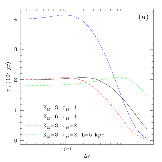
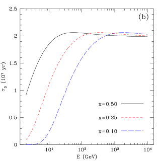
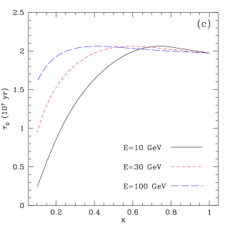
FIG. 1.: (a) The effective diffusion time $\tau_{D}$ as a function of $\Delta v$. When doubling the diffusion constant $K_{27}$, positrons remain trapped for a shorter time before escaping the galaxy. At low energy losses (small $\Delta v$) this of no importance since it is the energy loss time that is important in that region. When doubling the energy loss time $\tau_{16}$ we increase the flux at low energy losses since the positrons don’t lose energy as quickly. At higher energy losses, the flux goes down since the positrons have now had more time to escape. Increasing $L$ to 5 kpc, we see that diffusion becomes effective at a larger $\Delta v$, as expected. The positrons require more time to escape the larger diffusion region. The $10\%$ difference at low $\Delta v$ is because the function $f(r)$ depends on $L$. In (b) we show the effective diffusion time $\tau_{D}(xE,E)$ versus the injection energy $E$ for $x$=0.50, 0.25 and 0.10. In (c) we show the effective diffusion time $\tau_{D}(xE,E)$ as a function of $x$ for different injection energies. In (b) and (c) propagation model B is used.

The positron spectrum is now given by

$$\frac{dn}{d\varepsilon}=n_{0}^{2}\langle\sigma v\rangle_{\rm tot}\varepsilon^{-2}\int_{\varepsilon}^{\infty}d\varepsilon^{\prime}\,\frac{d\phi}{d\varepsilon^{\prime}}\tau_{D}\left[\varepsilon,\varepsilon^{\prime}\right],$$ (30)

giving the total positron spectrum

$$\frac{dn}{d\varepsilon}=n_{0}^{2}\langle\sigma v\rangle_{\rm tot}\varepsilon^{-2}\Bigg{\{}B_{\rm line}\tau_{D}\left[\varepsilon,{\tilde{m}_{\chi}}\right]+\int_{\varepsilon}^{{\tilde{m}_{\chi}}}d\varepsilon^{\prime}\,\left.\frac{d\phi}{d\varepsilon^{\prime}}\right|_{\rm cont.}\tau_{D}[\varepsilon,\varepsilon^{\prime}]\Bigg{\}}\theta\left({\tilde{m}_{\chi}}-\varepsilon\right).$$ (31)

Remembering that this is an expression for the number density of positrons, the flux is given by

$$\frac{d\Phi}{d\varepsilon}=\frac{\beta c}{4\pi}\frac{dn}{d\varepsilon}\simeq\frac{c}{4\pi}\frac{dn}{d\varepsilon},$$ (32)

where $\beta c$ is the velocity of a positron of energy $\varepsilon$. For the energies we are interested in, $\beta c\simeq c$ is a very well justified approximation.

We find that it is numerically advantageous to perform the integral in the variable $v$. Replacing the Jacobian factor, we find

$$\frac{dn}{d\varepsilon}=n_{0}^{2}\langle\sigma v\rangle_{\rm tot}\varepsilon^{-2}\Bigg{\{}B_{\rm line}\tau_{D}\left[\varepsilon,{\tilde{m}_{\chi}}\right]+\int_{v({\tilde{m}_{\chi}})}^{v(\varepsilon)}dv^{\prime}\,w(v^{\prime})\left.\frac{d\phi}{d\varepsilon}\right|_{\rm cont.}[\varepsilon(v^{\prime})]\tau_{D}[\varepsilon,\varepsilon(v^{\prime})]\Bigg{\}}\theta\left({\tilde{m}_{\chi}}-\varepsilon\right).$$ (33)

The function $\tau_{D}=\tau_{E}{\cal I}$ can be tabulated once. The integrand is smooth, and is thus easily computed for a range of values, equally spaced in $\ln\Delta v$. Likewise the sum on error functions converges rapidly, and for the range of $\Delta v$ values we are concerned with, need not be taken past $n=\pm 10$.

B Solar modulation

The formalism developed above gives the interstellar flux of positrons from neutralino annihilations. There is a further complication in that interactions with the solar wind and magnetosphere alter the spectrum. These effects are referred to as solar modulation. This can be neglected at high energies, but at energies below about 10 GeV, the effects of solar modulation become important. We will not consider solar modulation, since its effects can be removed by considering the positron fraction, $e^{+}/(e^{+}+e^{-})$, instead of the absolute positron fluxes.

However, another complication is the possibility that the solar modulation is charge-sign dependent as indicated in Ref. [22]. Following their treatment we can write the positron fraction at Earth in a solar cycle $A^{+}$ and $A^{-}$ respectively as

$$f^{+}_{E} = \frac{f^{2}(R+1)-f}{R(2f-1)},$$ (34)

$$f^{-}_{E} = \frac{f^{2}(R+1)-fR}{2f-1}.$$ (35)

where $f$ is the interstellar positron fraction and $R$ is the ratio of the total flux of positrons and electrons in a solar $A^{+}$ cycle to that in an $A^{-}$ cycle. The value $R$ can be measured, and is approximately given by [22]

$$R(\varepsilon)=\max\left[\min\left(0.45+0.17\;\ln\varepsilon,1\right),0.18\right].$$ (36)

We notice that in the absence of charge-sign dependence, the positron fraction is unaffected by solar modulation effects. As we will see later, the charge-sign dependent solar modulation worsens the agreement between the measurements and the expected background and given the large uncertainties involved, we will not use these expressions when predicting the positron fraction from neutralino annihilation.

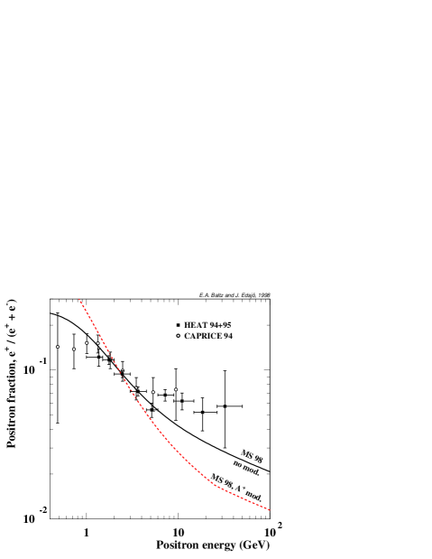
FIG. 2.: The positron fraction for the background is shown both without and with charge-sign dependent solar modulation [22]. The normalization has been kept free and is fitted to the Heat 94+95 data [23]. Also shown is the Caprice 94 data [24]. The backgrounds are parameterizations to the results by MS [25].

C Positron and electron backgrounds

When we want to compare our predictions with experiments, we must consider the expected background of positrons. Since most experiments measure the positron fraction and not the absolute positron flux, we also need to consider the electron background. We will use the most recent calculation by Moskalenko and Strong [25] (hereafter MS). For their model 08-005 without reacceleration, we have parameterized their calculated primary electron and secondary electron and positron fluxes as follows:

$$\left(\frac{d\Phi}{dE}\right)_{{\rm prim.~{}}e^{-}~{}\rm bkg} = \frac{0.16\,\varepsilon^{-1.1}}{1+11\,\varepsilon^{0.9}+3.2\,\varepsilon^{2.15}}\;{\rm GeV}^{-1}\;{\rm cm}^{-2}\;{\rm s}^{-1}\;{\rm sr}^{-1},$$ (37)

$$\left(\frac{d\Phi}{dE}\right)_{{\rm sec.~{}}e^{-}~{}\rm bkg} = \frac{0.70\,\varepsilon^{0.7}}{1+110\,\varepsilon^{1.5}+600\,\varepsilon^{2.9}+580\,\varepsilon^{4.2}}\;{\rm GeV}^{-1}\;{\rm cm}^{-2}\;{\rm s}^{-1}\;{\rm sr}^{-1},$$ (38)

$$\left(\frac{d\Phi}{dE}\right)_{{\rm sec.~{}}e^{+}~{}\rm bkg} = \frac{4.5\,\varepsilon^{0.7}}{1+650\,\varepsilon^{2.3}+1500\,\varepsilon^{4.2}}\;{\rm GeV}^{-1}\;{\rm cm}^{-2}\;{\rm s}^{-1}\;{\rm sr}^{-1}$$ (39)

where we as before have used $\varepsilon=E/(1~{}{\rm GeV})$. These parameterizations agree with their curves to within 10–15% for the whole intervals given in Ref. [25] (approximately 0.001–1000 GeV for primary electrons and 0.01–100 GeV for the secondary electrons and positrons). The parameterizations also have the same asymptotic slopes as the calculated fluxes at both the low and high energy end and extrapolations should be acceptable if not too far out of the regions given above. These predictions also agree roughly with the absolute flux measurements by the Heat experiment [26]. The experimental error bars are however smaller on the measurements of the positron fraction and in Fig. 2 we have made a fit to the Heat 94+95 measurements [23] of the positron fraction from the background alone keeping only the normalization of the positron flux free. We also show the best fits with charge-dependent solar modulation included. The normalization factors for the best fits are $k_{b}=1.11$ and $k_{b}=0.609$ without charge-dependent solar modulation and with $A^{+}$ modulation respectively ($A^{+}$ is the correct state for the Heat measurement). The corresponding reduced $\chi^{2}$ are 3.14 and 10.8, i.e. not very good fits. We also show the Caprice 94 measurements of the positron fraction [24].

We clearly see that the background is too steep at low energies and including the charge-sign dependent solar modulation only worsens the fit. For models with reacceleration, the fit is worse still[25]. We also note that there is an indication in the Heat data of an excess at 6–50 GeV. However, one should keep in mind that (a) the uncertainties below 10 GeV are large due to our poor knowledge of the solar modulation effects, (b) it is possible to make a better fit by hardening the interstellar nucleon spectrum [25] (even though this might be in conflict with antiproton measurements above 3 GeV[27]) and (c) it is possible to make a better fit by hardening the primary electron spectrum (even though this might be in conflict with direct electron measurements at higher energies [25]). We will not consider these issues here. Instead we will assume the background as given by the parameterizations above without charge-dependent solar modulation. We will then compare the positron background with our predictions and we also make a simultaneous fit of the positron fraction background signal from neutralino annihilations having only the normalization of the background and signal positron fluxes as free parameters.

To conclude the discussion of the backgrounds, there is clearly room (or even an indication) of an excess of positrons at intermediate energies that might be due to neutralino annihilations. However, the uncertainties are large and other explanations are feasible. We will entertain the possibility that the excess is due to neutralino annihilation in the next section.

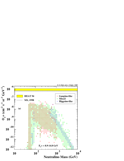
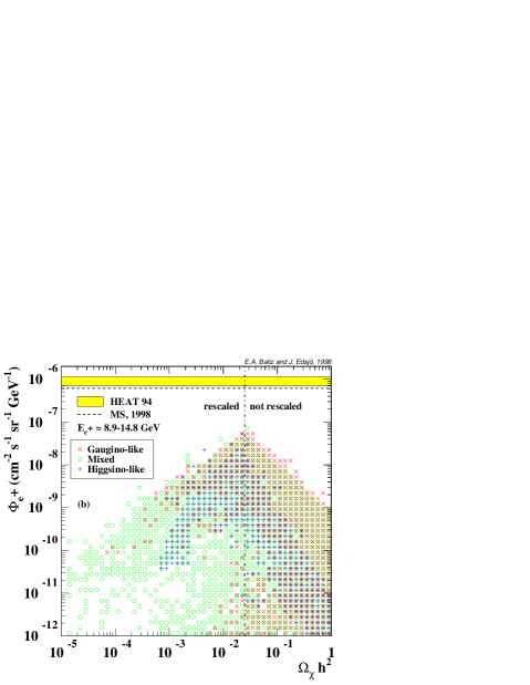
FIG. 3.: The flux of positrons from neutralino annihilation in the halo versus (a) the neutralino mass and (b) the neutralino relic density $\Omega_{\chi}h^{2}$. In (a) only models with $0.025<\Omega_{\chi}h^{2}<1$ have been included and in (b) models with $\Omega_{\chi}h^{2}<0.025$ have been rescaled by $(\Omega_{\chi}h^{2}/0.025)^{2}$. The Heat 94 data in this energy interval is shown together with the background prediction by MS [25] (as given by our parameterization, Eq. (39)).

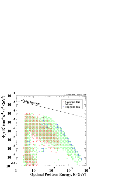
FIG. 4.: The flux of positrons, $\Phi_{e^{+}}E^{3}$ versus the optimal positron energy, $E$, for which the ratio of the signal flux to the background flux is highest. The positron background from MS [25] (as given by our parameterization, Eq. (39)) is shown as the dashed line. Above 100 GeV, the background is an extrapolation of the results by MS.

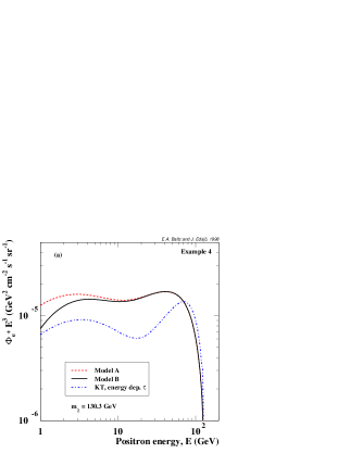
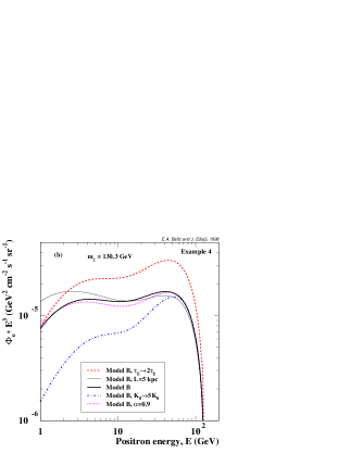
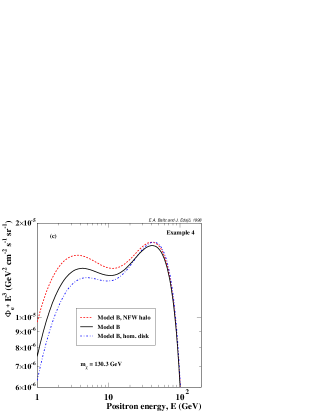
FIG. 5.: An example of a light model annihilating mainly into $W^{+}W^{-}$. In (a), the differences between our models A and B and the KT model with energy dependent escape time [6] are shown. In (b) the effects (for model B) of increasing $K$, $\tau_{E}$, $\alpha$ and $L$ are given and in (c), the differences between different halo profiles are shown. Note that the scale is different in (c).

		Parameters and units							$\chi$ properties
Example	Model	$\mu$	$M_{2}$	$\tan\beta$	$m_{A}$	$m_{0}$	$A_{b}/m_{0}$	$A_{t}/m_{0}$	$m_{\chi}$	$Z_{g}$	$\Omega_{\chi}h^{2}$
number	number	GeV	GeV	1	GeV	GeV	1	1	GeV	1	1
1	JE28__005683	$-852.3$	$-670.1$	13.1	664.0	1940.6	$-1.56$	$-1.60$	335.7	0.9951	0.029
2	JEsp3_000426	2319.9	4969.9	40.6	575.1	2806.6	2.0	0.27	2313.3	0.028	0.16
3	JE29__034479	$-1644.3$	$-202.2$	54.1	181.7	2830.9	2.57	2.50	101.6	0.99927	0.042
4	JE23__000159	$-221.8$	$-324.5$	1.01	792.2	2998.7	1.71	0.67	130.3	0.660	0.058

TABLE II.: Example models. The parameter values are given together with the neutralino masses, gaugino fractions and relic densities.

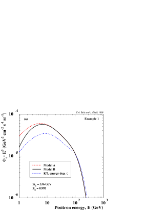
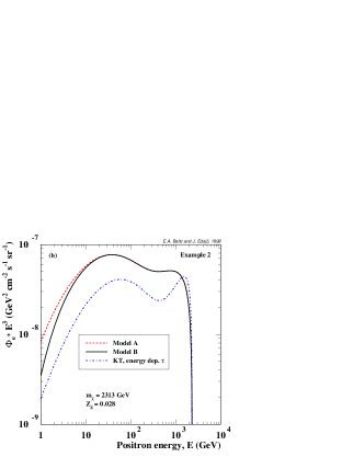
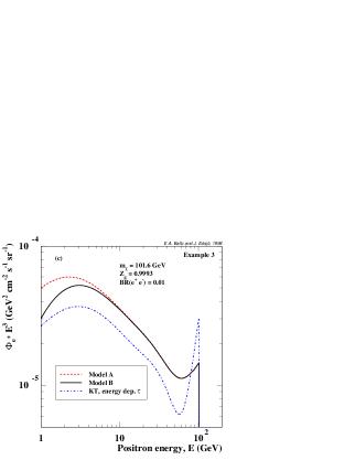
FIG. 6.: Example of positron spectra versus the positron energy. In (a) we show a typical spectrum for medium-heavy neutralinos, in (b) we show a spectrum from a heavy neutralino when gauge bosons dominate the annihilation final states and in (c) a spectrum when the branching ratio for annihilation into $e^{+}e^{-}$ has been increased to 0.01. In all spectra we show them as calculated with our two models and with the energy-dependent model by KT [6]

V Results

We are now ready the present our results and compare with the expected background and experimental measurements. We will first consider the absolute fluxes and investigate the dependence on the propagation parameters. We will use our propagation model B with the isothermal sphere as our default model. We will also show some typical spectra. In the next subsection we will then discuss the predicted positron fractions and compare with the experiments, in particular the excess at 6–50 GeV indicated by Heat data [23].

A Absolute fluxes and spectra

As a representative energy we will choose the average flux in the energy range 8.9–14.8 GeV which corresponds to one Heat bin (with average energy of about 11 GeV). In this energy range, we should be fairly unaffected by solar modulation effects. In Fig. 3 we show the absolute positron flux for propagation model B versus the neutralino mass and versus the relic density $\Omega_{\chi}h^{2}$. We also compare with the Heat 1994 measurement of the absolute flux [26]. We clearly see that with our canonical halo model we find no models that give fluxes as high as those measured. However, one should keep in mind that we probably have an overall uncertainty of about an order of magnitude coming from uncertainties regarding the propagation. We also have uncertainties coming from our lack of knowledge of the halo structure. For example, the halo could be clumpy which could easily increase the signal by orders of magnitude [28, 29]. The local halo density is also uncertain by at least a factor of 2 (which corresponds to a factor of 4 uncertainty in the positron flux). In Fig. 3 (a) we see that once we are above the $W$ mass, the spread of the predictions is much smaller. We also see that for heavy neutralinos, Higgsinos and mixed neutralinos typically give higher fluxes than the gaugino-like neutralinos. This is because the annihilation cross section to gauge bosons is very suppressed for gaugino-like neutralinos. For Higgsinos, the cross section to gauge bosons is also suppressed, but usually dominates anyway.

In Fig. 3 (b) we see that the highest fluxes are approximately proportional to $1/\Omega_{\chi}h^{2}$. This is because $\Omega_{\chi}h^{2}$ is approximately proportional to $\langle\sigma v\rangle^{-1}$ where $\langle\sigma v\rangle$ is the thermally averaged annihilation cross section. The highest fluxes for a given $\Omega_{\chi}h^{2}$ are obtained when the annihilation proceeds mainly to channels giving high positron fluxes and the velocity dependence of the cross section is small (i.e. the thermally averaged cross section is close to the annihilation cross section at rest). In that case, it is essentially the same cross section that determines both $\Omega_{\chi}h^{2}$ and the positron fluxes and hence the strong (anti)correlation. When $\Omega_{\chi}h^{2}<0.025$ we rescale the flux by $(\Omega_{\chi}h^{2}/0.025)^{2}$ and hence the fluxes for low $\Omega_{\chi}h^{2}$ are proportional to $\Omega_{\chi}h^{2}$. Note that in all other figures, we will only show the models where $0.025<\Omega_{\chi}h^{2}<1$.

In Fig. 4 we show the positron flux versus the optimal positron energy, $E_{e^{+}}^{\rm opt}$, where we define $E_{e^{+}}^{\rm opt}$ as the energy at which $(d\Phi/dE)_{\rm signal}/(d\Phi/dE)_{\rm background}$ is maximal. We also show the positron background prediction by MS [25]. We see that in many cases it is advantageous to look at higher energies than present experiments do. Again, we see that for heavier neutralinos, the mixed and Higgsino-like neutralinos give the highest fluxes.

In Fig. 5 we show an example of a spectrum when the neutralino mainly annihilates into $W^{+}W^{-}$. This model is example 4 in Table II. We choose this model as an example to explore the dependence of parameters and propagation models since it has two nice bumps from both primary as well as secondary and higher decays/hadronizations of the $W$ bosons. In (a) we compare our model A and B with the propagation model of KT [6] with energy dependent escape time. Compared to our model B, the KT propagation model assumes (i) that the diffusion constant coefficient $\alpha=1$, (ii) that there is no low energy cutoff of the diffusion constant (i.e. as our model A), (iii) that the energy-loss time $\tau_{E}$ is higher, (iv) that the diffusion constant $K_{0}$ is higher and (v) that the disk is homogeneous. They also use a leaky-box model instead of a diffusion model.

In Fig. 5 (a), we see that our model A gives higher fluxes than model B below about 10 GeV. This is easy to understand since model A has a lower diffusion constant at low energies and hence the positrons stay around longer and we get higher fluxes. On the other hand, the KT propagation gives a sharper peak from the primary decay of $W^{+}$ to $e^{+}$. This is, as we will see in figure (b) and (c), due to the different values of $K_{0}$, $\tau_{E}$ and $\alpha$. At low energies, the KT model has about the same shape as our model A, since neither $\tau_{E}$ nor the exact value of $\alpha$ are of big importance there. The different normalizations at low energies are due to different values of $K_{0}$.

In Fig. 5 (b) we show what happens in model B if we change the value of $K_{0}$, $\tau_{E}$, $\alpha$ or $L$. Increasing $K_{0}$ reduces the flux at lower energies (where diffusion is important), whereas increasing $\tau_{E}$ increases the flux at higher energies (where energy-loss is more important than escape through diffusion). We actually saw this behavior already in Fig. 1 (a) where $\tau_{D}$ was shown versus $\Delta v$ for different values of $K_{0}$ and $\tau$. Increasing $\alpha$ essentially tilts the spectrum clockwise at lower energies where diffusion is important. Hence, the dip at intermediate energies is more pronounced. Increasing $L$ has more or less the same effect as lowering $K_{0}$, except at higher energies, where we see a decrease in the flux. This is merely an artifact of the averaging over $z$ in Eq. (20). When $L$ increases, the average at a given $r$ decreases. We saw this behavior earlier in Fig. 1 (a).

In Fig. 5 (c) we show the dependence on the actual halo profile. We expect to mainly see the positrons that are created within a few kpc of us, but as we go lower in energy (and hence higher in energy loss), the visible region expands. In (c) we show the difference between the isothermal sphere and a homogeneous disk. The isothermal sphere gives higher fluxes at low energies, i.e. we see the galactic core at lower energies. If we use a steeper halo profile like the Navarro, Frenk and White profile [21], the flux at lower energies goes up even more. The dependence on the precise form of the halo profile is never very large though. It is mostly the propagation parameters that determine the shape of the spectrum.

To conclude, the differences between our models and the KT propagation model are mainly a matter of different parameters.

In Fig. 6 we show some other typical spectra (examples 1–3 in Table II). In (a) we show a spectrum when gauge bosons don’t dominate in the final state. In this case, we typically get a big wide bump without any special features. In (b), we show a spectrum for a heavy neutralino annihilating into gauge bosons. As in Fig. 5, we see two bumps from the decay of the $W$s. The right one comes from direct decay to $e^{+}$ and occurs at approximately $m_{\chi}/2$. The left one comes from secondary decays of $W$s, $W^{+}\to\tau^{+}(\mu^{+})\to e^{+}$ and positrons from quark jets, $W^{+}\to\cdots\to\pi^{+}\to e^{+}$. This bump occurs at approximately $m_{\chi}/60$. Exactly where the bumps occur depend on the propagation model used. In (c), we show a spectrum of a light neutralino where we have artificially boosted the branching ratio for direct annihilation into $e^{+}e^{-}$ to 1%. Typically this branching ratio is below $10^{-7}$, but if we e.g. have a large mass splitting of the selectrons, i.e. $m_{\tilde{e}_{1}}\gtrsim m_{\chi}$ and $m_{\tilde{e}_{2}}\gg m_{\chi}$ we can find mostly gaugino-like, but also some mixed models with a branching ratio $B_{e^{+}e^{-}}\gtrsim 0.01$. In this case, the line from monochromatic positrons might be visible and not too widened by propagation. We find that it is only when the branching ratio into $e^{+}e^{-}$ directly is reasonably high ($\gtrsim 0.001$) that the line is visible. We remark that if selectrons and smuons mix, the selectron degeneracy must be less than a few percent to avoid constraints from $\mu\rightarrow e\gamma$ [30, 1], though our model is allowed if the mixing between selectrons and smuons is negligible.

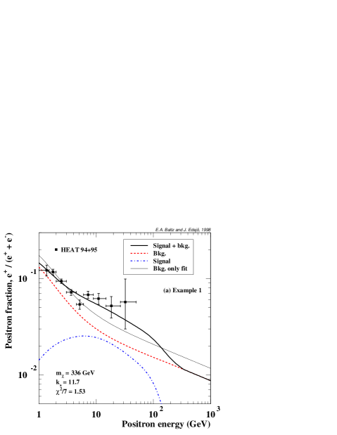
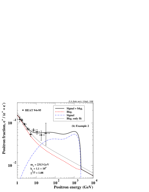
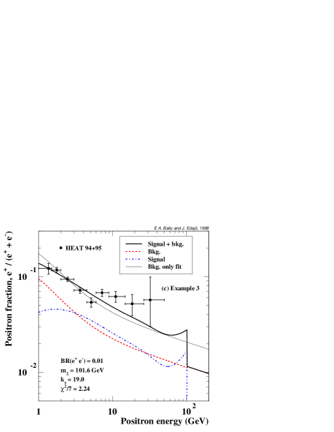
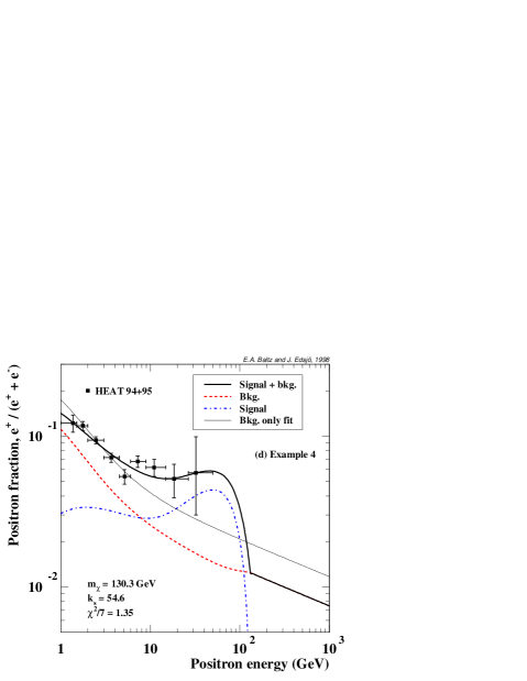
FIG. 7.: Example of positron fractions versus the positron energy. We show both the signal and background for the best simultaneous fit and also the best fit of the background alone. In (a) we show a typical spectrum for medium-heavy neutralinos, in (b) we show a spectrum for a heavy neutralino when gauge bosons dominate the annihilation final states, in (c) a spectrum when the branching ratio for annihilation into $e^{+}e^{-}$ has been increased to 0.01 and in (d) a spectrum from a medium-heavy neutralino when $W$s dominate.

B Positron fractions

Instead of comparing with the absolute fluxes, we will now compare with the measurement of the positron fraction by the Heat experiment [23]. As we saw in Fig. 2, the standard background predictions fail to reproduce the observations for all energies. Note, however, that the fit can be made better by adopting either a harder electron primary spectrum or a harder interstellar nucelon spectrum [25, 27]. A harder electron spectrum seems to be in disagreement with high-energy electron measurements [25] and a harder nucleon spectrum might be in contradiction with antiproton measurements above 3 GeV [27]. In light of this, it is therefore interesting to investigate if the possible excess at 6–50 GeV in the Heat data can be explained by neutralino annihilations in the halo. Note, however, the the uncertainties in the solar modulation (even though the charge-dependent solar modulation seems to worsen the fit) are large and not well understood.

We will in the following entertain the possibility that the standard prediction of the background is correct (to within a normalization) and make a simultaneous fit of the normalization of the background and the signal. We will not include the charge-dependent solar modulation. A study of the Heat data in terms of primary sources from WIMP annihilations has previously been performed in Ref. [31] where the KT results (both with and without energy-dependent escape time) were used.

We will compare with the most recent Heat measurement of the positron fraction (1994 and 1995 combined data) [23]. The error bars are smaller and the data cleaner for the positron fraction measurements. The Heat Collaboration gives their results in 9 bins from 1.0 to 50.0 GeV.

As we saw in Fig. 3 (a), the positron fluxes are typically an order of magniture or more smaller than the Heat measurements, and we find that we need to boost the signal by a boost factor, $k_{s}$, between 6 and $10^{10}$ to obtain a good fit. $k_{s}=10^{10}$ is hardly realistic, but $k_{s}$ up to 100–1000 might be acceptable given the uncertainties in both propagation and halo structure (the halo could e.g. be clumpy [28, 29]).

In Fig. 7 we show some examples of our positron fractions compared with the Heat measurements. The examples are the same as those shown earlier for the absolute fluxes, i.e. examples 1–4 in Table II. The signals have been boosted by the boost factors given by the best fit. Almost all of our models have the general feature of increasing the flux at intermediate energies as shown in (a). For some models, where the annihilation predominantly occurs to gauge bosons, we also expect a peak at roughly $m_{\chi}/2$ as shown in (b). The most pronounced feature, however, is the positron line. Even though smeared by propagation and energy loss, we still expect a sharp peak at $m_{\chi}$ if the branching ratio for annihilating into monochromatic positrons is high enough. However, the branching ratio is typically less than $10^{-7}$ and the feature is buried in the background. If the branching ratio is higher, the feature would be very clear as seen in (c). This might happen if there is a large mass splitting of the selectrons as discussed earlier. In (d) we show a light model annihilating mainly into gauge bosons and as seen, the bump from primary decay $W^{+}\to e^{+}$ can be made to fit the excess quite nicely.

In Ref. [31] models were found where the low-energy bump from gauge bosons can fit the excess at 6–50 GeV (as in our Fig. 7 (c)) without having to go to $\gtrsim$ 1 TeV neutralinos. They get better fits for lower masses than we do because they use the KT propagation model [6] which doesn’t shift features down in energy as much as our propagation does.

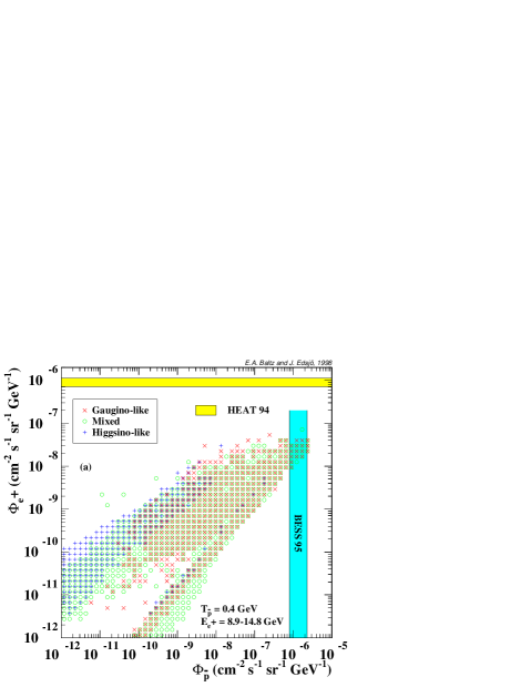
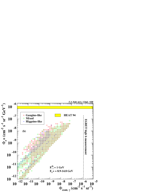
FIG. 8.: The flux of positrons versus that of (a) antiprotons and (b) continuum gammas. The experimental limits from Bess 95 [32] and high-altitude Egret [33] measurements are shown.

C Comparison with other signals

We have seen that the positron fluxes are typically at least factors of a few too low to be observable. However, with only a small amount of boosting of the signal (coming either from different propagation models and/or clumping of the dark matter) we obtain positron fluxes that can either roughly fit the indication of an excess seen in the Heat data or produce features possible to observe with future experiments. We must be concerned with other signals that might be boosted at a similar level and that might be in conflict with current observations.

In Fig. 8 we show the absolute flux of positrons versus the flux of (a) antiprotons [34, 29] and (b) continuum gammas [29]. The antiproton measurement of the Bess collaboration [32] is shown as well as the limit of the high galactic altitude diffuse gamma emission as measured by Egret [33]. We see that especially the antiprotons are expected to give about the same or better constraints on neutralino dark matter than the positrons. For the models with reasonable boost factors ($\lesssim$100–1000) the antiproton flux is usually about a factor of 1–10 closer to the experimental bound than the positrons. We might therefore worry about getting antiproton fluxes that are too large when boosting the positron fluxes. However, even though a factor of 10 might seem to be high, we have large uncertainties involved in the propagation and solar modulation. For the positrons we also have large uncertainties from the energy loss that don’t enter in the antiproton propagation. Changes in the diffusion constant also affect the positron and antiproton fluxes differently. Increasing $K_{0}$, the positron fluxes at higher energies are mainly unchanged (see Fig. 5 (b)), whereas the antiproton fluxes decrease. We also tend to sample a larger volume for antiprotons than we do for positrons and different halo profiles and clumpiniess hence enter differently for antiprotons and positrons. A factor of 10 difference is thus probably within the uncertainties.

For our examples and boost factors in Fig. 7, the corresponding maximal boost factors that would not violate the Bess upper limit [32] of $2.3\times 10^{-6}$ GeV^-1 cm^-2 s^-1 sr^-1 on the antiproton flux would be $k_{\bar{p}}$ = 9.8, $3.5\times 10^{5}$, 3.2 and 10.7. Compare this with the boost factors from our best fits to the Heat data, $k_{s}$ = 11.7, $1.1\times 10^{4}$, 19.0 and 54.6. The last two examples, Fig. 7 (c) and (d) have boost factors which contradicts the antiproton measurements by a factor of 5–6 but as explained above, the uncertainties are large and we prefer to keep these kind of models anyway.

The continuum gammas are very well correlated with the positron fluxes and of the same order of magnitude below present limits. The continuum gamma fluxes don’t suffer from large propagation uncertainties, but do depend more on the actual halo profile.

To conclude, it is intriguing that both the positron, antiproton and continuum gamma fluxes for our canonical halo and propagation models end up reasonably close to the observed fluxes. The correlation is also quite good, even though different uncertainties enter in all three different predictions.

Other signals, like direct detection of neutralinos and indirect detection from high-energy neutrinos from annihilation in the Sun/Earth are not affected by clumpiness to the same extent as the ones from halo annihilation. Both direct searches and neutrino telescopes have started cutting into the MSSM parameter space considered here. However, the limits are not completely watertight and we choose to keep all models even though some of our models might be excluded with typical assumptions about the halo density and velocity dispersion.

VI Conclusions

We conclude that for our canonical halo and propagation model, the positron fluxes from neutralino annihilation in the halo are lower than those experimentally measured. However, the predictions can easily be orders of magnitude too low due to our lack of knowledge of the structure of the halo (the halo could e.g. be clumpy). If we allow for this uncertainty we can easily obtain fluxes of the same order of magnitude as those measured. The shape of the signal spectrum is also different than the background and in most cases allows for a better fit of the excess at 6–50 GeV indicated by the Heat measurements than the background alone does.

If positrons from neutralinos make up a substantial fraction of the measured positron fluxes below 50 GeV, we usually have some features to search for at higher energies, especially if the annihilation occurs mainly to gauge bosons where we expect a clear bump at $m_{\chi}/2$. When the annihilation doesn’t go to gauge bosons, we only excpect a slight break in the spectrum at approximately $m_{\chi}/2$. This can be hard to find, unless we have detailed measurements around the break. If the branching ratio for annihilation into monochromatic positrons is higher than $\gtrsim 0.001$, as can happen if there is a pronounced mass splitting between selectrons, there is a very pronounced feature to search for at a positron energy of $m_{\chi}$.

We also note that our propagation models don’t preserve features as well as that of KT [6]. This is primarily due to the fact that KT uses an escape time that implies a larger diffusion constant. Features are also shifted to lower energies with our propagation models.

To conclude, there is a possibility to obtain measureable fluxes of positrons from neutralino annihilation in the Milky Way halo and they can easily be made to fit the excess indicated by Heat data. Future experiments will determine if there are features in the positron spectrum from neutralino annihilation.

- [1] G. Jungman, M. Kamionkowski and K. Griest, Phys. Rep. 267 (1996) 195.
- [2] See e.g. H.-U. Bengtsson et al., Nucl. Phys. B346 (1990) 129; V. Berezinsky et al., Phys. Lett. B325 (1994) 136; P. Chardonnet et al., Astrophys. J. 454 (1995) 774; See also Ref. [1] and references therein.
- [3] See e.g. P. Chardonnet, G. Mignola, P. Salati and R. Taillet, Phys. Lett. B384 (1996) 161; A. Bottino, F. Donato, N. Fornengo and P. Salati, astro-ph/9804137; See also Ref. [1] and references therein.
- [4] J. Silk and M. Srednicki, Phys. Rev. Lett. 53 (1984) 624; S. Rudaz and F. Stecker, Astrophys. J. 325 (1988) 16; J. Ellis, R.A. Flores, K. Freese, S. Ritz, D. Seckel and J. Silk, Phys. Lett. B214 (1989) 403; F. Stecker and A. Tylka, Astrophys. J. 336 (1989) L51.
- [5] M.S. Turner and F. Wilczek, Phys. Rev. D42 (1990) 1001; A.J. Tylka, Phys. Rev. Lett. 63 (1989) 840.
- [6] M. Kamionkowski and M. S. Turner, Phys. Rev. D43 (1991) 1774.
- [7] S. Ahlen et al. (Ams Collaboration), Nucl. Instrum. Methods A350 (1994) 351.
- [8] J. Edsjö and P. Gondolo, Phys. Rev. D56 (1997) 1879.
- [9] J. Edsjö, PhD Thesis, Uppsala University, hep-ph/9704384.
- [10] M. Drees, M.M. Nojiri, D.P. Roy and Y. Yamada, Phys. Rev. D56 (1997) 276; D. Pierce and A. Papadopoulos, Phys. Rev. D50 (1994) 565, Nucl. Phys. B430 (1994) 278; A.B. Lahanas, K. Tamvakis and N.D. Tracas, Phys. Lett. B324 (1994) 387
- [11] M. Carena, J.R. Espinosa, M. Quirós and C.E.M. Wagner, Phys. Lett. B355 (1995) 209.
- [12] Talk by J. Carr, March 31, 1998, http://alephwww.cern.ch/ALPUB/seminar/carrlepc98/index.html; Preprint ALEPH 98-029, 1998 winter conferences, http://alephwww.cern.ch/ALPUB/oldconf/oldconf.html.
- [13] M.S. Alam et al. (Cleo Collaboration), Phys. Rev. Lett. 71 (1993) 674; Phys. Rev. Lett. 74 (1995) 2885.
- [14] P. Gondolo and G. Gelmini, Nucl. Phys. B360 (1991) 145.
- [15] D.N. Schramm and M.S. Turner, Rev. Mod. Phys. 70 (1998) 303.
- [16] T. Sjöstrand, Comm. Phys. Comm. 82 (1994) 74; T. Sjöstrand, PYTHIA 5.7 and JETSET 7.4. Physics and Manual, CERN-TH.7112/93, hep-ph/9508391 (revised version).
- [17] L. Bergström, P. Ullio and J. Buckley, astro-ph/9712318.
- [18] L. Bergström and P. Ullio, Nucl. Phys. B504 (1997) 27.
- [19] W.R. Webber, M.A. Lee and M. Gupta, Astrophys. J. 390 (1992) 96.
- [20] M.S. Longair, High Energy Astrophysics, (Cambridge University Press, New York, 1994), Vol. 2, Chap. 19.
- [21] J.F. Navarro, C.S. Frenk and S.D.M. White, Astrophys. J. 462 (1996) 563.
- [22] J.M. Clem et al., Astrophys. J. 464 (1996) 507.
- [23] S.W. Barwick et al. (Heat Collaboration), Astrophys. J. 482 (1997) L191
- [24] G. Barbiellini et al. (Caprice Collaboration), Proceedings of 25th ICRC, Vol. 4, 213 (1997), Eds. M.S. Potgieter, B.C. Raubenheimer, D.J. van der Walt, Durban, South Africa.
- [25] I.V. Moskalenko and A.W. Strong, Astrophys. J. 493 (1998) 694.
- [26] S.W. Barwick et al. (Heat Collaboration), Astrophys. J. 498 (1998) 779.
- [27] I.V. Moskalenko, A.W. Strong and O. Reimer, astro-ph/9808084.
- [28] J. Silk and A. Stebbins, Astrophys. J. 411 (1993) 439.
- [29] L. Bergström, J. Edsjö, P. Gondolo and P. Ullio, astro-ph/9806072.
- [30] J. Ellis and D.V. Nanopoulos, Phys. Lett. B110 (1982) 44.
- [31] S. Coutu et al., Proceedings of 25th ICRC, Vol. 4, 213 (1997), Eds. M.S. Potgieter, B.C. Raubenheimer, D.J. van der Walt, Durban, South Africa.
- [32] A. Moiseev et al. (Bess Collaboration), Astrophys. J. 474 (1997) 479.
- [33] P. Sreekumar et al., Astrophys. J. 494 (1998) 523.
- [34] L. Bergström et al., work in progress.