Relativistic precession around rotating neutron stars: Effects due to frame-dragging and stellar oblateness

Abstract

General relativity predicts that a rotating body produces a frame-dragging (or Lense-Thirring) effect: the orbital plane of a test particle in a non-equatorial orbit precesses about the body’s symmetry axis. In this paper we compute the precession frequencies of circular orbits around rapidly rotating neutron stars for a variety of masses and equations of state. The precession frequencies computed are expressed as numerical functions of the orbital frequency observed at infinity. The post-Newtonian expansion of the exact precession formula is examined to identify the relative magnitudes of the precession caused by the Lense-Thirring effect, the usual Newtonian quadrupole effect and relativistic corrections. The first post-Newtonian correction to the Newtonian quadrupole precession is derived in the limit of slow rotation. We show that the post-Newtonian precession formula is a good approximation to the exact precession close to the neutron star in the slow rotation limit (up to $\sim 400$ Hz in the present context).

The results are applied to recent RXTE observations of neutron star low-mass X-ray binaries, which display kHz quasi-periodic oscillations and, within the framework of beat frequency models, allow the measurement of both the neutron star spin frequency and the Keplerian frequency of the innermost ring of matter in the accretion disk around it. For a wide range of realistic equations of state, we find that the predicted precession frequency of this ring is close to one half of the low-frequency ($\sim 20-35$ Hz) quasi-periodic oscillations seen in several Atoll sources.

1 Introduction

Neutron stars and black holes are the most compact objects, as such they provide an arena for the observation of strong gravitational effects predicted by the general theory of relativity. An important relativistic effect is the dragging of inertial frames, first predicted by Lense and Thirring (Lense and Thirring 1917). The Lense-Thirring frame dragging causes zero angular momentum observers (ZAMO’s) to orbit around a rotating body with non-zero angular velocity. If the orbit is inclined to the body’s equatorial plane, the plane of the orbit will precess. It has recently been noted (Stella and Vietri 1998a) that the precession frequency due to the frame-dragging effect has approximately the right magnitude and radial dependence to explain observations of accreting neutron stars made by the Rossi X-ray Timing Explorer (RXTE) satellite. If this interpretation is confirmed, it would provide a confirmation of the Lense-Thirring effect that includes its radial dependence, a test that is beyond reach of any other current or planned experiment to test frame dragging. The other interesting implication of this proposal is that it may be possible to constrain the neutron star’s equation of state, since the magnitude of the effect depends strongly on the star’s density profile. In order to determine whether the frame-dragging effect has been observed, the details of the dependence of the precession rate on position and the star’s mass, angular velocity and equation of state must be known. In this paper we will numerically compute the precession frequencies predicted by general relativity.

The magnitude of the Lense-Thirring effect increases with the rotating body’s angular momentum and compactness, so that it is largest for rapidly rotating neutron stars and black holes. However, the measurement of the frame-dragging due to the Earth’s motion appears to be within reach and several groups are actively pursuing this possibility. The Gravity Probe B experiment (Everitt et al. 1993 and references therein) is designed to measure the precession of gyroscopes in orbit around the Earth to an accuracy in the percent range, while a lower accuracy measurement of the Lense-Thirring precession of the orbit of the LAGEOS satellites has been reported (Ciufolini et al. 1998 and references therein). Both experiments are very difficult since the frame-dragging precession is many orders of magnitude smaller than the precession due to the Earth’s oblateness predicted by Newtonian gravity. The possibility of measuring frame-dragging due to the motion of neutron stars or black holes is attractive since the precession due to oblateness, while still important is smaller than the frame-dragging precession.

RXTE has recently discovered kilohertz quasi-periodic oscillations (kHz QPOs) in the X-ray light curves of over 15 accreting neutron stars in low mass X-ray binaries (see van der Klis 1998 for a review). This discovery is remarkable, since the dynamical frequency of a particle in circular orbit at radius $r\sim 6-8M$ (in geometric units G=c=1) is in the range of $1-1.5$ kHz for a $1.4M_{\odot}$ non-rotating neutron star. Thus, it is now possible to observe the region close to a neutron star where the gravitational field is strong and effects due to general relativity are important.

The X-ray observations have shown that the kHz QPO power spectrum peaks typically occur in pairs. The frequency of each QPO peak varies with time, often in response to X-ray flux, and therefore mass accretion rate, variations. However, in nearly all cases, the separation between the QPO peaks remains constant. A number of these neutron stars belong to the “Atoll” class and emit sporadic Type I X-ray bursts, likely originating from thermonuclear flashes in the freshly accreted material on their surface. RXTE revealed that during X-ray bursts an additional modulation of the X-ray flux is present, the frequency of which is consistent with either one or two times the kHz QPO peak separation frequency. These phenomena are most readily interpreted on the basis of the beat-frequency modulated accretion scenario originally suggested to interpret the lower frequency quasi periodic signals observed from accreting neutron stars and white dwarfs (see e.g. van der Klis 1995 and references therein). In beat frequency models the higher frequency kHz QPO peak corresponds to the orbital frequency of clumps of matter at the inner boundary of the accretion disk. The lower frequency kHz QPO peak is the beat frequency, corresponding to the difference between the clumps’ orbital frequency and the star’s spin frequency. This model naturally leads to the conclusion that the peak separation should be constant and equal to the star’s spin frequency. Application of the beat frequency model to the accreting neutron stars observed by RXTE indicates that they are spinning with periods close to $3ms$, although the modulation observed during some of type I X-ray bursts suggests that they might be spinning twice as fast.

Beat frequency models differ mainly with respect to the physical mechanism that determines the inner boundary of the accretion disk. This might be the presence of a neutron star magnetosphere (Alpar & Shaham 1985; Lamb et al. 1985), or the supersonic radial velocity of the disk material induced by radiation drag or the motion inside the innermost stable circular orbit, ISCO (Miller, Lamb & Psaltis 1998).

Another important aspect of the phenomenology of kHz QPO sources is that they display broad lower frequency QPO peaks, the frequency of which is correlated with the frequency of the kHz QPO peaks. In three “Atoll” sources $\sim 20-35$ Hz QPOs are observed; in the case of 4U1728-34 the frequency of these QPOs varies roughly with the square of the higher kHz QPO frequency (Stella and Vietri 1998a). In the higher luminosity “Z”-type sources GX5-1 and GX17+2 the frequency of the $\sim 15-60$ Hz “horizontal branch” QPOs appears also to depend quadratically on the frequency of the higher kHz QPOs (Stella and Vietri 1998a,b). It is this correlation between peaks which has suggested the following modification of the beat frequency model: if the star’s accretion disk is tilted with respect to the star’s equatorial plane, the orbital plane will precess due to the combined effect of frame-dragging and stellar oblateness. For orbits near a neutron star spinning with a period of $3ms$, the frame dragging effect is dominant and yields precession frequencies of a few tens of Hz which vary approximately as the square of the orbital frequency (Stella and Vietri 1998a). Close to the star the precession due to oblateness and other corrections due to general relativity will also be important and will cause departures from the quadratic scaling law. The principal purpose of this paper is to investigate in greater detail the precession frequency and its dependence on orbital frequency predicted by general relativity. This will provide a more accurate means of testing the precession hypothesis using many simultaneous observations of the QPO peaks in both the tens of Hz and kHz range.

QPO peaks have also been observed in X-ray binaries which probably contain black holes. It has been proposed that some of these QPO peaks also be identified with disk precession (Cui et al. 1998 and references therein). Rotating black holes are much simpler than neutron stars since their gravitational fields are completely specified by the Kerr geometry depending on only the hole’s mass and angular momentum. For this reason, measurements of precession near black holes have the potential to provide a much cleaner measurement of the Lense-Thirring effect. However, it should be noted that additional (kHz) QPO peaks corresponding to the $\phi$ and $\theta$ periodicities of spherical orbits have not yet been observed yet in black hole candidates, so that the precession hypothesis rests upon scarcer evidence and quantitative testing based on multiple QPO peaks is currently not a possibility. In any case, a thorough investigation of the precession of spherical orbits in the Kerr black hole geometry has been performed (Wilkins 1972, Merloni et al. 1998), so we will instead concentrate here on neutron star spacetimes.

In the calculations presented in this paper, it will be assumed that general relativity is the correct theory of gravity. The frame-dragging precession could hypothetically be used to test the validity of general relativity or other alternative theories of gravity using the parameterized post-Newtonian framework (Will 1993). However, the uncertainty in the equation of state for neutron stars would render it very difficult (or impossible) to differentiate between alternate theories of gravity.

We restrict our attention to the simplest possible model, a thin Keplerian disk tilted infinitesimally from the star’s equatorial plane. Both the corotating and counterrotating cases will be presented and discussed. Although this model may be oversimplified, it should suffice to capture the essential physical features of the problem and place accurate limits on the precession frequencies predicted by general relativity.

Accurate codes (Komatsu et. al. 1989, Cook et. al. 1992, Salgado et. al. 1994) now exist which can integrate the Einstein field equations for rapidly rotating neutron stars given a barotropic perfect fluid equation of state. Our method is to compute the spacetime metric of the neutron star using a code written by Stergioulas (1995) which is equivalent to Cook et. al.’s code and accurate to at least $1\%$ (Stergioulas and Friedman 1995, Nozawa et. al. 1998). The geodesic equations for test particles in the numerical spacetime can then be solved, yielding the orbital and precession frequencies.

The paper is organized as follows. In section  2 the predictions of general relativity regarding the orbital motion of a precessing test particle are reviewed and the numerical methods used to solve the characteristic frequencies are outlined. In section  3 an asymptotic expansion of the precession formula is derived in order to discuss the validity of the approximate Newtonian formula. The neutron star parameters which were selected are described in section  4. In section  5 general results are presented for a variety of equations of state, stellar masses and angular velocities. These results are compared with the power spectra of the LMXBs observed by RXTE. We find that for corotating orbits the observed precession frequencies are somewhat lower than predicted using the approximate method of Stella and Vietri (1998a), therefore increasing the discrepancy between the predicted precession frequency and the observations, especially for “Z”-type kHz QPO sources. These conclusions and their consequences are discussed in the final section.

2 Models of Rapidly Rotating Relativistic Neutron Stars

The neutron star models which we compute are assumed to be stationary, axisymmetric, uniformly rotating perfect fluid solutions of the Einstein field equations. The assumptions of stationarity and axisymmetry allow the introduction of two commuting Killing vectors $\phi^{\alpha}$ and $t^{\alpha}$, generating rotations and time-translations as well as coordinates $\phi$ and $t$, defined by the conditions (see eg., Friedman, Ipser and Parker, 1986)

$$t^{\alpha}\nabla_{\alpha}t=\phi^{\alpha}\nabla_{\alpha}\phi=1\;,\;t^{\alpha}\nabla_{\alpha}\phi=\phi^{\alpha}\nabla_{\alpha}t=0,$$ (1)

labeling the two-surfaces spanned by the Killing vectors. As a result, the metric, $g_{\alpha\beta}$ can be written as

$$ds^{2}=-e^{\gamma+\rho}dt^{2}+e^{\gamma-\rho}\bar{r}^{2}\sin^{2}\theta\left(d\phi-\omega dt\right)^{2}+e^{2\alpha}\left(d\bar{r}^{2}+\bar{r}^{2}d\theta^{2}\right),$$ (2)

where the metric potentials $\rho,\gamma,\alpha$ and $\omega$ depend only on the coordinates $\bar{r}$ and $\theta$. The function $\frac{1}{2}(\gamma+\rho)$ is the relativistic generalization of the Newtonian gravitational potential; the time dilation factor between an observer moving with angular velocity $\omega$ and an observer at infinity is $e^{\frac{1}{2}(\gamma+\rho)}$. The coordinate $\bar{r}$ is not the same as the Schwarzschild coordinate $r$. In the limit of spherical symmetry, $\bar{r}$ corresponds to the isotropic Schwarzschild coordinate. Circles centred about the axis of symmetry have circumference $2\pi r$ where $r$ is related to our coordinates $\bar{r},\theta$ by

$$r=e^{\frac{1}{2}(\gamma-\rho)}\bar{r}\sin\theta.$$ (3)

The metric potential $\omega$ is the angular velocity about the symmetry axis of ZAMOs and is responsible for the Lense-Thirring effect. The fourth metric potential, $\alpha$ specifies the geometry of the two-surfaces of constant $t$ and $\phi$. When the star is non-rotating, the exterior geometry is that of the isotropic Schwarzschild metric, with

$$e^{\frac{1}{2}(\gamma+\rho)}=\frac{1-M/2\bar{r}}{1+M/2\bar{r}},\;e^{\frac{1}{2}(\gamma-\rho)}=e^{\alpha}=\left(1+M/2\bar{r}\right)^{2},\;\omega=0.$$ (4)

We shall investigate uniformly rotating perfect fluid stars with stress tensor

$$T^{\alpha\beta}=(\epsilon+p)u^{\alpha}u^{\beta}+pg^{\alpha\beta}$$ (5)

where $\epsilon$ and $p$ are the fluid’s energy density and pressure as measured by a co-moving observer. The fluid four-velocity,

$$u^{\alpha}=u^{t}(t^{\alpha}+\Omega\phi^{\alpha}),$$ (6)

is a linear combination of the Killing vectors. The factor $u^{t}$ is a function of $r$ and $\theta$ specified by the condition that $u^{\alpha}$ is a unit, time-like vector, while $\Omega$ is the constant angular velocity of the star. We will numerically integrate the field equations by assuming various zero-temperature, barotropic equations of state of the form $\epsilon=\epsilon(p)$.

The numerical method used to integrate the Einstein field equations for the metric potentials is identical to the method described by Cook et. al. (1992 and corrections in 1994a) which is based on the self-consistent field method presented by Komatsu et. al. (1989). Since the method has been described in detail in these papers, we will only explicitly discuss aspects of the code which have direct bearing on the present work.

The field equations can be written in a form of a set of elliptic partial differential equations, which can be formally solved using a standard Green function approach (Komatsu et. al. 1989). As a result, the solution for the metric potentials $\nu,\beta$ and $\omega$ can be expressed as a series

$$\gamma(\bar{r},\theta) = -\frac{2}{\pi}e^{-\gamma/2}\Sigma_{n=1}^{\infty}\frac{\sin\left((2n-1)\theta\right)}{(2n-1)\sin\theta}\gamma_{n+1}(\bar{r})$$ (7)

$$\rho(\bar{r},\theta) = -e^{-\gamma/2}\Sigma_{n=0}^{\infty}P_{2n}(\cos\theta)\rho_{n+1}(\bar{r})$$ (8)

$$\omega(\bar{r},\theta) = -e^{\rho-\gamma/2}\Sigma_{n=1}^{\infty}\frac{P^{1}_{2n-1}(\cos\theta)}{2n(2n-1)\sin\theta}\omega_{n+1}(\bar{r})$$ (9)

where the expansion coefficients, given by integrals of the metric potentials over all of space are determined iteratively once an equation of state is specified. In the numerical implementation, the sums are taken only over a finite range and we keep only the first ten terms in the series. The fourth metric potential, $\alpha$ is determined by quadrature once the other potentials are known.

Once the geometry of the star is determined, the total mass, baryonic mass and angular momentum of the star, $M$, $M_{B}$ and $J$ respectively can be computed. This involves integration of the metric potentials and the stress tensor over all space (Komatsu et. al. 1989).

2.1 Geodesic Motion for Circular Orbits

The assumptions that the neutron star is stationary and axisymmetric has the consequence that two constants of motion are associated with any orbit, corresponding to the energy per unit mass, $E$, and orbital angular momentum per unit mass, $L$. As a result, the set of all circular orbits confined to the star’s equatorial plane is a two-parameter family depending only on $E$ and $L$, once the background metric is determined. The theory of these orbits and their perturbations is presented by Bardeen (1970, 1973). Bardeen introduces a one-parameter family of orbits corresponding to the motion of zero-angular momentum observers (ZAMOs) which have $L=0$. Although these observers have zero angular momentum, the dragging of inertial frames by the rotating star causes the ZAMOs to orbit the star with angular velocity $\omega$, as seen by an observer at infinity.

It is useful to consider the motion of other observers with reference to the ZAMOs. Consider a particle confined to a circular orbit in the star’s equatorial plane with four-velocity

$$U^{\alpha}:=\frac{dx^{\alpha}}{d\tau}=\left[\frac{dt}{d\tau}\right]_{\pi/2}\left(t^{\alpha}+\left[\frac{v_{\infty}}{r}\right]_{\pi/2}\phi^{\alpha}\right)$$ (10)

where $\tau$ is the particle’s proper time and $v_{\infty}$ is the particle’s physical three-velocity as measured by an observer at infinity. Square brackets with subscript $\pi/2$ denotes that the quantity within the brackets is evaluated in the star’s equatorial plane, $\theta=\pi/2$. The four-momentum per unit particle mass is

$$p_{\alpha}=g_{\alpha\beta}U^{\beta}=-E\nabla_{\alpha}t+L\nabla_{\alpha}\phi\;.$$ (11)

¿From the definition of four-momentum, the particle’s four-velocity is determined by $E$ and $L$ through the relations

$$\left[\frac{dt}{d\tau}\right]_{\pi/2} = \left[(E-\omega L)e^{-(\gamma+\rho)}\right]_{\pi/2}$$ (12)

$$\left[v_{\infty}\right]_{\pi/2} = \left[\omega r+\frac{L}{E-\omega L}\frac{e^{\gamma+\rho}}{r}\right]_{\pi/2}$$ (13)

A ZAMO will measure the particle to move with a velocity, $v$ defined by

$$\left[v\right]_{\pi/2}=\left[e^{-(\gamma+\rho)/2}(v_{\infty}-\omega r)\right]_{\pi/2}.$$ (14)

The constants of motion $E$ and $L$ can be rewritten explicitly in terms of $v$,

$$L = \left[\frac{vr}{\sqrt{1-v^{2}}}\right]_{\pi/2}$$ (15)

$$E-\left[\omega\right]_{\pi/2}L = \left[\frac{1}{\sqrt{1-v^{2}}}e^{\frac{1}{2}(\gamma+\rho)}\right]_{\pi/2},$$ (16)

where $(E-\omega L)\exp{-\frac{1}{2}(\gamma+\rho)}$ is the energy of the particle measured by a ZAMO. The solution of the geodesic equation yields two possible values for the three-velocity (Bardeen, 1970),

$$\left[v_{\pm}\right]_{\pi/2}=\left[\frac{e^{-\rho}\bar{r}^{2}\omega_{,\bar{r}}\pm\left(e^{-2\rho}\bar{r}^{4}\omega_{,\bar{r}}^{2}+2\bar{r}(\gamma_{,\bar{r}}+\rho_{,\bar{r}})+\bar{r}^{2}(\gamma_{,\bar{r}}^{2}-\rho_{,\bar{r}}^{2})\right)^{1/2}}{2+\bar{r}(\gamma_{,\bar{r}}-\rho_{,\bar{r}})}\right]_{\pi/2},$$ (17)

where $v_{+}$ and $v_{-}$ correspond to co-rotating and counter-rotating orbits respectively. The Kepler frequencies, $\nu_{K\pm}$ are defined as the orbital frequency of the prograde and retrograde circular orbits as measured by asymptotic observers

$$\nu_{K\pm}:=\left[\frac{v_{\infty\pm}}{2\pi r}\right]_{\pi/2}=\left[\frac{1}{2\pi}\left(v_{\pm}\frac{e^{\rho}}{\bar{r}}+\omega\right)\right]_{\pi/2}$$ (18)

2.2 Precession of Tilted Orbits

We now turn to circular geodesics which are not confined to the star’s equatorial plane. It is simplest to consider motion where the angle of inclination between the orbital and equatorial planes is infinitesimally small.

The four-velocity of a particle moving on a circular orbit inclined to the star’s equatorial plane is

$$U^{\alpha}=\frac{dt}{d\tau}\left(t^{\alpha}+\frac{v_{\infty}}{r}\phi^{\alpha}\right)+\frac{d\theta}{d\tau}\delta^{\alpha}_{\theta}\;.$$ (19)

The values of $\frac{dt}{d\tau}$ and $v_{\infty}$ on the star’s equatorial plane are given by Eqs. (12) and (13) respectively. The normalization condition $U^{\alpha}U_{\alpha}=-1$ leads to an equation for $\theta(\tau)$ which takes the form of particle motion in a one-dimensional potential,

$$0=\frac{1}{2}\left(\frac{d\theta}{d\tau}\right)^{2}+V(\theta)\;,$$ (20)

where the potential is (Bardeen, 1970)

$$V(\theta)=\frac{1}{2}\frac{e^{-2\alpha}}{\bar{r}^{2}}\left(-1+e^{-(\gamma+\rho)}(E-\omega L)^{2}+\frac{L^{2}}{\bar{r}^{2}\sin^{2}\theta}e^{\rho-\gamma}\right)\;.$$ (21)

Consider an orbit which only makes small oscillations out of the star’s equatorial plane. This orbit is defined by the conditions $\left[V(\theta)\right]_{\pi/2}=\left[\partial_{\theta}V\right]_{\pi/2}=0$. The first condition is automatically met by the assumed form of the four-velocity. The symmetry of the spacetime guarantees that the second condition is met. The frequency of the oscillation is given by

$$\left(d\theta/d\tau\right)^{2}=\left[\partial_{\theta}\partial_{\theta}V\right]_{\pi/2}\;.$$ (22)

The precession frequency $\nu_{p}$ of disk’s orbital plane about the star’s axis of symmetry is the difference between the frequency of oscillations of the particle in the longitudinal and latitudinal directions, $2\pi\nu_{p}:=d\phi/dt-d\theta/dt$, as observed by observers at infinity. The explicit formula is

$$2\pi\nu_{p\pm}=\left[\omega+\frac{v_{\pm}}{\bar{r}}e^{\rho}\left(1-e^{\alpha+\frac{1}{2}(\gamma-\rho)}X(r,\theta)\right)\right]_{\pi/2}$$ (23)

where $\nu_{p+}$ and $\nu_{p-}$ are the precession frequencies of prograde and retrograde orbits respectively, and the function $X(r,\theta)$ is defined by

$$X(r,\theta):=\left(1+\frac{1}{2}\partial_{\theta}\partial_{\theta}(\rho-\gamma)+\frac{1}{2v_{\pm}^{2}}\partial_{\theta}\partial_{\theta}(\rho+\gamma)+\frac{\bar{r}}{v_{\pm}}e^{-\rho}\partial_{\theta}\partial_{\theta}\omega\right)^{1/2}.$$ (24)

This formula is similar to the expression for the precession frequency derived by Ryan (1995) for orbits in a vacuum spacetime. Since Ryan assumes the spacetime is vacuum everywhere, his expression for the precession frequency does not include terms proportional to $\partial_{\theta}\partial_{\theta}\gamma$.

For slowly rotating stars with dimensionless rotation parameter $j=J/M^{2}\ll 1$, it is meaningful to split Eq. (23) into two terms, a precession frequency due to the Lense-Thirring effect,

$$\nu_{LT}=(\nu_{p+}+\nu_{p-})/2=\omega/2\pi+O(j^{3})$$ (25)

and a precession due to the star’s oblateness,

$$\nu_{oblate}=(\nu_{p+}-\nu_{p-})/2$$ (26)

which is the relativistic generalization of the Newtonian quadrupole precession. Thus, to leading order, the precession of orbits due to the L-T effect is equal to the orbital frequency of a ZAMO ($\omega/2\pi$) in an equatorial orbit around the star. It should be remembered, however, that the frame-dragging potential $\omega$ makes contributions to the velocity, $v_{\pm}$, and the frequency which we have named $\nu_{oblate}$. If the star is rotating rapidly, such a split may not be meaningful.

The precession frequency is easily computed once the metric expansion coefficients appearing in Eqs. (7) - (9) have been computed. The second partial derivative of the metric potentials are evaluated using standard relations for Legendre polynomials and trigonometric functions

$$\left[\partial_{\theta}\partial_{\theta}\gamma\right]_{\pi/2} = -\left[\frac{4}{\pi(2+\gamma)}e^{-\gamma/2}\right]_{\pi/2}\Sigma_{n=2}^{\infty}(-1)^{n}\left((2n-1)-\frac{1}{2n-1}\right)\gamma_{n+1}(r)$$ (27)

$$\left[\partial_{\theta}\partial_{\theta}\rho\right]_{\pi/2} = -\left[\frac{\rho\partial_{\theta}\partial_{\theta}\gamma}{2}\right]_{\pi/2}-\left[e^{-\gamma/2}\right]_{\pi/2}\Sigma_{n=1}^{\infty}(2n-1)(2n+1)P_{2n-2}(0)\rho_{n+1}(r)$$ (28)

$$\left[\partial_{\theta}\partial_{\theta}\omega\right]_{\pi/2} = \left[\omega\left(\partial_{\theta}\partial_{\theta}\rho-\frac{\partial_{\theta}\partial_{\theta}\gamma}{2}\right)\right]_{\pi/2}$$ (29)

$$-\left[e^{\rho-\frac{1}{2}\gamma}\right]_{\pi/2}\Sigma_{n=2}^{\infty}\left(\frac{1}{n}-(2n-1)\right)P_{2n-2}(0)\omega_{n+1}(r)\;.$$

3 Asymptotic Expansions

Our main interest in this paper is in the motion of test particles near a neutron star rotating arbitrarily quickly. The motion of a particle making small oscillations out of the star’s equatorial plane is determined exactly by the formulae presented in section 2, once the spacetime’s geometry has been determined numerically. Although, this method provides a sufficient description of the motion, it is useful to examine the weak field, slow rotation limit to elucidate the nature of the orbital precession. This corresponds to a double expansion in two small parameters, $M/r$ and $j:=J/M^{2}$, which isn’t generally a good description of the strong gravitational field near a rapidly rotating neutron star. However, from this double expansion, the Newtonian quadrupole formula will emerge, which will allow us to discuss the validity of the Newtonian formula.

Since the spacetime is asymptotically flat, the coefficients in the expansion of the metric potentials Eqs. (7) - (9) must decay at large $r$ as (Komatsu et. al. 1989)

$$\gamma_{n+1}(r)\sim\left(\frac{M}{r}\right)^{2n}\;,\;\rho_{n+1}(r)\sim\omega_{n+1}(r)\sim\left(\frac{M}{r}\right)^{2n+1}\;.$$ (30)

In the slow rotation approximation is an expansion in small $j$ with leading order behaviour of the coefficients given by

$$\gamma_{n+1}(r)\sim\rho_{n+1}(r)\sim j^{2n}\;,\;\omega_{n+1}(r)\sim j^{2n-1}\;.$$ (31)

Hartle’s (1967) slow rotation formalism is equivalent to keeping terms in the series expansions (7) - (9) up to and including $n=1$. The explicit form of the leading order coefficients have been calculated by Butterworth and Ipser (1976). Comparing with their work, we find the following dependencies at large $r$, keeping only the terms of lowest order in $j$,

$$\rho_{1}(\bar{r}) = \frac{2M}{\bar{r}}+\frac{B_{0}}{\bar{r}^{2}}\left(1+\frac{M}{3\bar{r}}\right)+O(1/\bar{r}^{4})$$ (32)

$$\rho_{2}(\bar{r}) = -2\frac{\Phi_{2}}{\bar{r}^{3}}+4\frac{J^{2}}{\bar{r}^{4}}+O(1/\bar{r}^{5})$$ (33)

$$\gamma_{2}(\bar{r}) = -\frac{\pi}{2}\frac{B_{0}}{\bar{r}^{2}}+O(1/\bar{r}^{3})$$ (34)

$$\omega_{2}(\bar{r}) = -4\frac{J}{\bar{r}^{3}}+O(1/\bar{r}^{4})$$ (35)

where $\Phi_{2}$ is the relativistic generalization of the Newtonian quadrupole moment (Butterworth and Ipser 1976; Ryan 1995; Laarakkers and Poisson 1997). We choose to define $\Phi_{2}$ so that it is positive for an oblate spheroid. The second term in Eq. (33) is the first post-Newtonian correction to the quadrupole moment. The constant $B_{0}$ is determined by an integral over the star given by Butterworth and Ipser (1976) (which they label $\tilde{B}_{0}$). Integration of the field equation for $\alpha$ at large $\bar{r}$ results in

$$\alpha+\frac{1}{2}(\gamma+\rho)=\frac{1}{\bar{r}^{2}}\left(-B_{0}-\frac{M^{2}}{2}+\cos^{2}\theta\left(2B_{0}+\frac{M^{2}}{2}\right)\right)+O(1/\bar{r}^{4})\;.$$ (36)

Substituting the asymptotic expansions (32) - (35) into Eq. (17), the particle velocity measured by observers at infinity is

$$v_{\infty\pm}=\pm\sqrt{\frac{M}{r}}-j\frac{M^{2}}{r^{2}}+O\left(j^{2}\left(\frac{M}{r}\right)^{5/2}\right).$$ (37)

The number of terms which must be included in this series depends on the relative size of the two expansion parameters. For $1.4M_{\odot}$ stars spinning at the rate observed by RXTE, ( $\sim$ 3 ms period), the rotation parameter $j\sim 0.1-0.2$ for equations of state from the Arnett and Bowers (1977) catalog (Cook et. al. 1994). For this range of rotation parameter, when $M/r<4/9$ the second term in Eq. (37) is at most a $6\%$ correction to the first term, which is the usual Kepler velocity for a non-rotating spacetime. However, if the star is rotating close to its maximum possible angular velocity, then the rotation parameter may approach unity (in fact there is no theoretical upper limit for $j$ as there is for black holes) and Eq. (37) will not be a good approximation for Eq. (14).

A weak field, slow rotation limit of the precession frequencies can be derived in the limit $j\left(M/r\right)^{3/2}\ll 1$. In this case, occurences of $v_{\pm}$ and $\bar{r}$ can be replaced by $\nu_{K}$ and the star’s mass, through the relation

$$\frac{ve^{\rho}}{\bar{r}}=2\pi\nu_{K}+O(j\left(\frac{M}{r}\right)^{3/2})=\sqrt{\frac{M}{r^{3}}}+O(j\left(\frac{M}{r}\right)^{3/2}).$$ (38)

In this limit, the Lense-Thirring precession frequency, Eq. (25) is

$$\nu_{LT}=\frac{8\pi^{2}I\nu_{s}\nu_{K}^{2}}{c^{2}M},$$ (39)

where factors of $G$ and $c$ have been restored and $\nu_{s}:=\Omega/2\pi$ is the spin frequency of the star.

The precession due to the star’s oblateness can be found by noting that in the weak field, slow rotation limit, the function $X$ appearing in Eq. (23) is

$$[X]_{\pi/2}=\left(1+{3}\frac{(v^{2}+1)}{v^{2}}\left(\frac{\Phi_{2}}{\bar{r}^{3}}-2\frac{J^{2}}{\bar{r}^{4}}\right)\right)^{1/2}.$$ (40)

Making use of the asymptotic expression Eq. (38) for $v$, the function $X$ reduces to

$$[X]_{\pi/2}=1+{3}\frac{e^{2\rho}r^{3}}{M\bar{r}^{2}}\left(1+\frac{M}{\bar{r}}\right)\left(\frac{\Phi_{2}}{\bar{r}^{3}}-2\frac{J^{2}}{\bar{r}^{4}}\right).$$ (41)

The expression for $\nu_{oblate}$ is then

$$\nu_{oblate} = \nu_{K}\left(1-e^{-\alpha+\frac{1}{2}(\gamma-\rho)}\right)$$ (42)

$$-3\nu_{K}\frac{e^{2\rho+\alpha+\frac{1}{2}(\gamma-\rho)}r^{3}}{M\bar{r}^{2}}\left(1+\frac{M}{\bar{r}}\right)\left(\frac{\Phi_{2}}{\bar{r}^{3}}-2\frac{J^{2}}{\bar{r}^{4}}\right).$$

At this level of approximation it is sufficient to use the values of $\bar{r},\rho,\gamma$ and $\alpha$ in spherical symmetry, given by Eqs. (3) and (4). The precession frequency due to the star’s oblateness can now be split into terms

$$\nu_{oblate}=\nu_{quad}\left(1+c_{PN}\frac{M}{r}\right)+\nu_{cent}.$$ (43)

In equation (43), $\nu_{quad}$ and $\nu_{cent}$ correspond to the the Newtonian quadrupole precession and a centrifugal precession due to other relativistic effects which enter at the same order as the Newtonian quadrupole term. The constant $c_{PN}$ is the coefficient of the first post-Newtonian correction to the Newtonian quadrupole precession. The Newtonian quadrupole precession is

$$\nu_{quad} = -\frac{3\nu_{K}}{2}\frac{\Phi_{2}}{Mr^{2}}$$ (44)

$$= -3\Phi_{2}\left(\frac{2\pi^{2}}{G^{2}M^{5}}\right)^{1/3}\nu_{K}^{7/3}.$$ (45)

The post-Newtonian correction parameter has the value

$$c_{PN}=3-2j^{2}\frac{M^{3}}{\Phi_{2}}\;.$$ (46)

For black holes $\Phi_{2}=\frac{G^{2}}{c^{4}}j^{2}M^{3}$, so that $c_{PN}=1$. However, for neutron stars this is not the case. It has been shown by Laarakkers and Poisson (1997) that $\Phi_{2}\simeq a(M,\hbox{EOS})\frac{G^{2}}{c^{4}}j^{2}M^{3}$ with $a(M,\hbox{EOS})$ a constant which depends on the star’s mass and equation of state. For EOS from the Arnett and Bowers (1977) catalogue, $a\sim 2-12$. The constants $a(M,\hbox{EOS})$ increase with decreasing mass for a fixed EOS, while they increase for increasing stiffness for fixed mass (Laarakkers and Poisson 1997). It follows that the first post-Newtonian correction term is most important for the stiffest equations of state and the smallest mass stars. At distances close to $6M$, the post-Newtonian correction term can correspond to as much as a $50\%$ correction to the quadrupole precession, and can’t be neglected.

The centrifugal precession frequency is defined by

$$\nu_{cent}:=\nu_{K}\left[\left(1-e^{-\alpha+\frac{1}{2}(\gamma-\rho)}\right)\right]_{\pi/2}\;.$$ (47)

The function $\left[1-\exp({-\alpha+\frac{1}{2}(\gamma-\rho)})\right]_{\pi/2}$ measures the fractional difference in the proper length elements of two infinitesimal curves, both centred about the same point on the star’s equatorial plane. The first curve is defined by constant values of the coordinates $\phi,\bar{r}$ and $t$, and has proper length $dl_{1}=\bar{r}\left[\exp\alpha\right]_{\pi/2}d\theta$. The second curve is restricted to the star’s equatorial plane and has proper length $dl_{2}=\bar{r}\left[\exp{\frac{1}{2}(\gamma-\rho)}\right]_{\pi/2}d\phi$. If the spacetime is spherically symmetric (or flat), the proper length of the two curves must agree and the frequency $\nu_{cent}$ vanishes. When the star is rotating, the proper lengths will not agree, but the condition of asymptotic flatness requires that their difference falls off at least as fast as $1/r^{2}$. Making use of the asymptotic expansions (32) - (36), the centrifugal precession frequency is

$$\nu_{cent}=-\nu_{K}\beta\left(\frac{M}{r}\right)^{2}$$ (48)

where the dimensionless constant $\beta$ defined by

$$\beta=\frac{1}{M^{2}}\left(2B_{0}+M^{2}/2\right)$$ (49)

is of order $j^{2}$ for slowly rotating stars. The percent magnitude of the centrifugal precession relative to the quadrupole precession is

$$\zeta:=\frac{\nu_{cent}}{\nu_{quad}}\times 100=\frac{200}{3}\beta\frac{M^{3}}{\Phi_{2}}$$ (50)

and is displayed in Tables 1 - 4. The size of this term relative to the quadrupole precession depends on the star’s mass and equation of state, but typically corresponds to a correction of $1-15\%$. It should be noted that the split between centrifugal and quadrupole precession made here is not coordinate invariant.

4 Description of neutron star models selected

Any theoretical predictions involving neutron stars are by necessity highly uncertain, due to our lack of knowledge of the behaviour of matter at high densities. Compounding this uncertainty is the difficulty in making simultaneous measurements of the star’s mass, radius and angular velocity. In order to discuss the expected precession rates predicted by general relativity, it is necessary to carefully choose a sample of models which cover a reasonable volume of the allowed parameter space.

4.1 Equations of state

We have chosen a set of four equations of state: A, WFF3, C, L (in order of increasing stiffness) which cover a range of possible neutron star properties. Equations of state A (Pandharipande 1971), C (Bethe and Johnson 1974) and L (Pandharipande and Smith 1975) are labeled as in the Arnett and Bowers (1977) catalogue. EOS A is the softest equation of state which allows a stable $1.4M_{\odot}$ neutron star with zero angular velocity. EOS L is the stiffest EOS in the Arnett and Bowers catalogue which doesn’t involve a phase transition. EOS WFF3 is a more modern EOS computed by Wiringa et. al. (1988) using a variational framework. They use data from nucleon-nucleon scattering and the known properties of nuclear matter to constrain the two- and three-nucleon potentials in their Hamiltonians and derive a causal “best fit” equation of state for high densities. The equation of state WFF3 is a match of the EOS denoted UV14+TNI (Wiringa et. al. 1988) at high densities to the FPS (Lorenz et. al. 1993) EOS low densities and corresponds to a conservative estimate of the correct neutron star EOS.

4.2 Angular velocities

In the applications of beat frequency models to twin peak kHz QPO sources the orbital frequency of the innermost disk region corresponds to the higher frequency kHz QPOs, while the neutron star’s spin frequency $\nu_{s}=\Omega/2\pi$ is inferred from the frequency separation of the twin peaks. The range of spin frequencies determined from this method is approximately $260Hz\leq\nu_{s}\leq 360Hz$. However, it should be noted that in Sco X-1 (van der Klis et al. 1997) and perhaps also 4U1608-52 (Mendez et al. 1998) the peak separation significantly decreases for increasing kHz QPO frequencies. Correspondingly beat frequency scenarios are not directly applicable to these neutron stars, and their spin frequency, though likely in the same range, is not precisely known.

In several kHz QPO sources of the “Atoll” group an additional modulation has been revealed during type I X-ray bursts. The frequency of this ranges from $\sim 360$ to $\sim 580$ Hz. In the “Atoll” sources which show also the twin peak QPOs, the frequency of the modulation during type I bursts is consistent with either the peak separation or twice the peak separation, further corroborating the beat frequency interpretation. The peak separation frequency $355\pm 5$ Hz and burst QPO $\sim 363$ Hz agree for the source 4U 1728-34 (Strohmayer et al. 1996). For the source 4U 0614+091 (Ford et. al. 1996), the peak separation of $323\pm 4$ Hz agrees with the marginally detected $\sim 328$ Hz QPO peak in an interval of persistent emission. For the source 4U 1636-53, the peak separation frequency $276\pm 10$ Hz (Wijnands et al. 1997) is close to half the burst frequency of 581 Hz. Similarly, for the source KS 1731-260, the peak separation is $260\pm 10$ Hz (Wijnands and van der Klis 1997) while the burst frequency is $524$ Hz (Smith et. al. 1997). In the sources 4U 1636-53 and KS 1731-260, it is likely that the modulation during the bursts represents the second harmonic of the star’s spin frequency, but there is a possibility that these neutron stars are spinning twice faster (i.e. at the frequency observed during the bursts). In 4U 1702-429, Aql X-1 and MXB 1743-29 a modulation at $\sim 330$, 549 and 589 Hz, respectively, has been detected during type I bursts (Swank 1997; Zhang et al. 1998a; Strohmayer et al. 1997), but a pair of kHz QPO peaks has not yet been detected in the persistent emission.

Recent RXTE observations of SAX J1808.4-3658, a transient type I burster, revealed coherent 401 Hz pulsations in the persistent X-ray flux, which directly arise from the neutron star rotation (Wijnands and van der Klis 1998). SAX J1808.4-3658 therefore represents the first accretion-powered millisecond X-ray pulsar. However kHz QPOs have not been observed yet from this source.

In order to cover the range of frequencies observed, we have chosen to study stars spinning with frequencies $290,360$ and $580$ Hz. An uncertainty in the spin frequency of 30 Hz leads to an uncertainty of $\sim 1-3$ Hz in the precession frequency (for two equal mass stars), the error increasing with the stiffness of the assumed EOS. We have also chosen stellar models spinning at a frequency of $720$ Hz, although there exists no evidence that any of the low mass X-ray binaries observed by RXTE are spinning at this rate. (In fact this rate is faster than any of the known ms radio pulsars.) However, it is instructive to examine the effects of rapid rotation on neutron stars and may be useful if faster neutron stars are observed in the future.

4.3 Masses

The optical lines of the mass donor stars in low-mass X-ray binaries are very difficult to observe, hence it is difficult to collect the radial velocities that are necessary to measure the neutron star masses. In only one Z source, Cyg X-2, it has been possible to measure the neutron star’s mass (Casares, Charles and Kulkeers 1998). A firm lower limit is $1.27M_{\odot}$. If it is assumed that the donor star has mass $>0.75M_{\odot}$, then the neutron star’s mass is $>1.88M_{\odot}$. The mass of the neutron star in the transient low mass X-ray binary Cen X-4 is still uncertain ($0.5-2.1M_{\odot}$; Shahbaz et al. 1993). The average mass of low mass X-ray binaries (i.e. neutron star plus companion star) inferred from their positions in globular clusters ($\sim 1.5\pm^{0.4}_{0.6}M_{\odot}$; Grindlay et al. 1984) indicates a closer value to the canonical neutron star mass of $1.4M_{\odot}$.

On the other hand the interpretation of the highest frequency of the kHz QPOs (especially in those sources in which this frequency is independent of the X-ray luminosity) in terms of the orbital motion at the ISCO implies a neutron star mass in the $2.0-2.2\ M_{odot}$ range for several Atoll sources (Kaaret, Ford and Chen 1997; Zhang, Strohamyer and Swank 1997; Zhang et al. 1998b).

For each equation of state and for each angular frequency, at most seven different mass stars have been selected. Depending on the equation of state and the spin rate, some of the stars described below will have the same mass, or may not be of interest. The lowest mass star corresponds to a star with a radius larger than the ISCO for both prograde and retrograde orbits. The second and third lowest mass stars have a radius slightly smaller (within $1\%$) than the ISCO for retrograde and prograde orbits respectively. Other stellar models selected are as follows: a star with mass $1.4M_{\odot}$; a star for which the precession of prograde orbits at the ISCO is a maximum; a star with a significant gap between the star’s surface and the prograde ISCO. The largest mass star in each case corresponds to the maximum mass normal sequence star allowed at that angular velocity. This is a star which, if spun down while keeping the number of baryons in the star constant, will have the same mass as the maximum mass non-rotating star. Higher mass stars, called supramassive (Cook et. al. 1992) are possible, but at an angular frequency of $360$ Hz, the fractional increase in mass is $<2\%$ for the stiffest equation of state (Cook et. al. 1994b).

5 Numerical Results

The results of the numerical computation of the precession frequencies for corotating orbits inclined an infinitesimal angle to the star’s equatorial plane are now presented. For each stellar model selected by the criteria laid out in the preceding section, the spacetime geometry and the worldlines of geodesics were computed using the formalism described in section 2. The equilibrium properties of these models are listed in tables 1 - 4. For each model we have also listed the values of the orbital frequency and the Lense-Thirring, and total relativistic precession frequencies computed at the co-rotating ISCO for prograde orbits and at the counter-rotating ISCO for retrograd orbits. If the ISCO radius is smaller than the star’s radius, its value is reported with the symbol “—”, and the frequencies reported are for orbits at the star’s surface. All values of radius reported in these tables refer to the Schwarzschild-like coordinate $r$ defined by Eq. (3). A discussion of the accuracy of these results will be postponed until the results have been presented.

The key to tables 1 - 4 is as follows:

$\nu_{s}$	Star’s spin frequency $\nu_{s}=\Omega/2\pi$ [Hz]
$\bar{M}$	Total mass, $\bar{M}=M/M_{\odot}$
$\bar{M}_{B}$	Baryon (or rest) mass, $\bar{M}_{B}=M_{B}/M_{\odot}$
$R$	Radius of star, measured at the equator [km]
$I/\bar{M}$	Ratio of moment of inertia to mass [$10^{45}$ g cm2]
$\Phi_{2}$	Quadrupole moment[$10^{43}$ g cm2]
$j$	Rotation parameter $cJ/GM^{2}$
$\zeta$	Centrifugal parameter (cf. Eq. (50))
$r_{\pm}$	Radius of innermost stable circular orbit [km]
$\nu_{K}$	Kepler frequency at $r=r_{\pm}$ [kHz]
$\omega/2\pi$	Lense-Thirring precession frequency at $r=r_{\pm}$ [Hz]
$\nu_{p}$	Total precession frequency at $r=r_{\pm}$ [Hz]

These tables illustrate a number of features typical of the orbits of particles at the minimum allowed orbital radius for a variety of masses and EOS. Two competing effects affect the precession frequency of a particle in a prograde orbit: the Lense-Thirring effect which scales as $j$ and is positive, and the precession due to oblateness, which scales as $j^{2}$ and is negative. With this knowledge of the scaling, it can be understood how the the total prograde precession frequency varies with $\bar{M}$ and $\nu_{s}$. If $\nu_{s}$ is held fixed and $\bar{M}$ allowed to vary, $j=J/M^{2}$ will increase quadratically, causing the precession due to oblateness to grow rapidly. The overall effect will be to reduce the total precession. If $\bar{M}$ is held fixed while $\nu_{s}$ increases, $j$ increases linearly. As long as $j$ is small, ($j\leq 0.2$) a small linear increase in $j$ will tend to increase the Lense-Thirring precession while the oblateness precession will not change very much. Hence, we expect that the total precession will increase. Once $j$ is larger than $\sim 0.2$, the quadratic dependence of the oblateness precession will cause $\nu_{p}$ to decrease with increasing $j$. This general behaviour is observed in the models presented in the tables which have radius larger than the ISCO radius ($R>r_{+}$).

The quadrupole moments listed in these tables are computed using the method described by Laarakkers and Poisson (1997) and agree with their results when models overlap. The quadrupole moments scale roughly as the square of $\nu_{s}$ for stars of constant mass for slow rotation. Quadrupole moments for stars spinning at a rate different from those listed in the tables can be found by finding the quadrupole moment for a star with the same mass and scaling appropriately. The quadrupole moment for a star with mass different from the masses listed in the tables in the present paper or that of Laarakkers and Poisson can be found by interpolation.

5.1 Dependence on orbital frequency

Within beat frequency models, the observed variations in the centroid frequency of the kHz QPOs in a given source, correspond to changes in radial position of the inner edge of the accretion disk around the neutron star. As the radius changes, the orbital and precession frequencies will change in a correlated fashion. If the precession is dominated by the L-T effect, then the precession should vary as the square of orbital frequency (Stella and Vietri 1998a). Close to the star relativistic effects may be important and large deviations from the quadratic behaviour may occur.

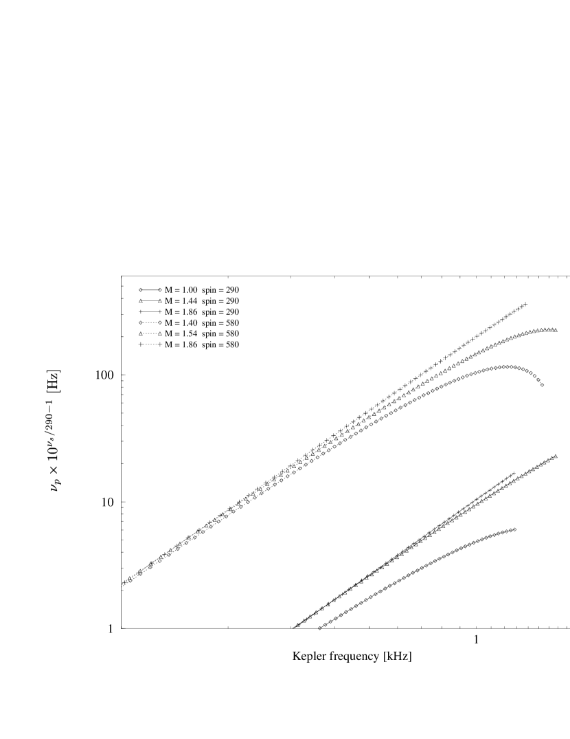
Figure 5: EOS C: Precession frequency versus orbital (Kepler) frequency for stars with spin frequency $\nu_{s}=290,580$ Hz. Each curve corresponds to a star with different mass. For clarity, the precession frequencies for stars rotating at a frequency of 580 Hz have been multiplied by a factor of 10.

In Figures 1 - 8 graphs of precession frequency versus Kepler (or orbital) frequency are plotted for a subset of the stars featured in tables 1 - 4. Each graph features a number of stars with two different angular frequencies, the more rapidly rotating stars (dotted lines) shifted upwards by a factor of 10 for clarity. The frequencies are plotted log-log to make it easy to discern departures from a power-law behaviour. Each curve corresponds to a different stellar model. Each point on the curve corresponds to a different radius at which the precession and orbital frequencies are evaluated.

The termination of each curve corresponds to the smallest radius (or highest orbital frequency) at which a particle can orbit the star. This limiting radius is either the surface of the star or the innermost stable circular orbit.

As an example of the use of these graphs, consider the power spectra displayed in Figure 3 of Strohmayer et. al. (1996) for the Atoll source 4U 1728-34, the neutron star of which rotates at $\nu_{s}\sim 360$ Hz. Broad peaks with centroids near 20, 26 and 35 Hz are clearly seen, which Stella and Vietri (1998a) propose to interpret as due to L-T precession. At the same time, the higher kHz QPOs, interpreted as the orbital frequency, are observed at $\sim 900$, 980 and 1100 Hz respectively. These data points do not lie along any of the curves on Figures 2, 4, 6 or 8.

Although the observational data for 4U1728-34 do not coincide with any of the theoretical curves, it can be seen that stellar models exist for which the observed QPOs are close to twice the theoretical precession frequencies. In table 5 we summarize the masses for each EOS which come closest to having precession frequencies which are one half the observed frequencies. We note that for EOS WFF3 and C, masses in the range $1.6M_{\odot}-1.86M_{\odot}$ provide the closest fits. For EOS L, a mass near $2.0M_{\odot}$ comes closest to producing precession frequencies near one half the observed values. It should be noted that for EOS L, the general relativistic effects produce a considerably smaller precession frequency than was predicted from the semi-Newtonian analysis done by Stella and Vietri (1998a).

Data from other atoll sources show a similar trend. For example, the source KS 1731-260 (Wijnands and van der Klis 1997) spinning at either $260$ or $520$ Hz, shows a broad feature centred about 27 Hz when the higher frequency kHz QPO is at 1200 Hz. Again, the predicted precession frequencies are close to half of what is observed, if the star is spinning with a frequency of 260 Hz. However, it the star is spinning at 520 Hz, then the theoretical precession frequencies are close to the observed QPO. In table 6 we summarize the masses which provide the closest fits to the data for KS 1731-260, assuming the neutron star is spinning with a frequency of 260 or 520 Hz.

The situation for the Z sources is a little different. These sources exhibit a somewhat more coherent peak in the $10-60$ Hz range, which is called the horizontal branch oscillation (HBO). For example, GX 17+2 (Wijnands et. al. 1997b) has a HBO peak at 60 Hz while the highest QPO is at 1000 Hz. This star is spinning at 290 Hz. The precession frequencies predicted for the softer EOS are of order 10 Hz for an orbital frequency of 1000 Hz, which a factor of $\sim 5-6$ too small to explain the observations. EOS L allows a precession of 20 Hz if the star is very heavy, $\sim 2.4M_{\odot}$, but this is still a factor of 3 too small. If the star is rotating at $580$ Hz, the predicted precession rate is still too low: EOS C predicts a precession rate of only 20 Hz for the $1.8M_{\odot}$ star. It seems unlikely that simple precession models explain the HBO peaks seen in the Z sources.

5.2 Accuracy of the post-Newtonian formula

We will now test the validity of a simplified post-Newtonian precession formula in the slow rotation limit. For simplicity we will consider a formula which ignores the centrifugal precession and the $O(j^{2})$ post-Newtonian correction to the quadrupole moment. The approximate formula is

$$\nu_{p}\simeq\nu_{LT}-\nu_{quad}(1+3\frac{GM}{rc^{2}}),$$ (51)

where the Lense-Thirring precession is

$$\nu_{LT}\simeq 13.2\;\frac{I}{\bar{M}}\;\nu_{s,2.5}\left(\nu_{K,3}\right)^{2}\ Hz$$ (52)

and the Newtonian quadrupole precession is

$$\nu_{quad}\simeq 3.5\;\Phi_{2,43}\;\left(\bar{M}\right)^{-5/3}\left(\nu_{K,3}\right)^{7/3}\ Hz.$$ (53)

In Eqs. (52) and (53) we have defined a number of scaled variables defined by: $\bar{M}=M/M_{\odot}$, $I_{45}=I/10^{45}$, $\Phi_{2,43}=\Phi_{2}/10^{43}$, $\nu_{s,2.5}=\nu_{s}/300$ and $\nu_{K,3}=\nu_{K}/10^{3}$.

In terms of the form factors $a(M,\hbox{EOS})$ given by Laarakkers and Poisson (1997), the Newtonian quadrupole precession is

$$\nu_{quad}\simeq 6.5\frac{a(M,\hbox{EOS})}{10}\left(\frac{I}{\bar{M}}\;\nu_{s,2.5}\right)^{2}\left(\bar{M}\right)^{-2/3}\left(\nu_{K,3}\right)^{7/3}\ Hz.$$ (54)

The post-Newtonian correction term is

$$3\frac{GM}{rc^{2}}\simeq 0.3\left(\bar{M}\right)^{2/3}\left(\nu_{K,3}\right)^{2/3}.$$ (55)

Consider, as an example, a moderately slowly rotating star such as the $M=1.0M_{\odot}$, $\nu_{s}=290$ Hz star described by EOS C. The surface of this star is the minimal radius allowed for both prograde and retrograde orbits. The formula (52) predicts a precession due to the Lense-Thirring effect of 20 Hz, given data from the first row of Table 3. From the definition given by Eq. (25), we find that $\nu_{K+}+\nu_{K-}=\omega/2\pi=20Hz$, as given by the slow rotation formula. The average of the prograde and retrograde precession frequencies, $\frac{1}{2}(\nu_{p+}+\nu_{p-})=19Hz$ also agrees with $\omega/2\pi$ within $0.5\%$. The precession due to oblateness Eq. (26) is $\nu_{oblate}=\frac{1}{2}(\nu_{p-}-\nu_{p+})=13Hz$. But the Newtonian quadrupole precession given by Eq. (53) is only 10 Hz. Inclusion of the post-Newtonian correction Eq. (55) increases this to 13.5 Hz corresponding to $4\%$ error. Clearly the post-Newtonian correction must be included close to the star. Finally we note that the centrifugal precession frequency is only $1\%$ of the quadrupole frequency (as given by the parameter $\zeta$ in the tables). Hence this frequency is small enough that it can be neglected. Since the parameter $\zeta$ reaches large values $\sim 10\%$ only when the quadrupole moment is small it seems likely that the centrifugal precession can always be ignored at this level of approximation.

In Figure 9 a comparison of the approximate post-Newtonian formula for the precession of prograde orbits with the exact results is made. Prograde precession frequencies for three EOS C stars with masses $1.0,1.4$ and $1.86M_{\odot}$, rotating with $\nu_{s}=290$ Hz are plotted versus orbital frequency. In each case the simplified post-Newtonian formula (51) is plotted as a dotted line, while the exact precession is plotted as a solid line. At orbital frequencies $\nu_{K}<1000$ Hz, the exact and approximate curves are indistinguishable. All of these models have $j<0.2$, and in this sense are slowly rotating. The precession frequency for stars with $j>0.2$ won’t be approximated very well by Eq. (51) and must be computed numerically.

5.3 Numerical accuracy

The numerical solutions which we find use a code (Stergioulas 1995) based on that of Cook et. al. (1994). The numerical grid is composed of 201 points in the radial direction and 101 points in the angular direction which is a finer grid than used by Cook et. al. This finer grid size was required to keep the errors in the numerically computed precession frequencies down to $1\%$. In the series expansions of the metric functions given by Eqs. (7) - (9), all terms up to and including $n=10$ were used. We checked that our numerical values of masses and radii agreed within $1\%$ of those found by Cook et. al. for EOS A and L.

To find the size of the absolute errors, we computed the precession for non-rotating stars with $M=1.4M_{\odot}$, the results of which are displayed in Figure 10. Theoretically, the precession of orbits is zero if the star is static. The numerically computed precession was less than $0.03$ Hz. The precession fell to less than $0.01$ at an orbital frequency of $1000$ Hz. These small but non-zero frequencies give a measure of the absolute numerical error inherent to our method.

A number of tests were done to check the validity of the frequencies found. Far from the star ($r/M>10$) one half the sum of the prograde and retrograde precession frequencies at constant radius must reduce to the standard expression for the Lense-Thirring precession,

$$\frac{1}{2}\left(\nu_{p+}+\nu_{p-}\right)=\frac{2J}{r^{3}}\left(1+O(j^{2})\right).$$ (56)

Similarly, the difference must reduce to the classical quadrupole precession,

$$\frac{1}{2}\left(\nu_{p+}-\nu_{p-}\right)=-\frac{3}{2}\nu_{K}\frac{\Phi_{2}}{Mr^{3}}\left(1+O(j^{2})\right).$$ (57)

The quantities $J$ and $\Phi_{2}$ can be computed independently of $\nu_{p\pm}$. Expressions (56) and (57) were satisfied to better than $1\%$ for large radii. The values of the precession frequencies in the strong field region near the ISCO were validated by noting that the expression on the left-hand-side of equation (56) should differ from the metric function $\omega/2\pi$ only at order $j^{3}$. (The computation of the precession frequencies depends on $\omega$ in a non-linear fashion through Eqs. (23) and (24), so this is a non-trivial comparison.) Hence the inequality

$$\frac{\pi\left(\nu_{p+}+\nu_{p-}\right)-\omega}{\omega}\leq O(j^{2})$$ (58)

must be satisfied. We found that the inequality (58) was satisfied for the models presented in this paper. When the value of the roation parameter took values $j\leq 0.2$, the left-hand-side of the inequality (58) was smaller than $j^{2}$, while it was larger than $j^{2}$ but of the same order of magnitude as $j^{2}$ when $j>0.2$. We conclude then that the precession frequencies computed are correct to within $1\%$.

6 Conclusion

We have computed the dependence of precession frequency on orbital frequency for a wide variety of neutron star masses, spins and equations of state. In doing so we have made a number of simplifying assumptions about the physics of the region close to the neutron star. The main assumptions used in this paper are:

1. Some physical mechanism exists to tilt the inner orbits of the accretion disk out of the star’s equatorial plane.

2. All forces on particles in the disk’s inner region besides gravity are negligible.

3. The perturbations causing the tilt create only an infinitesimal tilt angle.

We now consider the validity and ramifications of these assumptions.

It has long been thought that the combination of viscosity and gravito-magnetism always act to keep the inner ($r<100M$) region of an accretion disk co-planar with the star (Bardeen and Petterson 1975). However, recent calculations have shown that it is possible for warped precessing disk modes to exist in the inner disk region. Ipser (1996) applied perfect fluid perturbation theory to show that such modes are possible. The modes which he finds for the Kerr black hole metric are fairly low, $\leq 10Hz$. Adopting the formalism of Papaloizou and Pringle (1983), Marković and Lamb (1998) have included viscosity in the computation and have shown that a family of highly localised and weakly damped tilt modes exist close to the inner disk boundary which precess at a frequency very close to the local precession frequency. Alternatively it has been demonstrated that if the accretion disk matter is inhomogeneous, diamagnetic blobs can be lifted above the equatorial plane (where they will start precessing) through the resonant interaction with the star’s magnetic field (Vietri and Stella 1998).

Our assumption that gravity is the only force acting on particles in the inner region will not always be valid. Miller (1998) has shown that the interaction of radiation emitted close to the neutron star surface with the disk particles can have an important effect on the precession frequency, increasing it by a large factor. The effect is most pronounced for high luminosity sources (approaching the Eddington limit, such as Z-sources). However, it is unclear that the approach discussed by Miller (1998) is applicable to warped disks of high Thomson depth. In the framework of inhomogeneous accretion disks, the effects of radiation drag on individual diamagnetic blobs are probably negligible (Vietri and Stella 1998). In any case, the frequencies calculated in this paper should be treated as baseline frequencies for neutron stars which might be modified by the inclusion of other physics.

It seems reasonable to expect that the physical mechanisms explored so far will only produce a small tilt out of the equatorial plane. If, however, the tilt angle is large, the present results can nevertheless be used to estimate the precession frequency. To do so, we recall that the Lense-Thirring frequency is unaffected by the tilt angle, while the Newtonian quadrupole precession is multiplied by a factor of $\cos\beta$, where $\beta$ is the angle between the disk and the star’s equatorial plane. Inclusion of this factor in the approximate post-Newtonian formula (51) will provide a good estimate of the precession of orbits tilted by a large angle.

Finally, we note that the precession frequencies which we compute are a factor of $\sim 2$ smaller than the low-frequency ($\sim 20-35$ Hz) QPOs observed in the Atoll sources, that Stella and Vietri (1998a) interpreted in terms of precession frequency. In order for precession to explain these results, a physical or geometric mechanism to produce QPOs at twice the theoretical frequency must be developed. A possibility is that a modulation at twice the precession frequency is generated at the two points where the inclined orbit of diamagnetic blobs intersect the disk (Vietri and Stella 1998).

Figure 1: EOS A: Precession frequency versus orbital (Kepler) frequency for stars with spin frequency $\nu_{s}=290,580$ Hz. Each curve corresponds to a star with different mass. For clarity, the precession frequencies for stars rotating at a frequency of 580 Hz have been multiplied by a factor of 10.

Figure 2: EOS A: Precession frequency versus orbital (Kepler) frequency for stars with spin frequency $\nu_{s}=360,720$ Hz. Each curve corresponds to a star with different mass. For clarity, the precession frequencies for stars rotating at a frequency of 720 Hz have been multiplied by a factor of 10.

Figure 3: EOS WFF3: Precession frequency versus orbital (Kepler) frequency for stars with spin frequency $\nu_{s}=290,580$ Hz. Each curve corresponds to a star with different mass. For clarity, the precession frequencies for stars rotating at a frequency of 580 Hz have been multiplied by a factor of 10.

Figure 4: EOS WFF3: Precession frequency versus orbital (Kepler) frequency for stars with spin frequency $\nu_{s}=360,720$ Hz. Each curve corresponds to a star with different mass. For clarity, the precession frequencies for stars rotating at a frequency of 720 Hz have been multiplied by a factor of 10.

Figure 6: EOS C: Precession frequency versus orbital (Kepler) frequency for stars with spin frequency $\nu_{s}=360,720$ Hz. Each curve corresponds to a star with different mass. For clarity, the precession frequencies for stars rotating at a frequency of 720 Hz have been multiplied by a factor of 10.

Figure 7: EOS L: Precession frequency versus orbital (Kepler) frequency for stars with spin frequency $\nu_{s}=290,580$ Hz. Each curve corresponds to a star with different mass. For clarity, the precession frequencies for stars rotating at a frequency of 580 Hz have been multiplied by a factor of 10.

Figure 8: EOS L: Precession frequency versus orbital (Kepler) frequency for stars with spin frequency $\nu_{s}=360,720$ Hz. Each curve corresponds to a star with different mass. For clarity, the precession frequencies for stars rotating at a frequency of 720 Hz have been multiplied by a factor of 10.

Figure 9: Comparison of post-Newtonian and exact precession frequencies for EOS C and $\nu_{s}=290$ Hz

Figure 10: Precession frequencies for non-rotating stars with $M=1.4M_{\odot}$

Table 1: Precession frequencies, EOS A

							prograde				retrograde
$\bar{M}$	$\bar{M}_{B}$	$R$	$I/{\bar{M}}$	$\Phi_{2}$	$j$	$\zeta$	$r_{+}$	$\nu_{K}$	$\omega/2\pi$	$\nu_{p}$	$r_{-}$	$\nu_{K}$	$\omega/2\pi$	$\nu_{p}$
$\nu_{s}=290$ Hz
1.00	1.08	10.0	0.7	0.6	0.14	2	—	1.82	28.3	16.6	—	-1.85	28.3	38.1
1.05	1.15	10.0	0.7	0.6	0.13	2	—	1.88	30.9	19.2	10.1	-1.86	29.3	38.4
1.20	1.32	9.9	0.7	0.5	0.12	3	10.0	1.99	36.0	25.0	11.4	-1.67	24.4	29.9
1.41	1.59	9.6	0.7	0.4	0.11	5	11.8	1.69	26.3	21.8	13.2	-1.44	18.7	21.3
1.61	1.87	9.1	0.7	0.3	0.09	10	13.5	1.46	19.4	17.6	14.9	-1.28	14.5	15.5
1.66	1.95	8.4	0.6	0.2	0.08	15	14.1	1.41	16.3	15.3	15.4	-1.25	12.6	13.2
$\nu_{s}=360$ Hz
1.00	1.08	10.1	0.7	0.9	0.17	2	—	1.81	35.2	16.9	—	-1.85	35.2	49.9
1.03	1.12	10.0	0.7	0.9	0.17	2	—	1.85	37.0	18.7	10.2	-1.83	35.2	48.8
1.20	1.33	9.9	0.7	0.8	0.15	3	9.9	2.01	46.2	28.4	11.6	-1.62	28.7	36.3
1.41	1.60	9.6	0.7	0.7	0.13	5	11.7	1.71	34.1	26.7	13.4	-1.41	22.3	25.9
1.61	1.87	9.1	0.7	0.5	0.11	10	13.4	1.49	24.9	22.1	15.1	-1.26	17.3	18.8
1.66	1.95	8.5	0.6	0.3	0.10	15	13.9	1.43	21.3	19.6	15.5	-1.23	15.4	16.3
$\nu_{s}=580$ Hz
1.02	1.11	10.3	0.7	2.3	0.28	2	—	1.77	56.9	6.6	11.0	-1.66	46.8	74.3
1.25	1.39	10.0	0.7	2.1	0.24	3	10.1	2.01	77.7	29.1	12.8	-1.44	37.3	50.2
1.41	1.59	9.8	0.7	1.8	0.22	5	11.2	1.80	62.9	37.9	14.1	-1.32	31.8	39.3
1.46	1.66	9.7	0.7	1.7	0.21	6	11.7	1.73	58.2	38.6	14.6	-1.28	30.0	36.1
1.60	1.86	9.2	0.7	1.2	0.18	10	12.9	1.57	46.5	37.0	15.7	-1.20	25.6	29.0
1.67	1.95	8.7	0.7	0.9	0.17	14	13.5	1.50	39.4	34.0	16.1	-1.17	22.9	25.1
$\nu_{s}=720$ Hz
1.02	1.10	10.5	0.7	3.8	0.36	2	—	1.71	67.9	-12.0	11.6	-1.53	50.7	86.8
1.40	1.58	10.0	0.7	2.9	0.27	5	11.0	1.86	85.5	37.6	14.6	-1.26	36.7	47.1
1.58	1.82	9.4	0.7	2.1	0.24	9	12.4	1.65	65.7	45.7	15.9	-1.16	30.7	36.0
1.60	1.86	9.3	0.7	2.0	0.23	10	12.6	1.63	63.0	45.6	16.1	-1.15	29.9	34.7
1.67	1.95	8.8	0.7	1.4	0.21	14	13.2	1.55	53.7	43.6	16.5	-1.13	27.1	30.3

Table 2: Precession frequencies, EOS WFF3

							prograde				retrograde
$\bar{M}$	$\bar{M}_{B}$	$R$	$I/{\bar{M}}$	$\Phi_{2}$	$j$	$\zeta$	$r_{+}$	$\nu_{K}$	$\omega/2\pi$	$\nu_{p}$	$r_{-}$	$\nu_{K}$	$\omega/2\pi$	$\nu_{p}$
$\nu_{s}=290$ Hz
1.00	1.07	11.2	0.8	1.0	0.16	1	—	1.54	24.4	11.1	—	-1.56	24.4	35.5
1.16	1.26	11.2	0.8	1.0	0.15	2	—	1.66	30.1	16.2	11.3	-1.67	29.2	40.1
1.35	1.50	11.1	0.9	1.0	0.13	3	11.2	1.77	36.1	24.0	13.0	-1.46	23.5	29.2
1.41	1.57	11.0	0.9	0.9	0.13	4	11.7	1.71	33.7	24.2	13.5	-1.41	22.2	26.7
1.62	1.84	10.7	0.9	0.7	0.12	6	13.5	1.48	25.8	21.6	15.3	-1.24	17.7	19.9
1.85	2.16	9.8	0.8	0.5	0.10	13	15.5	1.28	18.1	16.5	17.2	-1.11	13.2	14.2
$\nu_{s}=360$ Hz
1.01	1.08	11.3	0.8	1.6	0.21	1	—	1.53	30.3	9.3	—	-1.56	30.3	47.1
1.12	1.22	11.2	0.8	1.5	0.19	2	—	1.62	35.5	15.1	11.3	-1.65	35.1	50.9
1.36	1.50	11.1	0.9	1.4	0.17	3	11.2	1.80	46.5	26.6	13.3	-1.41	27.4	35.2
1.41	1.57	11.1	0.9	1.4	0.16	3	11.6	1.73	43.4	27.3	13.8	-1.36	25.9	32.4
1.60	1.82	10.8	0.9	1.2	0.15	6	13.2	1.52	34.3	26.6	15.4	-1.22	21.4	24.8
1.84	2.16	9.9	0.9	0.7	0.12	12	15.3	1.30	23.6	21.0	17.4	-1.09	16.0	17.3
$\nu_{s}=580$ Hz
1.03	1.10	11.7	0.8	4.2	0.34	1	—	1.47	47.8	-10.1	11.7	-1.51	47.5	87.6
1.22	1.33	11.5	0.9	4.1	0.30	2	—	1.63	62.6	4.7	13.2	-1.37	41.1	63.8
1.43	1.60	11.3	0.9	3.7	0.27	4	11.4	1.78	77.6	24.6	14.9	-1.23	34.6	47.1
1.62	1.84	11.0	0.9	3.2	0.24	6	12.8	1.59	62.9	36.1	16.4	-1.13	29.6	36.7
1.70	1.95	10.8	0.9	2.8	0.23	7	13.4	1.52	56.6	38.0	17.1	-1.09	27.5	32.8
1.85	2.16	10.1	0.9	1.9	0.20	12	14.7	1.38	44.0	35.7	18.2	-1.03	23.3	26.1
$\nu_{s}=720$ Hz
1.01	1.08	12.2	0.9	7.1	0.45	1	—	1.37	54.5	-33.8	12.6	-1.36	49.2	99.9
1.40	1.55	11.6	0.9	6.2	0.35	3	—	1.73	93.4	1.5	15.4	-1.17	39.6	57.9
1.46	1.63	11.5	1.0	5.9	0.34	4	11.5	1.78	100.4	8.7	15.9	-1.14	37.8	53.3
1.61	1.82	11.2	1.0	5.2	0.31	6	12.5	1.65	86.6	32.5	17.0	-1.07	33.9	44.0
1.82	2.12	10.5	0.9	3.5	0.26	11	14.1	1.46	64.8	45.0	18.6	-1.00	28.2	32.9
1.86	2.17	10.2	0.9	3.0	0.25	12	14.4	1.43	60.3	44.7	18.8	-0.99	27.0	31.0

Table 3: Precession frequencies, EOS C

							prograde				retrograde
$\bar{M}$	$\bar{M}_{B}$	$R$	$I/{\bar{M}}$	$\Phi_{2}$	$j$	$\zeta$	$r_{+}$	$\nu_{K}$	$\omega/2\pi$	$\nu_{p}$	$r_{-}$	$\nu_{K}$	$\omega/2\pi$	$\nu_{p}$
$\nu_{s}=290$ Hz
1.00	1.07	12.7	0.9	1.6	0.19	1	—	1.28	20.1	6.0	—	-1.30	20.1	31.9
1.26	1.36	12.3	1.0	1.4	0.16	2	—	1.50	28.6	15.4	12.3	-1.52	28.2	38.7
1.40	1.53	12.0	1.0	1.3	0.15	3	—	1.63	34.0	21.2	13.5	-1.39	24.0	30.6
1.44	1.59	12.0	1.0	1.2	0.14	3	12.0	1.67	35.9	23.0	13.9	-1.36	22.9	28.6
1.60	1.79	11.6	1.0	1.0	0.13	5	13.3	1.50	28.8	22.3	15.3	-1.24	19.1	22.3
1.86	2.14	10.3	0.9	0.5	0.10	12	15.6	1.28	18.5	16.7	17.3	-1.10	13.4	14.5
$\nu_{s}=360$ Hz
1.01	1.08	12.8	1.0	2.5	0.24	1	—	1.27	24.9	3.0	—	-1.30	24.9	42.6
1.25	1.36	12.4	1.0	2.2	0.20	2	—	1.48	34.9	14.1	12.7	-1.46	32.6	47.4
1.40	1.54	12.1	1.0	1.9	0.18	3	—	1.62	42.3	22.4	13.9	-1.34	27.8	36.7
1.46	1.61	12.0	1.0	1.9	0.17	3	12.0	1.67	45.3	25.4	14.4	-1.30	26.2	33.6
1.59	1.77	11.7	1.0	1.6	0.16	5	13.0	1.54	38.4	26.6	15.4	-1.22	23.0	27.8
1.86	2.14	10.3	0.9	0.8	0.12	12	15.4	1.30	23.8	21.1	17.6	-1.08	16.1	17.5
$\nu_{s}=580$ Hz
1.03	1.10	13.6	1.0	7.4	0.41	1	—	1.18	37.8	-20.7	—	-1.22	37.8	79.1
1.14	1.22	13.3	1.0	6.9	0.38	1	—	1.29	45.0	-13.9	13.4	-1.31	43.7	82.4
1.40	1.53	12.6	1.0	5.5	0.31	3	—	1.53	64.5	8.3	15.1	-1.20	37.0	55.1
1.54	1.70	12.2	1.0	4.7	0.28	4	12.2	1.67	76.5	22.6	16.1	-1.14	33.1	44.9
1.79	2.03	11.2	1.0	3.0	0.23	8	14.1	1.45	54.1	37.4	17.9	-1.04	26.2	31.0
1.86	2.14	10.6	0.9	2.1	0.20	12	14.8	1.37	45.5	36.1	18.4	-1.02	23.6	26.7
$\nu_{s}=720$ Hz
1.09	1.16	14.5	1.1	12.9	0.53	1	—	1.10	44.8	-42.6	14.7	-1.14	43.6	98.1
1.41	1.53	13.0	1.1	9.3	0.40	3	—	1.46	76.8	-14.3	16.1	-1.10	39.8	63.2
1.60	1.78	12.3	1.1	7.3	0.34	5	12.5	1.65	96.1	14.0	17.4	-1.04	35.2	48.4
1.87	2.15	10.8	0.9	3.6	0.26	11	14.4	1.42	63.1	44.7	19.0	-0.97	27.5	31.9

Table 4: Precession frequencies, EOS L

							prograde				retrograde
$\bar{M}$	$\bar{M}_{B}$	$R$	$I/{\bar{M}}$	$\Phi_{2}$	$j$	$\zeta$	$r_{+}$	$\nu_{K}$	$\omega/2\pi$	$\nu_{p}$	$r_{-}$	$\nu_{K}$	$\omega/2\pi$	$\nu_{p}$
$\nu_{s}=290$ Hz
1.38	1.49	15.3	1.6	5.2	0.23	1	—	1.14	26.3	4.6	—	-1.17	26.3	43.4
1.49	1.61	15.3	1.6	5.3	0.22	1	—	1.18	29.0	7.4	15.4	-1.20	28.6	45.1
1.88	2.10	15.4	1.8	5.3	0.19	3	15.4	1.31	39.7	18.6	18.8	-0.99	21.7	29.0
2.19	2.49	15.3	1.9	4.9	0.18	5	17.8	1.13	31.3	21.1	21.5	-0.87	17.8	21.7
2.71	3.22	14.2	1.8	3.0	0.14	13	22.2	0.90	19.6	17.2	25.9	-0.73	12.4	13.6
$\nu_{s}=360$ Hz
1.29	1.39	15.5	1.5	8.0	0.31	1	—	1.09	29.4	-4.7	—	-1.12	29.4	55.2
1.45	1.57	15.5	1.6	8.3	0.29	1	—	1.14	34.5	0.1	15.8	-1.14	32.3	55.5
1.94	2.16	15.5	1.8	8.2	0.24	3	15.6	1.29	49.8	17.5	19.9	-0.93	24.0	32.9
2.01	2.25	15.5	1.8	8.1	0.24	4	16.2	1.25	47.3	19.8	20.5	-0.90	23.0	30.8
2.34	2.69	15.3	1.9	7.1	0.21	6	18.7	1.08	36.9	24.3	23.3	-0.80	18.9	22.9
2.71	3.22	14.3	1.9	4.8	0.18	13	21.8	0.93	26.1	21.9	26.4	-0.71	14.7	16.4
$\nu_{s}=580$ Hz
1.41	1.51	16.8	1.8	24.7	0.52	1	—	1.01	47.6	-46.5	18.5	-0.91	35.3	75.4
2.07	2.32	16.2	2.0	23.1	0.40	4	16.3	1.26	84.3	-10.5	23.3	-0.77	28.2	41.3
2.22	2.51	16.0	2.0	21.9	0.37	5	17.1	1.21	78.3	9.0	24.5	-0.73	26.5	36.6
2.40	2.75	15.8	2.0	19.9	0.35	7	18.2	1.14	70.4	24.5	25.9	-0.70	24.4	31.7
2.72	3.21	14.9	2.0	13.9	0.30	12	20.6	1.01	53.5	35.8	28.2	-0.65	20.5	24.1
$\nu_{s}=720$ Hz
1.55	1.67	18.9	2.1	47.4	0.68	2	—	0.90	54.5	-76.7	22.3	-0.73	32.3	69.6
2.00	2.21	17.3	2.1	42.2	0.54	3	—	1.15	93.3	-69.3	24.8	-0.69	30.4	49.4
2.17	2.43	16.9	2.1	39.4	0.51	4	17.0	1.22	106.7	-51.8	25.9	-0.67	28.9	43.4
2.40	2.74	16.4	2.1	34.8	0.46	6	18.0	1.17	98.6	-1.8	27.5	-0.64	26.7	36.6
2.73	3.20	15.4	2.1	24.6	0.39	11	19.8	1.06	78.8	38.4	29.7	-0.61	23.2	28.4

Table 5: Best fit neutron star models for 4U 1728-34

EOS	$\bar{M}$	$\nu_{s}$	$\nu_{K}$	$\nu_{p}$	$\nu_{K}$	$\nu_{p}$	$\nu_{K}$	$\nu_{p}$
WFF3	1.65	360	0.90	10.2	0.99	12.3	1.10	15.0
	1.78	360	0.90	10.4	0.99	12.5	1.10	15.3
	1.85	360	0.90	10.1	0.99	12.2	1.10	15.0
C	1.68	360	0.90	10.6	0.99	12.7	1.10	15.5
	1.80	360	0.90	10.8	0.99	13.0	1.10	15.9
	1.86	360	0.90	10.5	0.99	12.6	1.10	15.5
L	1.94	360	0.90	12.4	0.99	14.0	1.10	15.7
	2.03	360	0.90	13.7	0.99	15.7	1.10	18.0
	2.11	360	0.90	14.9	0.99	17.2	1.10	20.0

Table 6: Best fit neutron star models for KS 1731-260

EOS	$\bar{M}$	$\nu_{s}$	$\nu_{K}$	$\nu_{p}$
WFF3	1.61	260	1.20	13.2
	1.80	260	1.20	13.4
C	1.65	260	1.20	13.7
	1.80	260	1.20	14.0
	1.86	260	1.20	13.4
L	1.70	260	1.20	13.6
WFF3	1.72	520	1.20	23.8
	1.80	520	1.20	25.0
C	1.77	520	1.20	25.1
	1.86	520	1.20	25.5