Modeling the variability of the BL Lacertae object PKS 2155-304.

Abstract

The bright X-ray selected BL Lacertae object PKS 2155–304 has been the target of two intense multiwavelength campaigns, in November 1991 and in May 1994. Although the spectral energy distributions at both epochs were quite similar, the source exhibited two very distinct variability patterns that cannot be easily reconciled with homogeneous, one–zone jet models. During the first epoch the variability was almost achromatic in amplitude, with a time lag between X-rays and UV of $\approx 3$ h, while during the second epoch the variability amplitude increased as a function of wavelength, with the EUV flare peaking $\approx 1$ day after the X-ray flare. We model the source using a time-dependent inhomogeneous accelerating jet model. We reproduce the general characteristics of the different variability signatures by assuming that plasma disturbances with different physical properties propagate downstream in an underlying jet characterized by the same set of physical parameters at both epochs. A time delay of $\approx$ 1 day between the hardening of the UV spectral index and the UV flux, present at both epochs, is modeled with stochastic fluctuations in the particle acceleration manifested through small variations of the maximum energy of the injected electrons. We predict that similar time delays will be present in future observations, even in the absence of strong variability events. We stress the importance of observations at neighboring frequencies as a diagnostic tool for the structure of the quiescent jet in blazars, especially in the seemingly dull case when strong variability is absent.

1 INTRODUCTION

The X-ray selected BL Lacertae object (XBL) PKS 2155-304 is a nearby (z=0.116) bright blazar. The source has been monitored intensively twice in a frequency range from radio waves to X-rays. The first campaign took place during November 1991 (Edelson et al. (1995)). Observations were made at UV (Urry et al. (1993)), X-rays (Brinkmann et al. (1994)), and radio, infrared, and optical wavelengths (Courvoisier et al. (1995)). There was a flux increase by a factor of $\approx 2$ during the 30–day period of the campaign in the IR to X-ray frequency regime. Superposed on this slow variation were flares with an amplitude of $\approx 10\%$ and duration of $\approx 0.7$ days. The fractional amplitude of the variations appeared almost constant in the energy regime from IR to X-rays. The X-ray variations led the UV by $\approx 3$ h, while no delay down to a limit of $\approx 2$ h was found between the UV and the optical. These characteristics are difficult to reconcile with homogeneous synchrotron source models.

During the May 1994 campaign observations were made at X-ray (Kii et al. (1998)), extreme UV (Marshall et al. (1998)), UV (Pian et al. (1997)), and optical, IR, and radio wavelengths (Pesce et al. (1997)). The results are summarized by Urry et al. (1997). The ASCA observations recorded an X-ray flare on May 19. The flare was symmetric with a duration of $\approx 0.8$ days, and a relative amplitude of $\approx 2$ . The hard X-rays (2.2-8 KeV) led the soft X-rays (0.5-1 KeV) by $\approx 5000$ s (Kii et al. (1998)). EUVE recorded a flare that started on May 19 and lasted for $\approx 1.5$ days with a relative amplitude of $\approx 50\%$ (Marshall et al. (1998)). Cross–correlation analysis showed that the EUVE flare lagged the X-ray flare by $\approx 1$ day. Finally, IUE observations revealed a UV flare that peaked $\approx 2$ days after the X-ray flare with a relative amplitude of $\approx 35\%$ (Pian et al. (1997)). The IUE flare lasted for $\approx 2.5$ days. Although the variability behavior during these two campaigns was quite different, the spectral energy distributions (SEDs) at both epochs were very similar. This encourages us to identify the SED with the radiation produced by the underlying undisturbed jet and the variable emission with radiation from newly injected plasma components. The different variability signatures can then be interpreted simply as manifestations of different physical properties of the various plasma disturbances propagating along the jet.

2 THE MODEL

We use the accelerating inner jet model of Georganopoulos & Marscher (1998), upgraded to take into account the time evolution of the observed radiation due to a propagating disturbance in the plasma flow. The jet is characterized by the Lorentz factor $\Gamma_{\star}$ of the bulk motion of the injected plasma at the base of the jet, the distance $z_{\star}$ of the base of the jet from the stagnation point of the flow, the radius $r_{\star}$ of the base of the jet, and the exponent $\epsilon$ that describes how fast the jet opens and accelelerates ($r\propto z^{\epsilon}$, $\Gamma\propto z^{\epsilon}$). The injected plasma has an electron kinetic luminosity $\Lambda_{kin}$ and is characterized by a power law electron energy distribution (EED), $N(\gamma,z_{\star})=N_{\star}\gamma^{-s}$, $\gamma_{min}\leq\gamma\leq\gamma_{max}$. The comoving magnetic field, assumed predominantly tangled with a small component aligned to the jet axis, decays according to the relation $B\propto r^{-1}$. The electrons lose energy due to adiabatic and synchrotron losses, and the EED evolves as the plasma flows downstream, giving rise to a local non-power law synchrotron spectrum that evolves along the jet axis. This formulation does not include Compton losses, but in the case of PKS 2155–304 these are probably not the dominant energy loss mechanism (Vestrand et al. 1995).

The modeling of relativistically moving disturbances requires inclusion of light–travel time delays and light aberration, which have not been considered in previous calculations (Celotti, Maraschi, & Treves (1991)). If a disturbance travels with a speed $\beta c$ in a direction that forms an angle $\theta$ with the line of sight, the observed transverse velocity is

$$v=\frac{\beta c\sin\theta}{(1-\beta\cos\theta)(1+z)},$$

where z is the redshift of the source. This creates a combination of an apparent rotation and distortion of the disturbance front. We calculate the position of the disturbance as a function of time in the observer’s frame, taking into account relativistic time delays, and then perform the radiative transfer, taking into account the effect of light aberration (our treatment is similar to that of Gómez et al. 1994).

Modeling the steady-state, quiescent emission of a blazar requires a set of simultaneous multiwavelength data that correspond to the low state of the source. An extensive period of minor activity or the time before a significant event can be used as working definition of the low state of a jet. We construct (see Fig. 1) low state SEDs of PKS 2155-304 using multiwavelength data taken in 1991 November 14, during a period of 18 h (see Edelson et al. (1995)), and in 1994 May 18, during a period of $\approx 1$ day (see Urry et al. (1997)), when local flux minima, followed by a flare, were observed. The two SED appear quite similar, and, taking into account the problems of simultaneity and of definition of the quiescent state of the source, we assume that the undisturbed plasma flow at both epochs can be described adequately by one single set of physical parameters. We fit this composite two–epoch SED using the model parameters given in the caption of Figure 1. The solid curve in Figure 1 shows the steady–state model SED.

3 THE CAMPAIGN OF NOVEMBER 1991

We focus here on the short time scale ( $\approx 0.7$ days) variability, characterized by achromatic peak fractional amplitudes and a $\approx 3$ h time delay between X-ray and UV energies. We interpret the small time delays as an indication of near co–spatiality of the regions emitting the variable components at different frequencies. This can be achieved if the injected plasma component is characterized by a high magnetic field, so that the radiative loss time scale for the electrons emitting the X-ray photons is of the order of the observed time lag of $\approx 3$ h between the X-ray and the UV light curve. The fact that the doubling time scale inferred by the small amplitude ($\approx 10\%$) and the $\approx 0.7$ days flare duration, is longer than the observed 3 h time delay, implies that the duration of the flare is not due to radiative losses, but rather to the injection mechanism. This further implies that the size of the injected component is larger that the region that radiates at each frequency. As a result, the number of electrons that radiate at a given frequency band is a function of frequency in a manner similar to that of the underlying jet. This gives rise to a frequency independent fractional amplitude for the flare, as long as the spectral index of the variable component is similar to that of the underlying jet.

We assume that a “slug” of plasma characterized by a magnetic field $B_{inj}=1.2$ G was injected at the base of the jet. The injected electron kinetic luminosity increased linearly with time to reach a maximum amplitude of $\Lambda_{inj}=0.1\Lambda_{kin}$ after four hours (solid curve in Figure 2), and then declined linearly over four more hours. The shape and cutoff energies are assumed to have been the same as for the quiescent jet. The response of the jet is also shown in terms of the relative amplitude of the light curves at X-ray, UV, and optical energies. Figure 2 should be compared to Fig. 2 of Edelson et al. (1995). The time delays are in agreement with the observations, and the fractional amplitude of variability, although not precisely achromatic, does not vary significantly with frequency.

4 THE CAMPAIGN OF MAY 1994

The clear temporal separation between the peak flux at different frequencies translates into a spatial separation. Combining this with the assumption that a single plasma component propagating downstream was responsible for the observed variability, we again assume that a component of high energy electrons is injected at the base of the jet. As before, these electrons emitted synchrotron radiation at high frequencies (X-rays) and cooled as they propagated downstream, radiating at progressively lower frequencies. This can explain the time delays between the X-rays and the EUV and UV energies, but the longer time lags at the lower frequencies require the injected electron population to have beem more monoenergetic than in November 1991, i.e., $\gamma_{min}\rightarrow\gamma_{max}$. The relative amplitude of the flare was frequency dependent, with the higher frequencies characterised by a higher amplitude of variability (Urry et al. (1997)). Given the fact that the number of electrons that contribute to the underlying jet emission increases as the frequency decreases, the fixed number of electrons in the plasma component will give rise to a flare of higher relative amplitude at higher frequencies.

We therefore model the May 1994 flare with an injected EED confined by $2\times 10^{5}\leq\gamma\leq 7.5\times 10^{5}$, with $N(\gamma)\propto\gamma^{-s}$, $s=2.1$, and injected luminosity $\Lambda_{inj}=1.3\;\Lambda_{kin}$. We adopt for the duration of the injection event $t_{inj}=4$ h in the observer’s frame. In Figure 3 we plot the simulated light curves at different frequencies. In Figure 1 we plot the observed SED before and through the May 19 flare (the same data are plotted in Fig. 1 of Urry et al. 1997). The relative amplitudes and the time delays are in good agreement with the observations, with the exception of the amplitude of the UV flare, which had a relative amplitude of $35\%$, while the simulation gives an amplitude of $10\%$. An explanation for this discrepancy could be a mild re-acceleration of the electrons in the injected plasma component. Such a mild re-acceleration would be manifested mainly at lower frequencies, thereby increasing the flare amplitude relative to that at higher frequencies. An interesting feature is the $\approx 1$ hour time delay between the $3\times 10^{17}$ Hz and the $10^{17}$ Hz X-rays, as well as the smaller amplitude of the lower energy variation.

In Figure 4 we plot the X-ray spectral index versus X-ray flux diagram for the simulated flare. The amplitude of the X-ray spectral index variation ($\Delta\alpha\approx 0.3$) is slightly smaller than observed ($\Delta\alpha\approx 0.5$) We obtain the familiar clockwise loop that has been observed in X-ray variability studies of other sources (e.g. see Takahashi et al. (1996) for a similar curve in Mkn 421). Such a behavior is not universal and should be expected only for isolated flares that do not blend with any preceding or subsequent variability.

5 THE SPECTRAL INDEX – LUMINOSITY LAG

The results of cross–correlation analysis between the UV flux and spectral index, both for the November 91 flare (Urry et al. (1993)) and the May 94 flare (Pian et al. (1997)), show that the variation in the UV spectral index leads the change in intensity by $\approx 1$ day, in the sense that an increase (decrease) in intensity is preceded by a hardening (softening) of the spectral index. Given the very disparate variability behavior observed in the two campaigns, this similarity is not intuitively expected. Particularly puzzling at first look is the fact that the time delay persists in the May 94 campaign even after the central flare has been excluded from the cross–correlation analysis.

We propose that such a behavior is the response of the jet to small variations of the upper cutoff $\gamma_{max}$ of the injected EED. It is plausible that such stochastic fluctuations are always present, regardless of the existence or absence of major newly injected components that produce the large amplitude variability. Such variations are equivalent to the addition or subtraction of a small amplitude, nearly monoenergetic electron component that propagates downstream, affecting first the higher and then the lower frequencies. At neighboring frequencies this results in two low amplitude flares with the higher frequency flux peaking first. In Figure 5 we plot the cross–correlation function between the flux at 2000 Å and the 1400–2800 Å spectral index, when the upper cutoff $\gamma_{max}$ of the injected EED increases from $\gamma_{max}=7.5\times 10^{5}$ to $\gamma_{max}=7.6\times 10^{5}$ for eight hours, while the rate of injected particles is held constant. Although the variation amplitude is small ($\approx$ 1 %), the lag of $\approx 1$ day is the same as that observed (cf. Fig. 5 to Fig. 7 of Pian et al. 1997 and Fig. 9 of Urry et al. 1993).

Since this time lag is the response of the jet to stochastic variations of $\gamma_{max}$, we predict that the lag will be present in future observations of the source, particularly during intervals of mild activity when no major variability events occur, although the exact magnitude of the delay will depend on the nature of the variations. Similar considerations are relevant for all blazars. Observations at different frequencies will in principle produce time lags of different magnitudes. This “spectral fluctuation” technique can be used to constrain the geometry and physics of the quiescent jet, as well as provide information about the power spectrum of fluctuations in the density and energy distribution of the injected electrons. The method does not rely on the sporadic appearance of strong variability events, which in any case are related more to the newly injected components and less to the underlying jet flow. Mild variability of the order of a few percent is sufficient for the cross–correlation analysis.

This research was supported in part by NASA Astrophysical Theory Program grant NAG5-3839.

Figure 1: The spectral energy distribution (SED) of PKS 2155-304 for 14 November 1991 (triangles; Edelson et al. 1995), and 19 May 1994 (diamonds; Urry et al. 1997). The data of 16.5 May 1994 (asterisks) were selected by Urry et al. (1997) to represent the pre-flare SED. The filled symbols represent the observed time evolution of the SED during the 19 May 1994 flare. The solid curve represents the steady–state model SED. The broken curves represent the time evolution of the simulated flux during the May 94 flare. The flare starts at time t=0 in the observer’s frame, which corresponds to $\approx 19.1$ May. The values of the steady–state model parameters are: $r_{\star}=10^{15}$ cm, $z_{\star}=1.3\;10^{15}$ cm, $\Gamma_{\star}=1.5$, $\epsilon=0.3$, $B_{\star}=0.1$ G, $\Lambda_{kin}=10^{46}$ erg/s, $\gamma_{max}=7.5\;10^{5}$, $s=1.7$, and $\theta=14^{\circ}$.

Figure 2: Simulated light curves for the November 91 campaign.

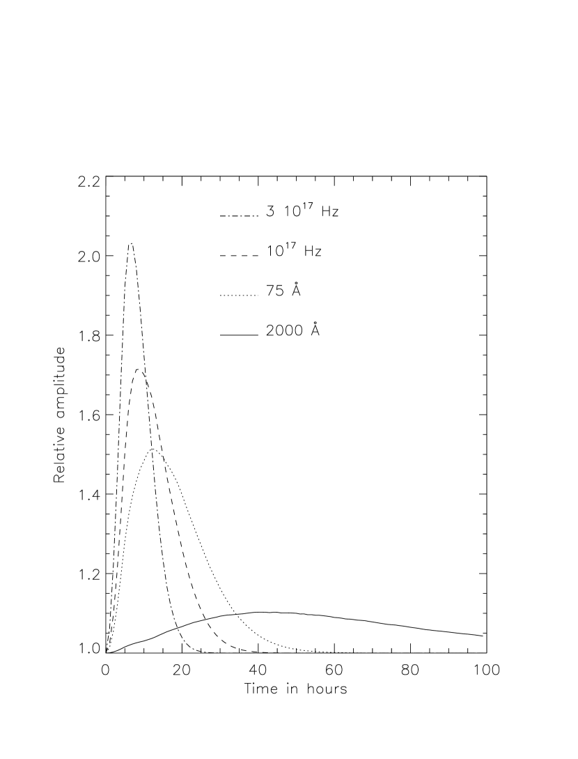
Figure 3: Simulated light curves for the May 94 campaign.

Figure 4: Model X-ray spectral index vs X-ray flux for the May 1994 flare. The integers following the clockwise loop indicate time in hours.

Figure 5: Cross–correlation function between the model flux at 2000 Å and the 1400–2800 Å spectral index. The spectrum flattens (steepens) $\approx 1$ day before the flux increases (decreases).

References

- Brinkmann et al. (1994) Brinkmann, W., et al. 1994, A&A, 288, 433
- Celotti, Maraschi, & Treves (1991) Celotti, A., Maraschi, L., & Treves, A. 1991, ApJ, 377, 403
- Courvoisier et al. (1995) Courvoisier, T. J. - L., et al. 1995, ApJ, 438, 108
- Edelson et al. (1995) Edelson, R. et al. 1995, ApJ, 438, 120
- Georganopoulos & Marscher (1998) Georganopoulos, M., & Marscher, A. P. 1998, ApJ, submitted
- Gómez et al. (1994) Gómez, J. L., Alberdi, A., Marcaide, J. M., Marscher, A. P., & Travis, J. P. 1994, A&A, 292, 33
- Kii et al. (1998) Kii, Y., et al. 1998, in preparation
- Marshall et al. (1998) Marshall, H. L., et al. 1998, in preparation
- Pesce et al. (1997) Pesce, J. E. 1997, ApJ, 486, 770
- Pian et al. (1997) Pian, E. 1997, ApJ, 486, 784
- Takahashi et al. (1996) Takahashi, T. et al. 1996, ApJ, 470, L89
- Urry et al. (1993) Urry, C. M., et al. 1993, ApJ, 411, 614
- Urry et al. (1997) Urry, C. M., et al. 1997, ApJ, 486, 799
- Vestrand, Stacy, & Sreekumar (1995) Vestrand, W. T., Stacy, J. G., & Sreekumar, P. 1995, ApJ, 454, L93