HIGH OBSERVED BRIGHTNESSES IN RADIO JETS

Abstract

We study the variability properties at radio frequencies of the jets thought to be typical of Active Galactic Nuclei, i.e. bulk Lorentz factor $\Gamma\approx$10, and incoherent synchrotron emission. We assume that the radiating electrons are accelerated at shocks within the jet, and that these shocks have a suitable (conical) geometry. In our framework, we can reproduce the variability pattern of Intra Day Variables (20% in less than 1 day) as long as the observed brightness temperature is $T_{B}<3~{}10^{17}$ K. The only stringent condition is an injection timescale of the perturbation shorter than the variability timescale; the geometric condition on the viewing direction is not especially severe, and agrees with the observed occurrence of the phenomenon. For higher values of $T_{B}$ coherent processes are probably necessary.

1 INTRODUCTION

One of the defining features of Active Galactic Nuclei (AGN’s) is flux variability over most of the electromagnetic spectrum, with observed timescales which range from minutes up to several years (Ulrich, Maraschi & Urry (1997)); the information content of the variations makes them a fundamental clue for the understanding of AGN’s. In a previous paper (Salvati, Spada & Pacini (1998), hereafter Paper I) we have considered the extremely fast variations (duration of about 20 minutes) observed in the TeV range from Mkn 421 (Gaidos et al. (1996)). These flares imply an extremely compact emitting region and a very high photon-photon opacity, unless the source is moving with bulk Lorentz factor $\Gamma\approx 100$ (see also Celotti, Fabian & Rees (1998)). We have shown that extreme jet parameters are not needed, however, if the photon distribution is anisotropic in the comoving frame; such a distribution is a natural consequence of conical shocks, with opening angle $\approx 1/\Gamma$.

At the opposite end of the e.m. spectrum, similar problems are presented by fast radio variations. Although radio emission occurs at much larger scales than TeV emission ($10^{19}-10^{20}$ cm versus $10^{16}-10^{17}$ cm), variability up to a level $\approx$ 20% has been observed in various sources with timescales shorter than a day, the so called Intra Day Variability (IDV) (Wagner & Witzel (1995), hereafter WW). The observations imply brightness temperatures up to $10^{18}-10^{19}$ K, well above the Compton limit $10^{12}$ K (Kellermann & Pauliny-Toth (1968)). Because of the relativistic motion of the source the intrinsic $T^{c}_{B}$ is $\Gamma^{3}$ lower than the brightness temperature derived from the light curves (WW; Rees (1966)). Again, bulk Lorentz factors $\Gamma\approx 100$ would be required to cure the problem (see also Begelman, Rees & Sikora (1994)). VLBI observations indicate $\Gamma$ $\approx$ 10 only (Vermeulen & Cohen (1994); Ghisellini et al. (1993)), so the intrinsic $T^{c}_{B}$ remains well above $10^{12}$ K, even after the beaming effects have been corrected for.

Our purpose in this paper is to show that the model developed earlier to interpret the high energy variability may be relevant to the radio variability as well, with some appropriate modifications. We shall show that in this way one can account for $T_{B}$ up to several times $10^{17}$ K. Higher values of $T_{B}$ wich have been claimed would however defy our interpretation. This is especially true for PKS0405–385 (Kedziora-Chudczer et al. (1997)), which varied on timescales of minutes with $T_{B}\sim 10^{21}$ K. Barring a relativistic jet with $\Gamma\sim 10^{3}$, here one is compelled to accept intrinsically high brightnesses, due perhaps to coherent processes.

2 DESCRIPTION OF THE MODEL

Light travel time effects are important in the modelling of variability since they change the observed time with respect to the coordinate time by the factor $1-\beta{\rm cos}\theta$, with $\beta$ the velocity of the source in units of $c$, and $\theta$ the angle between the velocity vector and the line of sight. If the relevant source velocity is a physical velocity, one recovers the well known “shortening” factor $\sim 1/\Gamma^{2}$. In our scheme, the perturbation is modelled as a slab of extra electrons superposed on the steady jet, and flowing down the jet with the same bulk Lorentz factor $\Gamma$; the extra electrons radiate only after having passed through an oblique (conical) shock, where they are accelerated to relativistic energies in the comoving frame; that is, instead of radiating simultaneously, they radiate in succession according to their distance from the shock apex (see Fig. 1 for details). The relevant source velocity, then, is the phase velocity of the intersection point between the slab and the shock; calling $\alpha$ the incidence angle, we rewrite the “shortening” factor as $1-\beta{\rm cos}(\theta-\alpha)/{\rm cos}\alpha$, with $\beta$ the physical velocity corresponding to $\Gamma$, and $\beta/{\rm cos}\alpha$ the phase velocity. The viewing angle is measured with respect to the phase velocity, i.e. from a generatrix of the cone, and is $(\theta-\alpha)$ if we measure $\theta$ with respect to the physical velocity. As already pointed out in Paper I, arbitrarily fast variations can be observed when ${\rm cos}\alpha=\beta$ and $\theta=\alpha$.

Oblique shocks with $\alpha\approx 1/\Gamma$ are indeed expected in relativistic jets. If the external pressure drops suddenly, the jet decollimates and recollimates through a series of alternating conical shocks with this kind of aperture (Bowman 1994; Gómez et al. 1997). Furthermore, radio jets are observed to bend away from their initial direction already at the parsec scale; these deviations are probably amplified by projection effects, and are due to grazing collisions between the jet and the irregularities of the ambient medium. In this context, one should note that the transverse pressure exerted by the jet on the ambient medium is made up of two parts, the comoving pressure and the ram pressure, of which only the latter increases strongly with $\Gamma$ for incidence angles larger than $1/\Gamma$. It is then plausible that the external medium will give way until angles of this magnitude are reached. Of course, the shock will not be conical in this case; however, the variability is dominated by that part of the perturbation which is closest to the line of sight. All other parts add up on much longer timescales and contribute to the “steady” emission of the jet, so that a precise treatment of their timing is unnecessary.

The condition that the viewing angle $(\theta-\alpha)$ be small is not very restrictive: the sources which we study are selected a priori to belong to the blazar class, and the line of sight is selected a priori to be aligned with the jet at angles $\theta\leq 1/\Gamma$ (Urry & Padovani 1995); within the “blazing” cone, the major part of the solid angle resides close the cone surface, $\theta\approx 1/\Gamma$, which is our requirement for fast variations.

The length of the injection time determines the thickness of the slab representing the perturbation, and constitutes a firm lower limit for the variability timescale. It is tenable that the injection time is determined by the central engine, the black hole, and that the flow is modulated with the hole crossing time even at distances much larger than the hole radius. Here we follow an analogy with the models invoked for gamma-ray bursts (Rees & Mészáros 1992, 1994): the hyperrelativistic blast wave radiates the burst at a fraction of a light year, with a “global” timescale determined by the distance times $1/\Gamma^{2}$; on a finer scale, however, the light curve is modulated with a time typical of the central engine, a neutron star, whose dimensions have remained imprinted in the flow notwithstanding the enormous expansion. In the case of AGN’s, this minimum modulation time could be of a few minutes, compatible with the fastest variations observed.

Fast variability at radio frequencies, in comparison with gamma-ray frequencies, has additional features which must be considered. The lifetime of the radio emitting electrons is much longer than the gamma-ray one: in the former case, then, at any given coordinate time radiation is emitted not only by the electrons which have just been shocked, but also by older electrons shocked previously, which (see Fig. 1) travel at different distances from the jet axis. Given the very long lifetime of the relevant electrons, the emission region can cover the entire cross section of the jet, even if one includes the decline of the emissivity due to the lateral expansion of the flow. The observed light curve is severely smoothed for a generic line of sight. In the following, we show that in a region of the parameter space fast variability is nonetheless possible, and that this region is ample enough to account for the observed statistics.

A final caveat is related with the duty cycle of fast variability at radio frequencies. Intra Day Variables exhibit long periods of continuous activity, with many outbursts superposed at any given time, while at gamma-ray frequencies the outbursts seem isolated (observational constraints might play a role here). Our model is better suited to account for isolated outbursts, since the unfavored parts of each slab emit on longer timescales, and superpose with other slabs to raise the “steady” level of the source. The fast varying emission is diluted to a small fraction of the total when many slabs are seen simultaneously. This is in qualitative agreement with the data, since the gamma-ray flux varies by large factors, whereas IDV is of the order of a few percent only. At any rate, a quantitative analysis requires a more realistic description than that of Paper I: here we include properly the dynamics of the flow across the shock, and the angular distribution of the radiation after the shock.

3 THE FORMALISM OF THE MODEL

The flow takes place within a funnel with rigid walls. The walls have an opening angle $\psi$ with respect to the $z$ axis, the symmetry axis of the system, and a relativistic beam of cold plasma impinges on them at an angle $\eta$ (Fig. 1). Before the shock the bulk velocity is $v_{1}\approx c$ and the Lorentz factor $\Gamma_{1}>>1$. Since the bulk velocity after the shock, $v_{2}$, must be parallel to the wall, the Rankine-Hugoniot conditions (see, e.g., Kennel & Coroniti (1984)) establish the Lorentz factor downstream, $\Gamma_{2}$, and the position of the shock with respect to the initial direction of the beam – i.e. the angle $\alpha$ of Fig. 1. In the frame $S^{*}$ where the shock is perpendicular the Lorentz factor upstream is $\Gamma_{1}^{*}=\sqrt{\Gamma_{1}^{2}\sin^{2}\alpha+\cos^{2}\alpha}$, with $\Gamma_{1}^{*}\approx\Gamma_{1}$ for angles $\alpha$ near $\pi/2$ and $\Gamma_{1}^{*}\leq\sqrt{2}$ when $\alpha\leq 1/\Gamma_{1}$. The shock is not relativistic in general, so the exact solution of the Rankine-Hugoniot conditions is complicated, and we approximate it as follows:

$$v_{2}^{*}=\frac{c}{3}\sqrt{1-\frac{41}{25}\frac{1}{(\Gamma_{1}^{*})^{2}}+\frac{16}{25}\frac{1}{(\Gamma_{1}^{*})^{4}}}$$ (1)

This expression reproduces the two limiting solutions: $v_{2}^{*}=v_{1}^{*}/3\approx c/3$ for a relativistic shock ($\Gamma_{1}^{*}>>1$); and $v_{2}^{*}=v_{1}^{*}/5$ in the opposite case ($\Gamma_{1}^{*}\leq\sqrt{2}$), under the assumption that the electrons become relativistically hot even if the protons do not. In the laboratory frame, finally, the Lorentz factor downstream is:

$$\Gamma_{2}=\frac{1}{\sqrt{1-\left(\frac{v_{1}}{c}\right)^{2}\cos^{2}\alpha+\left(\frac{v_{2}^{*}}{c}\right)^{2}(1-\left(\frac{v_{1}}{c}\right)^{2}\cos^{2}\alpha)}}$$ (2)

where $\alpha$ is determined by making $v_{2}$ parallel to the wall:

$$\tan{\epsilon}=\frac{v_{2}^{*}}{v_{1}\cos{\alpha}}\sqrt{(1-\left(\frac{v_{1}}{c}\right)^{2}\cos^{2}\alpha)}$$ (3)

and $\epsilon=\alpha-\eta$ is the angle between the shock and the wall.

After the shock the electrons radiate effectively for a distance $\Delta s\leq z$. If $t$ is the coordinate time, the plasma meets the shock in $z=v_{1}t\cos(\psi-\epsilon)/\cos\alpha$, and the emission region is a ring in the $x-y$ plane with internal radius $r=v_{1}~{}t~{}\sin(\psi-\epsilon)/\cos\alpha$. The non–zero particle lifetime gives the width of the ring : $\Delta r=\Delta s~{}(\sin\psi-\cos\psi~{}\tan(\psi-\epsilon))$ (Fig. 1). The relation between the coordinate time $t$ and the observed time $t_{o}$ ( the time at which a given wavefront reaches the observer) yields the infinitesimal surface element of the ring in $t$ which contributes to the radiation observed in $t_{o}$:

$$\Delta A(t_{o},t)=\Delta y(t_{o},t)~{}|\frac{dx}{dt_{o}}|_{t}$$ (4)

$$\Delta y(t_{o},t)=\sqrt{(r+\Delta r)^{2}-x^{2}}-\sqrt{r^{2}-x^{2}},~{}~{}~{}x=-\frac{c}{\sin\theta}[t_{o}-t(1-\frac{v_{1}}{c}\frac{\cos(\psi-\epsilon)}{\cos\alpha}\cos\theta)]$$ (5)

The integral of Eq. 4 with respect to $t$ – weighted with the radiation pattern $P$ of Eq. 7 – gives the area $A_{w}(t_{o})$ of the source region that generates the flux in $t_{o}$, $F(t_{o})$; this region is still ring–shaped, but lies in a plane inclined at an angle $\xi$ with respect to $z$, $\tan\xi=[(\cos\alpha/\cos(\psi-\epsilon)-\frac{v_{1}}{c}\cos\theta)/(\frac{v_{1}}{c}\sin\theta)]$. The flux in $t_{o}$ is proportional to $A_{w}(t_{o})$, and we can describe the light curves at different frequencies by an appropriate choice of $\Delta s$.

The high frequencies are radiated by energetic electrons, which cool very quickly so that $\Delta r<<r$; then the model predicts sharp flares with timescales $<<\Delta t_{z}$ for $\alpha\approx 1/\Gamma_{1}$ and for lines of sight close to a generatrix of the shock, $\theta\approx\theta_{p}=\psi-\epsilon$ (Paper I). At low frequencies the lifetime of the particles increases and $\Delta r$ increases too, until it becomes comparable to $r$. The light curve is smoothed, and the shortest variability timescale approaches the crossing time $\Delta t_{z}$. In order to observe sharp temporal features the viewing angle $\theta$ must be close to $\theta_{p}$, and at the same time be such that $\xi(\theta)$ is close to $\psi$. In this geometry $\vec{\Delta s}$ is parallel to the surface $A(t_{o})$ that contributes to the radiation at a given $t_{o}$: the photons emitted by the electrons during their lifetime reach the observer at the same instant, and the light curve is independent of $\Delta s$. The angle $\theta$ for which this occurs is:

$$\cos{\theta_{\xi}}=\frac{\cos{\alpha}\pm|\tan{\psi}|\sqrt{\left(\frac{v_{1}}{c}\right)^{2}\cos^{2}{(\psi-\epsilon)}(\tan^{2}{\psi}+1)-\cos^{2}{\alpha}}}{\frac{v_{1}}{c}\cos{(\psi-\epsilon)}(1+\tan^{2}{\psi})}$$ (6)

Fig. 2 shows the theoretical light curves for different viewing angles around $\theta_{\xi}$. If we assume $\Gamma_{1}=15$, $\alpha=1/\Gamma_{1}$ and $\psi=0.1$, then $\theta_{\xi}\approx 0.04$, $\theta_{p}\approx 0.08$, and $\Gamma_{2}\approx 10$. If $r_{0}$ is the initial jet radius, the light curves are computed assuming that $\Delta s=10~{}r_{0}$: over this distance the jet radius doubles, and the emissivity drops by a factor of several. The variability is about 25% on a time scale $\approx 0.1\Delta t_{z}$, if $\theta$ is between 0.04 and 0.06.

The light curves in Fig. 2 are computed with a realistic angular distribution of the radiation. In the frame comoving with the plasma the magnetic field upstream is assumed isotropic, downstream the magnetic field component parallel to the shock $B_{//}$ dominates the normal one $B_{\perp}$, even if $\Gamma_{1}^{*}\sim 1$. Including only $B_{//}$ and transforming back to the laboratory frame, we get

$$\frac{dP(\chi,\phi)}{d\Omega}\propto\left[1+\left(\frac{\sin{\epsilon_{c}}(\cos{\chi}-\frac{v_{2}}{c})}{1-\frac{v_{2}}{c}\cos{\chi}}+\frac{\cos{\epsilon_{c}}\sin{\chi}}{\Gamma_{2}(1-\frac{v_{2}}{c}\cos{\chi})\sqrt{1+\tan^{2}{\phi}}}\right)^{2}\right]\frac{\delta^{3}}{\Gamma_{2}}$$ (7)

where $P$ is the power emitted in a unit solid angle in the direction defined by $\chi$ and $\phi$, $\delta=[\Gamma_{2}~{}(1-v_{2}/c~{}\cos{\chi})]$ is the Doppler factor, $\epsilon_{c}=\tan(\alpha-\eta)/\Gamma_{2}$ is the angle between the shock and the wall in the comoving frame after the shock, and

$$\cos{\chi}=\cos{\theta}\cos{\psi}(1+\frac{x}{r}\tan{\theta}\tan{\psi})$$ (8)

$$\tan{\phi}=\frac{\tan{\theta}\sqrt{1-(x/r)^{2}}}{\sin{\psi}}$$ (9)

If $x^{\prime}$,$y^{\prime}$,$z^{\prime}$ are cartesian coordinates with $z^{\prime}$ along $v_{2}$ (parallel to the wall), the $z^{\prime}x^{\prime}$, and $x^{\prime}y^{\prime}$ sections of the radiation pattern for $\Gamma_{1}$=15 and $\alpha=1/\Gamma_{1}$ are shown in Fig. 3. If the opposite walls of the funnel diverge by an angle $\geq$ the width of the radiation pattern, the long–lasting tail of a flare due to the ‘unfavored’ side of the funnel is much suppressed; this is important when modeling light curves which, as the radio ones, show repeated flares with a high duty cycle.

4 COMPARISON WITH THE DATA AND DISCUSSION

Fig. 4 shows the comparison of a theoretical light curve with the observations of S5 0716+714 (Wagner et al. (1996)). This source is classified as a BL–Lac object, with a bright (S${}_{5~{}GHz}>1$ Jy) and flat radio emission ($S_{\nu}\propto\nu^{\alpha}$ with $\alpha=0.42$ between 1.5 and 5 GHz, Ghisellini et al. (1997)), and a significant optical polarization. The optical spectrum is completely featureless and the redshift determination is difficult. The absence of any host galaxy rules out redshifts $z<0.25$ and it is generally assumed $z>0.3$.

The light curve in Fig. 4 represents the VLA observations of February 1990. The source was observed at $\lambda=6$ cm every two hours, with a regular sampling (except for weekly maintenance gaps). Normalized to the average brightness, the light curve shows intraday variability, in particular in the first part of the campaign.

The theoretical light curve in the lower panel was obtained by convolving many curves like those of Fig. 2, with random initial times and amplitudes. The time separation between successive microflares has a flat distribution between 0.025 and 0.075 $\times\Delta t_{z}$, the amplitude has a flat top distribution of relative width 20%. The parameters of the elementary curves are equal to the those of Fig. 2, with $\theta=0.04$. The choice of the intrinsic time $r_{0}/(c\Gamma_{1})$ sets the physical size of the source and the variability timescale; here we have taken $r_{0}/(c\Gamma_{1})$=13 days. Since similar results are obtained with larger $\theta$’s up to 0.06, the visibility fraction is $(0.06^{2}-0.04^{2})\times\Gamma_{2}^{2}\approx$0.24, in good agreement with the occurrence of Intra Day Variability in the Effelsberg catalog. Indeed, our results are valid when the line of sight is at a small angle with respect to the shock surface; since the line of sight must be a priori within $1/\Gamma_{2}$ of the same surface, in order that the source shows blazar features, the visibility fraction is substantial. The model by Qian et al. (1991) is similar to ours in requiring an injection timescale shorter than the variability timescale; on top of this, the line of sight must be at a small angle with respect to the symmetry axis, instead of the shock surface, and the visibility fraction is diminished with respect to ours by a factor of order $1/\Gamma_{2}$.

A final parameter to be chosen is the average flux, to which the curves are normalized. If the comoving brightness temperature is $T^{c}_{B}$, $q_{0}=1/2$ and $H_{0}=70\rm~{}km~{}s^{-1}~{}Mpc^{-1}$, the flux emerging from the base of the cone in Fig. 1 can be written as

$$F_{\nu}=\frac{2\nu^{2}(1+z)^{3}k_{B}\Gamma_{2}T^{c}_{B}3\pi[c\Gamma_{1}~{}13~{}{\rm days}/(1+z)]^{2}}{(9~{}{\rm Gpc}\times(1+z-\sqrt{1+z}))^{2}}$$ (10)

The maximum value for $T^{c}_{B}$ is 10¹² K, of course. At relatively low redshifts, appropriate to objects like S5 0716+714, we obtain fluxes of the order of those observed in the S5 catalog, i.e. about a Jansky.

The particular source in question, S5 0716+714, was chosen as a paradigm of IDV at low redshifts because of the extensive data base, and from this point of view the performance of the model is comforting. However, S5 0716+714 is also the only firm example of correlated optical and radio IDV (WW). Most models have the high frequency emission coming from the inner jet, at distances of about 10¹⁶–10¹⁷ cm, and the radio emission from further out, at distances of about 10¹⁹–10²⁰ cm. If the correlation is accounted for by making cospatial the optical and the radio, then the canonical scheme must be abandoned: placing the radio source in the inner jet would imply extreme brightness temperatures and coherent processes (see below). Moving the high frequency source further out would be compatible with the scheme proposed here, but would be difficult to reconcile with models involving inverse Compton, because of the low density of targets; one could perhaps resort to models involving proton induced cascades (Mannheim 1993).

At redshifts of order 1 and higher, appropriate to quasar IDV’s, the fluxes predicted by Eq. 10 are too low. We can obtain reasonable fluxes by taking higher values for $r_{0}/(c\Gamma_{1})$, at the expense of longer variability timescales. These limitations amount to an upper bound on the apparent brightness temperature of several times 10¹⁷ K (with the same definitions of WW). We conclude that, while a non–negligible fraction of IDV’s can in principle be accounted for by our model, the extreme events, and especially the 10²¹ K flare observed in PKS0405–385, may involved alternative scenarios as coherence.

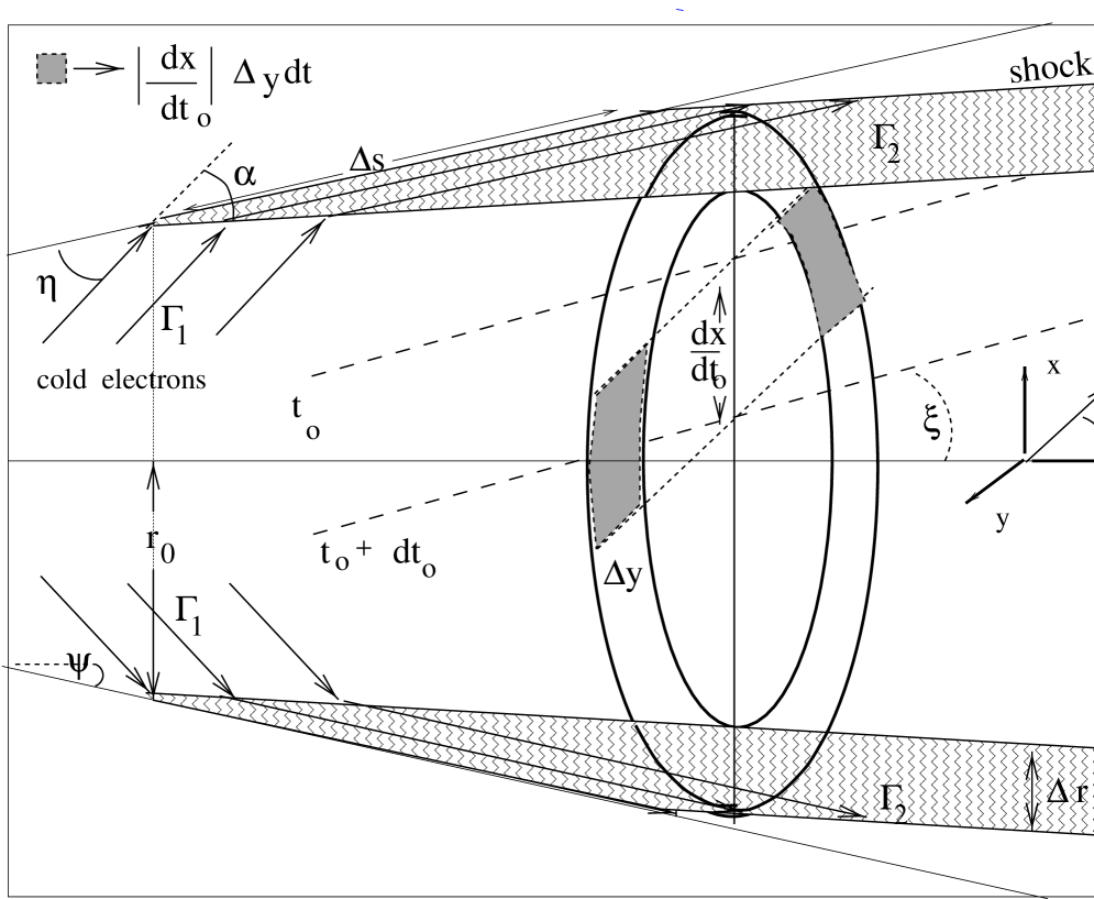
Figure 1: The source geometry. A beam of cold electrons ($\Gamma_{1}$) impinges on the jet walls at an angle $\eta$ . A shock is formed at an angle $\alpha$ with the initial velocity of the particles, and the electrons became relativistic in the comoving frame (dashed part). They move along the jet walls ($\Gamma_{2}$) and radiate for a distance $\Delta s$. The viewing angle is $\theta$. The ring in the figure is the emission region at the coordinate time $t$. Only the filled part of this ring ($\Delta A=\Delta y|dx/dt_{o}|_{t}$) contributes to the flux $F(t_{o})$. The two dashed lines indicate the positions of the planes (normal to the page, and inclined by $\xi$ with respect to $z$), from which the photons emitted at different $t$’s arrive together to the observer between $t_{o}$ and $t_{o}+dt_{o}$.

Figure 2: The theoretical light curves for different viewing angles around $\theta_{\xi}=0.042$, with $\Gamma_{1}=15$, $\alpha=1/\Gamma_{1}$, $\psi=0.1$ and $\Delta s=10~{}r_{0}$. The time is normalized to the crossing time $\Delta t_{z}$ and the flux $F(t_{o})$ to its average value. If $\theta$ is between 0.04 and 0.06, the variability is about $25\%$ on a timescale of $\approx 0.1\Delta t_{z}$.

Figure 3: The radiation pattern for $\Gamma_{1}=15$ and $\alpha=1/\Gamma_{1}$. If $x^{\prime}$,$y^{\prime}$,$z^{\prime}$ are cartesian coordinates with $z^{\prime}$ along $v_{2}$, the upper panel shows the section $x^{\prime}z^{\prime}$, and the bottom one the section $x^{\prime}y^{\prime}$.

Figure 4: The observed (top panel) and theoretical (bottom panel) light curve of S5 0716+714, at 5 GHZ. The data are taken from Wagner et al. (1996). The abscissa is the time in days, and the ordinate the flux, normalized to the average one. The parameters of the theoretical curve are: $\Gamma_{1}=15$, $\alpha=1/\Gamma_{1}$, $\Delta s=10~{}r_{0}$, $\psi=0.1$, $r_{0}/c\Gamma_{1}=$13 days.

References

- Begelman, Rees & Sikora (1994) Begelman, M.C., Rees, M., & Sikora, M. 1994, ApJ, 429, 57
- (2) Bowman, M. 1994, MNRAS, 269, 137
- Celotti, Fabian & Rees (1998) Celotti, A., Fabian, A.C., & Rees, M.R. 1998, MNRAS, 293, 239
- Gaidos et al. (1996) Gaidos, J.A., et al. 1996, Nature, 383, 319
- Ghisellini et al. (1993) Ghisellini, G., et al. 1993, ApJ, 407, 65
- Ghisellini et al. (1997) Ghisellini, G., et al. 1997, A&A, 327, 61
- (7) Gómez, J.L., Martí, J.M., Marscher, A.P., Ibáñez, J.M., & Alberdi, A. 1997, ApJ, 482, L33
- Kedziora-Chudczer et al. (1997) Kedziora-Chudczer, L., et al. 1997, ApJ, 490, 9
- Kellermann & Pauliny-Toth (1968) Kellermann, K.I., & Pauliny-Toth, I.I.K. 1968, ARA&A, 6, 417
- Kennel & Coroniti (1984) Kennel, C.F., & Coroniti, F.V. 1984, 283, 694
- (11) Mannheim, K. 1993, A&A, 269, 67
- Qian et al. (1991) Qian, S.J., et al. 1991, A&A, 241, 15
- Rees (1966) Rees, M.J. 1966, MNRAS, 135, 345
- (14) Rees, M.J., & Mészáros, P. 1992, MNRAS, 258, L41
- (15) Rees, M.J., & Mészáros, P. 1994, ApJ, 430, L93
- Salvati, Spada & Pacini (1998) Salvati, M., Spada, M., & Pacini, F. 1998, ApJ, 495, L19 (Paper I)
- Ulrich, Maraschi & Urry (1997) Ulrich, M.H., Maraschi, L., & Urry, C.M. 1997, ARA&A, 35, 445
- (18) Urry, C.M., & Padovani, P. 1995, PASP, 107, 803
- Vermeulen & Cohen (1994) Vermeulen, R.C., & Cohen, M.H. 1994, ApJ, 430, 467
- Wagner et al. (1996) Wagner, S.J. et al. 1996, AJ, 111, 6
- Wagner & Witzel (1995) Wagner, S.J., & Witzel, A. 1995, ARA&A, 33, 163 (WW)