Non parametric reconstruction of distribution functions
from observed galactic disks

Abstract

A general inversion technique for the recovery of the underlying distribution function for observed galactic disks is presented and illustrated. Under the assumption that these disks are axi-symmetric and thin, the proposed method yields the unique distribution compatible with all the observables available. The derivation may be carried out from the measurement of the azimuthal velocity distribution arising from positioning the slit of a spectrograph along the major axis of the galaxy. More generally, it may account for the simultaneous measurements of velocity distributions corresponding to slits presenting arbitrary orientations with respect to the major axis. The approach is non-parametric, i.e. it does not rely on a particular algebraic model for the distribution function. Special care is taken to account for the fraction of counter-rotating stars which strongly affects the stability of the disk.

An optimisation algorithm is devised – generalising the work of Skilling & Bryan (1984) – to carry this truly two-dimensional ill-conditioned inversion efficiently. The performances of the overall inversion technique with respect to the noise level and truncation in the data set is investigated with simulated data. Reliable results are obtained up to a mean signal to noise ratio of 5 and when measurements are available up to $4R_{e}$. A discussion of the residual biases involved in non parametric inversions is presented. Prospects of application to observed galaxies and other inversion problems are discussed.

1 Introduction

In years to come, accurate kinematical measurement of nearby disk galaxies will be achievable with high resolution spectroscopy. Measurement of the observed line profiles will yield relevant data to probe the underlying gravitational nature of the interaction holding the galaxy together. Indeed the assumption that the system is stationary relies on the existence of invariants which put severe constraints on the possible velocity distributions. This is formally expressed by the existence of an underlying distribution function which specifies the dynamics completely. The determination of realistic distribution functions which account for observed line profiles is therefore required in order to understand of the structure and dynamics of spiral galaxies.

Inversion methods have been implemented for spheroids (globular clusters or elliptical galaxies) by Merrifield [Merrifield, 1991], Dejonghe [Dejonghe, 1993], Merritt [Merritt, David,, 1996] [Merritt, David,, 1997], Merritt & Tremblay [Merritt & Tremblay, 1994] [Merritt, David Tremblay, Benoit,, 97], Emsellem, Monnet & Bacon [Emsellem et al., 1994], Dehnen [Dehnen, 1995], Kuijken [Kuijken, 1995], and Qian [Qian, 1995]. Indeed for spheroids, the surface density alone yields access to the even component of a 2-integral distribution function which may account for the internal dynamics (while the odd component can be recovered from the mean azimuthal flow). However the corresponding recovered distribution might not be consistent with higher Jeans moments, since the equilibria may involve three (possibly approximate) integrals. The inversion problem corresponding to a flattened spheroid which is assumed to have 2 or 3 (Stakel-based) integrals has been addressed recently by Dejonghe et al.  [Dejonghe et al., 1996] and illustrated on NGC 4697. Non parametric approaches have in particular been used with success by Merritt & Gebhardt [Merritt & Gebhardt, 1994] and Gebhardt & al. [Gebhardt, Karl; Richstone, Douglas; Ajhar, Edward a.; Lauer, Tod r.; Byun, Yong-Ik; Kormendy, John; Dressler, Alan; Faber, S. m.; Grillmair, Carl; Tremaine, Scott, 1996] to solve the dynamical inverse problem for the density in spherical geometry. If the spheroid is seem exactly edge on Merritt [Merritt, David,, 1996] has devised a method which allow them to recover simultaneously the underlying potential.

Here the inversion problem for thin and round disks is addressed where symmetry ensures integrability. In this context, the inversion problem is truly two-dimensional and requires special attention for the treatment of quasi-radial orbits in the inner part of the galaxy.

By Jeans’ theorem the steady-state mass-weighted distribution function describing a flat galaxy must be of the form $f=f(\varepsilon,h)$, where the specific energy, $\varepsilon$, and the specific angular momentum, $h$, are given by

$$\varepsilon={\textstyle{1\over 2}}(v_{R}^{2}+v_{\phi}^{2})-\psi\,,\quad\mbox{and}\quad h=R\,v_{\phi}\,.$$ (1)

Here $v_{R}$ and $v_{\phi}$ are the star radial and angular velocities respectively of stars confined to a plane and $\psi(R)$ is the gravitational potential of the disk. The azimuthal velocity distribution, $F_{\phi}(R,v_{\phi})$, follows from this distribution according to:

$$F_{\phi}(R,v_{\phi})=\int f({\varepsilon},h)\,{{\mathrm{d}}{v_{R}}}\,,$$ (2)

where the integral is over the region ${\textstyle{1\over 2}}(v_{R}^{2}+v_{\phi}^{2})<\psi$ corresponding to bound orbits. Pichon and Lynden-Bell [Pichon & Lynden-Bell, 1996] demonstrated that, in the case of a thin round galactic disk, the distribution can be analytically inverted to yield a unique $f({\varepsilon},h)$ provided the potential $\psi(R)$ is known. The velocity distribution $F_{\phi}(R,v_{\phi})$ can be estimated – within a multiplicative constant – from line of sight velocity distribution (LOSVD) data obtained by long slit spectroscopy when the slit is aligned with the major axis of the galactic disk projected onto the sky. Similarly, the rotation curve observed in HI gives in principle access to the underlying potential. More generally, simultaneous measurements of velocity distributions are derived with slits presenting arbitrary orientations with respect to the major axis as discussed in Appendix C.

The inversion of Eq. (2) is known to be ill-conditioned: a small departure in the measured data (e.g.  due to noise) may produce very different solutions since these are dominated by artifacts corresponding to the amplification of noise. Some kind of balance must therefore be found between the constraints imposed on the solution in order to deal with these artifacts on the one hand, and the degree of fluctuations consistent with the assumed information contents of the signal on the other hand (i.e. the worse the data quality is, the lower the informative contents of the solution will be and the more constraint the restored distribution will be so as to avoid an over-interpretation of the data ). Finding such a balance is called the “regularisation” of the inversion problem (e.g. [Wahba & Wendelberger, 1979]) and methods implementing adaptive level of regularisation are described as “non parametric”.

Under the assumption that these disks are axi-symmetric and thin, the proposed non parametric methods described in this paper yield in principle a unique distribution: the smoothest solution consistent with all the available observables, the knowledge of the level of noise in each measurement and some objective physical constraints that a satisfactory distribution should fulfill.

Section 2 presents all relevant theoretical aspects of regularisation and non parametric inversion for galactic disks distributions. Section 3 present the various algorithms and the corresponding numerical techniques which we implemented in steps to carry efficiently this two-dimensional minimisation. It corresponds in essence to an extension of the work of Skilling & Bryan[Skilling & Bryan, 1984] for maximum entropy to other penalising functions which are more relevant in this context. All techniques are implemented in section 4 on simulated data arising when the slit of the spectrograph is aligned with the long axis of the projected disk. A discussion follows.

2 Non-parametric inversion for flat & round disks

The non parametric inversion problem involves finding the best solution to Eq. (2) for the distribution function when only discretised and noisy measurements of $F_{\phi}(R,v_{\phi})$ are available.

A distinction between parametric and non-parametric descriptions may seem artificial: it is only a function of how many parameters are needed to describe the model with respect to the number of independent measurements. In a parametric model there are a small number of parameters compared to the number of data samples. This makes the inversion for the parametric model somewhat regularised, i.e. well-conditioned. Yet, once the model has been chosen, there is no way to control the level of regularisation and the inversion will always produce a solution, whether the parametric model and its implicit level of regularisation is correct or not. In a non-parametric model, as a result of the discretisation, there is also a finite number of parameters but it is comparable and usually larger than the number of data samples. In this case, the amount of information extracted from the data is controlled explicitely by the regularisation. Here the latter non parametric method is therefore prefered since no particular unknown physical model for disks distributions is to be favoured.

2.1 The discretised kinematic integral equation

Since ${\varepsilon}$ is an even function of $v_{R}$ and since the relation between $v_{R}$ and ${\varepsilon}$ is one-to-one on the interval $v_{R}\in[0,\infty)$ and for given $R$ and $v_{\phi}$, Eq. (2) can be rewritten explicitly as:

$$F_{\phi}(R,v_{\phi})=\sqrt{2}\!\!\!\!\int\limits_{-Y(R,v_{\phi})}^{0}\!\!\frac{f({\varepsilon},R\,v_{\phi})}{\sqrt{{\varepsilon}+Y(R,v_{\phi})}}\,{{\mathrm{d}}{{\varepsilon}}}\,,$$ (3)

where the effective potential is given by:

$$Y(R,v_{\phi})=\psi(R)-\frac{1}{2}v^{2}_{\phi}\,.$$ (4)

For a given angular momentum $h$ the minimum specific energy is:

$${{\varepsilon}_{\mathrm{min}}}(h)=\mathrel{\mathop{{\mathrm{min}}}\limits_{R\in[0,\infty)}}\Bigl{\{}\frac{h^{2}}{2R^{2}}-\psi(R)\Bigr{\}}\,.$$ (5)

From Eq. (3), the generic ill-conditioning of Eq. (2) appears clearly since the integral relation relating the azimuthal velocity distribution and the underlying distribution is an Abel transform (i.e. a half derivative).

Given the error level in the measurements and the finite number of data points $N_{\mathrm{data}}$, $f({\varepsilon},h)$ is derived by fitting the data with some model. Since the number of physically relevant distributions $f({\varepsilon},h)$ is very large, a small number of parameters cannot describe the solution without further assumptions (i.e. other than that the disk is round and thin). A general approach must therefore be adopted; for instance, the solution can be described by its projection onto a basis of functions $\{e_{k}({\varepsilon},h);k=1,\ldots,N\}$:

$$f({\varepsilon},h)=\sum_{k=1}^{N}f_{k}\;e_{k}({\varepsilon},h)\;.$$ (6)

The parameters to fit are the weights $f_{k}$. In order to fit a wide variety of functions, the basis must be very large; consequently the description of $f({\varepsilon},h)$ is no longer parametric but rather non-parametric.

In order to account for the fact that the equilibrium should not incorporate unbound stars it is best to define the functions $e_{k}({\varepsilon},h)$ of Eq. (6) so that they are identically zero outside the interval $({\varepsilon},h)\in[{{\varepsilon}_{\mathrm{min}}}(h),0]\times{\mathrm{I\!R}}$. It is convenient to rectify this interval while replacing the integration over specific energy in Eq. (3) by an integration with respect to:

$$\eta=1-\frac{{\varepsilon}}{{{\varepsilon}_{\mathrm{min}}}(h)}\;,$$ (7)

and to use a new basis of functions:

$$\hat{e}_{k}(\eta,h)\equiv e_{k}\bigl{(}(1\!-\!\eta)\,{{\varepsilon}_{\mathrm{min}}}\!(h),\,h\bigr{)}\,,$$

which are zero outside the interval $(\eta,h)\in[0,1]\times{\mathrm{I\!R}}$. Here $\eta$ is some measure of the eccentricity of the orbit. Using this new basis functions, the distribution function becomes:

$$\hat{f}(\eta,h)\equiv f\bigl{(}(1\!-\!\eta)\,{{\varepsilon}_{\mathrm{min}}}\!(h),\,h\bigr{)}=\sum_{k=1}^{N}f_{k}\;\hat{e}_{k}(\eta,h)\,.$$ (8)

Another important advantage of this reparametrisation is that the distributions $\hat{f}(\eta,h)$ can be assumed to be smoother functions along $\eta$ and $h$ since these distributions correspond to the equilibria of relaxed and cool system which have gone through some level of violent relaxation in their formation processes and where most orbits are almost circular. Note nonetheless that this assumption is somewhat subjective and introduces some level of bias corresponding to what is considered to be a good distribution function as will be discussed in section 5. Clearly the assumption that the distribution function should be smooth (i.e. without strong gradients) in the variable $\eta$ yields different constraints on the sought solution than assuming it should be smooth in the variable $\varepsilon$.

Real data correspond to discrete measurements $R_{i}$ and ${v_{\phi}}_{j}$ of $R$ and $v_{\phi}$ respectively. Following the non-parametric expansion in Eq. (8), Eq. (3) now becomes:

$$F_{i,j}\equiv F_{\phi}(R_{i},{v_{\phi}}_{j})=\sum_{k=1}^{N}a_{i,j,k}\;f_{k}\,,$$ (9)

with

$$a_{i,j,k}=\sqrt{-2{{\varepsilon}_{\mathrm{min}}}_{i,j}}\int^{1}_{{\eta_{\mathrm{c}}}_{i,j}}\frac{\hat{e}_{k}(\eta,R_{i}\,{v_{\phi}}_{j})}{\sqrt{\eta-{\eta_{\mathrm{c}}}_{i,j}}}\,{{\mathrm{d}}{\eta}}\,.$$ (10)

where

$${{\varepsilon}_{\mathrm{min}}}_{i,j}\equiv{{\varepsilon}_{\mathrm{min}}}(R_{i}\,{v_{\phi}}_{j})\,,\quad{\eta_{\mathrm{c}}}_{i,j}\equiv 1+Y(R_{i},{v_{\phi}}_{j})/{{\varepsilon}_{\mathrm{min}}}_{i,j}\,.$$ (11)

The implementation of this linear transformation for linear B-splines is given in Appendix A. Since the relations between $F_{\phi}(R,v_{\phi})$ and $f(\eta,h)$ or $\hat{f}(\eta,h)$ are linear, Eq. (9) – the discretised form of the integral equation (2) – can be written in a matrix form by grouping index $i$ with index $j$:

$${\textbf{{F}}}={\textbf{{a}}}\!\cdot\!{\textbf{{f}}}\,.$$ (12)

The problem of solving Eq. (2) becomes a linear inversion problem.

2.2 Maximum Penalised Likelihood

In order to model a wide range of distributions $\hat{f}(\eta,h)$ with good accuracy, the basis $\{\hat{e}_{k}(\eta,h);k=1,\dots,N\}$ must be sufficiently general (otherwise the solutions will be biased by the choice of the basis just as a parametric approach is biased by the choice of the model). The inversion should therefore be regularised and performed so as to avoid physically irrelevant solutions. Indeed, being a distribution, $\hat{f}(\eta,h)$ must for instance be positive and normalised. Finally, the inversion should provide some level of flexibility to account for the fact that the sought distribution might have a critical behaviour for some fraction of phase space such as that corresponding to radial orbits. It should also cope with incomplete data sets and should yield some means of extrapolation.

In order to address these specificities let us explore techniques able to perform a reliable practical inversion of this ill-conditioned problem and put the method brought forward in this paper into context. The Bayesian description provides a suitable framework to discuss how the practical inversion of Eq. (12) should be performed.

2.2.1 Bayesian approach

When dealing with real data, noise must be accounted for: instead of the exact solution of Eq. (9), it is more robust to seek the best solution compatible with the data and, possibly, additional constraints. A criteria allowing to select such a solution is provided by probability analysis. Indeed, given the measured data $\tilde{{\textbf{{F}}}}$, one would like to recover the most probable underlying distribution f. This is achieved by maximising the probability of the distribution f given the data $\tilde{{\textbf{{F}}}}$, $\Pr({\textbf{{f}}}\,|\,\tilde{{\textbf{{F}}}})$, with respect to f. According to Bayes’ theorem, $\Pr({\textbf{{f}}}\,|\,\tilde{{\textbf{{F}}}})$, can be rewritten as:

$$\Pr({\textbf{{f}}}\,|\,\tilde{{\textbf{{F}}}})=\frac{\Pr(\tilde{{\textbf{{F}}}}\,|\,{\textbf{{f}}})\Pr({\textbf{{f}}})}{\Pr(\tilde{{\textbf{{F}}}})}\,,$$ (13)

where $\Pr(\tilde{{\textbf{{F}}}}\,|\,{\textbf{{f}}})$ is the probability of the data $\tilde{{\textbf{{F}}}}$ given that it should obey the distribution f, while $\Pr({\tilde{{\textbf{{F}}}}})$ and $\Pr({\textbf{{f}}})$ are respectively the probability of the data $\tilde{{\textbf{{F}}}}$ and the probability of the distribution f. Since $\Pr(\tilde{{\textbf{{F}}}})$ does not depend on f, maximising $\Pr({\textbf{{f}}}\,|\,\tilde{{\textbf{{F}}}})$ with respect to f is equivalent to minimising:

$$Q({\textbf{{f}}})=L({\textbf{{f}}})+\mu R({\textbf{{f}}})\,,$$ (14)

with

$$L({\textbf{{f}}}) = -\alpha\mathrm{Log}[\Pr(\tilde{{\textbf{{F}}}}\,|\,{\textbf{{f}}})]+c\,,$$ (15)

$$\mu R({\textbf{{f}}}) = -\alpha\mathrm{Log}[\Pr({\textbf{{f}}})]+c^{\prime}\,,$$ (16)

with $\alpha>0$ and where $c$ and $c^{\prime}$ are constants which account for any contribution which does not depend on f. Minimising the likelihood, $L({\textbf{{f}}})$, enforces consistency of the model with the data while minimising $R({\textbf{{f}}})$ tends to give the “most probable solution” when no data is available as discussed in section 2.2.3.

2.2.2 Maximum likelihood

Minimisation of $L({\textbf{{f}}})$ alone in Eq. (14) yields the maximum likelihood solution. The exact expression of $-\mathrm{Log}[\Pr(\tilde{{\textbf{{F}}}}\,|\,{\textbf{{f}}})]$ can usually be derived and depends on the noise statistics. For instance, assuming that the noise in the measured data follows a normal law, maximising the likelihood of the data is obtained by minimising the $\chi^{2}$ of the data:

$$-\mathrm{Log}[\Pr(\tilde{{\textbf{{F}}}}\,|\,{\textbf{{f}}})]=\frac{1}{2}\chi^{2}+c^{\prime\prime}\quad\mbox{with}\quad\chi^{2}\equiv\sum_{i,j}\frac{(F_{i,j}-\tilde{F}_{i,j})^{2}}{\mathrm{Var}(\tilde{F}_{i,j})}\,,$$

where $F_{i,j}$ is the model of $F_{\phi}$ given by Eq. (9) and $\tilde{F}_{i,j}$ denotes the measures of $F_{\phi}$. Minimisation of $\chi^{2}$ is known as Chi-square fitting. Throughout this paper and for the sake of clarity, Gaussian noise is assumed while defining the likelihood term by:

$$L({\textbf{{f}}})=\chi^{2}({\textbf{{f}}})=\sum_{i,j}\frac{(F_{i,j}-\tilde{F}_{i,j})^{2}}{\mathrm{Var}(\tilde{F}_{i,j})}\,,$$ (17)

(which incidentally corresponds to the choice $\alpha=2$ in Eq. (15)). In the limit of a large number of independent measurements, $N_{\mathrm{data}}$, $\chi^{2}$ follows a normal law with an expected value and a variance given by:

$$\mathrm{Expect}(\chi^{2})=N_{\mathrm{data}}\,,\quad{\mathrm{and}}\quad\mathrm{Var}(\chi^{2})=2\,N_{\mathrm{data}}\,.$$

It follows that any distribution, f, yielding a value of $\chi^{2}$ in the range $N_{\mathrm{data}}\pm\sqrt{2\,N_{\mathrm{data}}}$, is perfectly consistent with the measured data: none of those distributions can be said to be better than others on the basis of the measured data alone.

For a parametric description and provided that the number of parameters is small compared to $N_{\mathrm{data}}$, the region around the minimum of $\chi^{2}$ is usually very narrow. In this case, Chi-square fitting may be sufficiently robust to produce a reliable solution (though this conclusion depends on the noise level and assumes that the parametric model is correct).

In a non-parametric approach, given the functional freedom left in the possible distributions, it is likely that the value of the $\chi^{2}$ can be made arbitrarily small, i.e. much smaller than $N_{\mathrm{data}}$. Consequently, the solution which minimises $\chi^{2}$ is not reliable: it is too good to be true! In other words, solely minimising $\chi^{2}$ in a non-parametric description leads to an over-interpretation of the data: due to the ill-conditioned nature of the problem, many features in the solution are likely to be artifacts produced by amplification of noise or numerical rounding errors.

2.2.3 Regularisation

Minimising the likelihood term forces the model to be consistent with some objective information: the measured data. Nevertheless, this approach provides no means of selecting a particular solution among all those which are consistent with the data (i.e.  those for which $L({\textbf{{f}}})=N_{\mathrm{data}}\pm\sqrt{2\,N_{\mathrm{data}}}$). Taking into account $\mu{}R({\textbf{{f}}})=-\alpha\mathrm{Log}[\Pr({\textbf{{f}}})]+c^{\prime\prime}$ in Eq. (14) yields a natural procedure to choose between those solutions. At least, there are some objective properties of the distribution $\hat{f}(\eta,h)$ which are not enforced by Chi-square fitting (e.g.  positivity) and which could be accounted for by the fact that $\Pr({\textbf{{f}}})$ must be zero (i.e. $R({\textbf{{f}}})\rightarrow\infty$) for physically irrelevant solutions.

Unfortunately, e.g. for noisy data, taking into account those objective constraints alone is seldom sufficient: additional ad-hoc constraints are needed to regularize the inversion problem. To that end, $R({\textbf{{f}}})$ is generally defined as a so-called penalising function which increases with the discrepancy between f and those subjective constraints.

To summarise, the solution of Eq. (2) is found by minimising the quantity $Q({\textbf{{f}}})=L({\textbf{{f}}})+\mu\,R({\textbf{{f}}})$ where $L({\textbf{{f}}})$ and $R({\textbf{{f}}})$ are respectively the likelihood and regularisation terms and where the parameter $\mu>0$ allows to tune the level of regularisation. The introduction of the Lagrange multiplier $\mu$ in Eq. (14) is formally justified by the fact that $Q({\textbf{{f}}})$ should be minimised subject to the constraint that $L({\textbf{{f}}})$ should be equal to some value, say $N_{\mathrm{e}}$. For instance, with $L({\textbf{{f}}})=\chi^{2}({\textbf{{f}}})$ one would choose

$$N_{\mathrm{e}}\in[N_{\mathrm{data}}-\sqrt{2\,N_{\mathrm{data}}},N_{\mathrm{data}}+\sqrt{2\,N_{\mathrm{data}}}]\,.$$

2.2.4 Definitions of the penalising function

When data consist in samples of a continuous physical signal, uncorrelated noise will contribute to the roughness of the data. Moreover, noise amplification by an ill-conditioned inversion is likely to produce a forest of spikes or small scale structures in the solution. As discussed previously, assuming that the “probability” $\Pr({\textbf{{f}}})$ increases with the smoothness of $\hat{f}(\eta,h)$, the penalising function should limit the effects of noise while not affecting (i.e. biasing) too much the range of possible shape of $\hat{f}(\eta,h)$. To that end, the penalising function $R({\textbf{{f}}})$ should be defined so as to measure the roughness of f.

Many different penalising functions can be defined to measure the roughness of $\hat{f}(\eta,h)$; for instance minimising [Wahba , 1990]:

$$R({\textbf{{f}}})=\int\!\!\!\!\!\int\biggl{[}\!{\textbf{{\nabla}}}^{n}\hat{f}\!\cdot\!{\textbf{{\nabla}}}^{n}\hat{f}\biggr{]}{{\mathrm{d}}{\eta}}\,{{\mathrm{d}}{h}}\,,\quad\!\!{\rm with}\quad\!\!{\textbf{{\nabla}}}=\biggl{(}\!\frac{\partial\!\hat{f}}{\partial h},\!\!\frac{\partial\!\hat{f}}{\partial\eta}\biggl{)}$$ (18)

(where $n>1$) will enforce the smoothness of $\hat{f}(\eta,h)$. In the instance of a discretised signal for Eq. (8), such quadratic penalising functions can be generalised by the use of a positive definite operator K [Titterington, 1985]:

$$R_{\mathrm{quad}}({\textbf{{f}}})={{\textbf{{f}}}^{\bot}}\!\cdot\!{\textbf{{K}}}\!\cdot\!{\textbf{{f}}}\,,$$ (19)

where ${{\textbf{{f}}}^{\bot}}$ stands for the transpose of f.

Strict application of the Bayesian analysis implies that the penalising function $R({\textbf{{f}}})$ is $-\mathrm{Log}[\Pr({\textbf{{f}}})]$ (up to an additive constant and the factor $\mu$) which is the negative of the entropy of f. This has led to the family of maximum entropy methods (hereafter MEM) which are widely used to solve ill-conditioned inverse problems. In fact MEM only differs from other regularised methods by the particular definition of the penalising function which provide positivity ab initio. A possible definition of the negentropy is [Skilling, 1989]:

$$R_{\mathrm{MEM}}({\textbf{{f}}})=\sum_{k}\bigl{[}f_{k}\,{\mathrm{Log}}\frac{f_{k}}{p_{k}}-f_{k}+p_{k}\bigr{]}\,,$$ (20)

where p is the a priori solution: the entropy is maximised when ${\textbf{{f}}}={\textbf{{p}}}$. Although there are arguments in favour of that particular definition, there are many other possible options [Narayan & Nityananda, 1986] which lead to similar solutions. Penalising functions in MEM all share the property that they become infinite as f reaches zero, thus enforcing positivity. In order to further enforce the smoothness of the solution, Horne [Horne, 1985] has suggested the use of a floating prior, defining p to be f smoothed by some operator S:

$${\textbf{{p}}}={\textbf{{S}}}\!\cdot\!{\textbf{{f}}}\,.$$ (21)

For instance, along each dimension of $\hat{f}(\eta,h)$, the following mono-dimensional smoothing operator is applied:

$$p_{i}=\left\{\begin{array}[]{ll}(1-\gamma)f_{i}+\gamma f_{i+1}\,,&\mbox{if $i=1$}\,,\\ \gamma f_{i-1}+(1-2\gamma)f_{i}+\gamma f_{i+1}\,,&\mbox{if $1<i<n$}\,,\\ (1-\gamma)f_{i}+\gamma f_{i-1}\,,&\mbox{if $i=n$}\,,\\ \end{array}\right.$$

with $0\leq\gamma\leq 1/2$ (here: $\gamma=1/4$); here $i=1,...,n$ stands for the index along the dimension considered. This operator conserves energy, i.e. $\sum{}p=\sum{}f$.

The penalising functions $R_{\mathrm{quad}}({\textbf{{f}}})$ or $R_{\mathrm{MEM}}({\textbf{{f}}})$ with a floating prior ${\textbf{{p}}}={\textbf{{S}}}\!\cdot\!{\textbf{{f}}}$ is implemented in the simulations to enforce the smoothness of the solution.

2.2.5 Adjusting the weight of the regularisation

Thompson and Craig [Thompson & Craig, 1992] compared many different objective methods to fix the actual value of $\mu$. Generally speaking, these methods consists in minimising $Q({\textbf{{f}}})$ given by Eq. (14) subject to the constraints $L({\textbf{{f}}})=N_{\mathrm{e}}$ where $N_{\mathrm{e}}$ is equivalent to the number of degrees of freedom of the model. Among those methods, two can be applied to non-quadratic penalising functions (such as the negentropy).

The most simple approach is to minimise $Q({\textbf{{f}}})$ subject to the constraint that $L({\textbf{{f}}})={\mathrm{Expect}}[L({\textbf{{f}}})]=N_{\mathrm{data}}$. This yields an over-regularised solution [Gull, 1989] since it is equivalent to assuming that regularisation controls no degrees of freedom.

A second method is due to Gull [Gull, 1989] who demonstrated that the Lagrange parameter should be tuned so that $Q({\textbf{{f}}})=N_{\mathrm{data}}$, i.e. $N_{\mathrm{e}}=N_{\mathrm{data}}-\mu{}R({\textbf{{f}}})$. In other words, the sum of the number of degrees of freedom controlled by the data and by the entropy is equal to the number of measurements. This method is very simple to implement but can lead to under-regularised solutions [Gull, 1989, Thompson & Craig, 1992]. Indeed if the subjective constraints pull f too far from the true solution then $R({\textbf{{f}}})$ takes a high value as soon as any structure appears in $\hat{f}(\eta,h)$. As a result, in order to meet $Q({\textbf{{f}}})=N_{\mathrm{data}}$, the value of $\mu$ is found to be very small by this procedure. For instance, this occurs in MEM methods when choosing a uniform prior p since a uniform distribution is very far from the true distribution. Nevertheless,this kind of problem was not encountered with a floating prior [Horne, 1985]. In the algorithm described below this latter method (i.e. Gull plus Horne methods) is implemented to obtain a sensible value for $\mu$.

Another potentially attractive way to find the value of $\mu$ is the cross-validation method [Wahba & Wendelberger, 1979] since it relies solely on the data. Let $\dot{F}_{i,j}$ be the value at $(i,j)$ of the model which fits the subset of data derived while excluding measurement $(i,j)$ (in other words, $\dot{F}_{i,j}$ predicts the value of the assumed missing data point $\tilde{F}_{i,j}$); since the fit is achieved by minimising $Q({\textbf{{f}}})$, the total prediction error, given by:

$$T\!P\!E=\sum_{i,j}\frac{[\dot{F}_{i,j}-\tilde{F}_{i,j}]^{2}}{{\mathrm{Var}}(\tilde{F}_{i,j})}$$

will depend on the sought value of $\mu$. The so-called cross-validation method chooses the value of $\mu$ that minimise $T\!P\!E$. When the number of data points is large this method becomes too cpu intensive. Nonetheless Wahba [Wahba , 1990] and also Titterington [Titterington, 1985] provide efficient means of choosing $\mu$ when the model is linear which involve constructing the so called generalised cross validation estimator for the $T\!P\!E$.

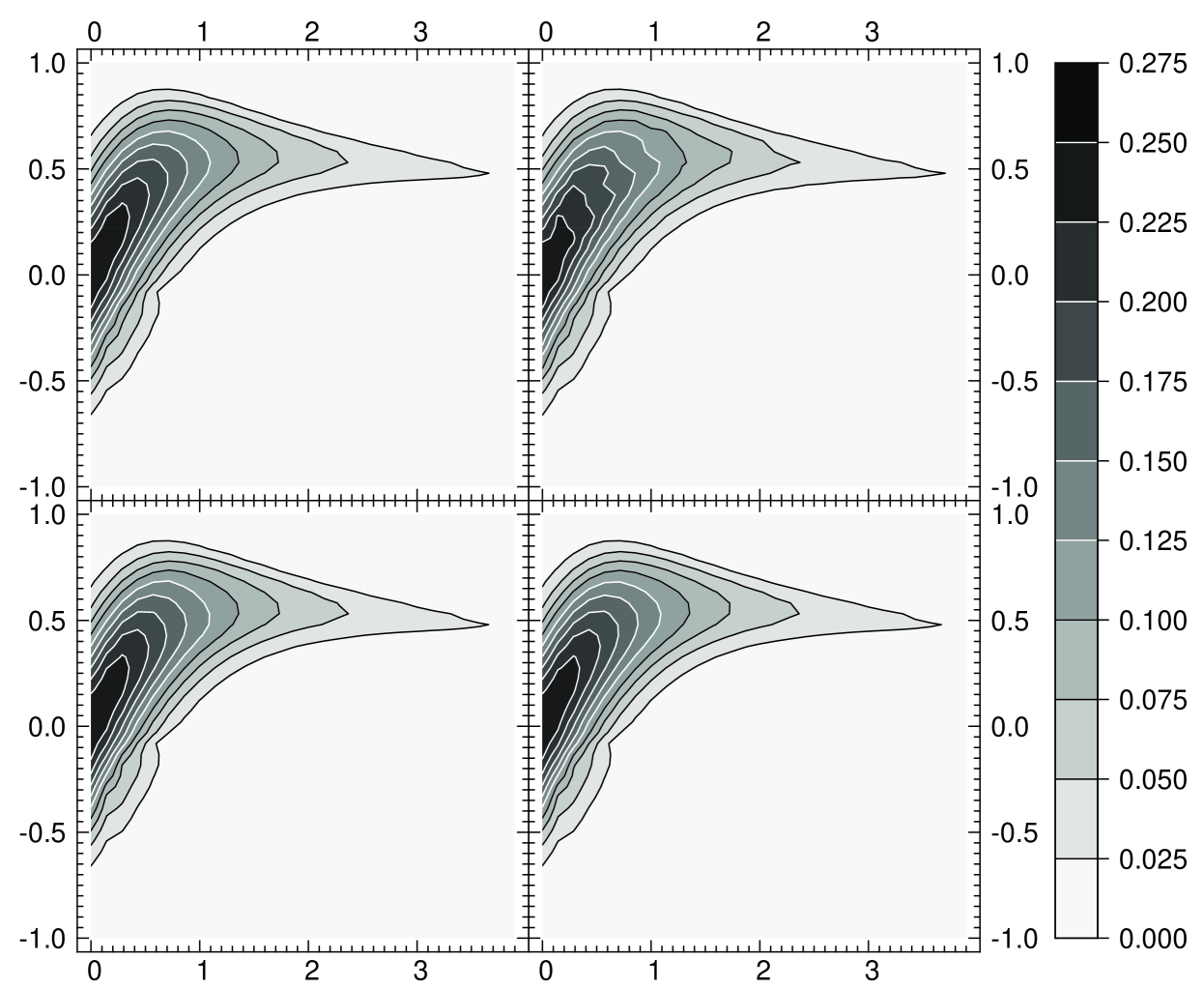
Figure 1: Fit of $F_{\phi}$ (as described in section 4) with various penalizing functions. From top-left to bottom-right: (1) original $F_{\phi}$ and $F_{\phi}$ restored by (2) MEM with uniform prior, (3) MEM with floating smooth prior and (4) quadratic regularisation, i.e. $R_{\mathrm{quad}}$ with $n=1$ as defined in Eq. 18. As expected, no significant difference is to be found in the fits, though in panel (2), $F_{\phi}$ is slightly rougher. The SNR is 50.

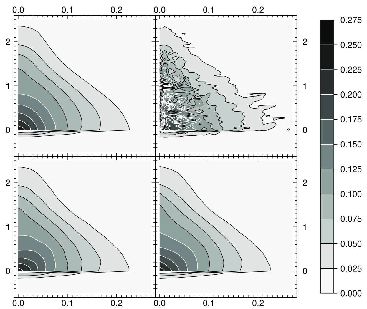
Figure 2: Restoration of $\hat{f}(\eta,h)$ from Fig. 1 (from top-left to bottom-right): (1) true distribution and distributions restored by (2) MEM with uniform prior, (3) MEM with smooth floating prior and (4) quadratic regularisation, i.e.  $R_{\mathrm{quad}}$ with $n=1$ as defined in Eq. 18. Note that MEM with a uniform prior yields a rather unsmooth solution, which is expected since no penalty is imposed by this method for lack of smoothness.

3 Numerical optimisation

In the previous section it was shown that the inversion problem reduces to the minimisation of a multi-dimensional function $Q({\textbf{{f}}})=L({\textbf{{f}}})+\mu{}R({\textbf{{f}}})$ with respect to a great number of parameters (from a few $10^{4}$ to $10^{6}$) and subject to the constraints that (i) the likelihood term keeps some target value: $L({\textbf{{f}}})=N_{\mathrm{e}}$, (ii) all parameters remain positive and that (iii) special care is taken along some physical boundaries. Unfortunately there exists no general black-box algorithm able to perform this kind of optimisation.

Let us therefore investigate in turns three techniques to carry the minimisation of increasing efficiency and complexity: direct methods, iterative minimisation along a single direction (accounting for positivity at fixed regularisation) and iterative minimisation with a floating regularisation weight.

3.1 Linear solution

Using quadratic regularisation, the problem is solved by minimizing:

$$Q_{\mathrm{quad}}({\textbf{{f}}})={(\tilde{{\textbf{{F}}}}-{\textbf{{a}}}\!\cdot\!{\textbf{{f}}})^{\bot}}\!\cdot\!{\textbf{{W}}}\!\cdot\!(\tilde{{\textbf{{F}}}}-{\textbf{{a}}}\!\cdot\!{\textbf{{f}}})+\mu\,{{\textbf{{f}}}^{\bot}}\!\cdot\!{\textbf{{K}}}\!\cdot\!{\textbf{{f}}}\,.$$ (22)

where W is the inverse of the covariance matrix of the data. The solution ${\textbf{{f}}}_{\mathrm{quad}}$ which minimises $Q_{\mathrm{quad}}$ is:

$${\textbf{{f}}}_{\mathrm{quad}}=({{\textbf{{a}}}^{\bot}}\!\cdot\!{\textbf{{W}}}\!\cdot\!{\textbf{{a}}}+\mu\,{\textbf{{K}}})^{-1}\!\cdot\!{{\textbf{{a}}}^{\bot}}\!\cdot\!{\textbf{{W}}}\!\cdot\!{\textbf{{F}}}\,.$$ (23)

This solution, which is linear with respect to the data, is clearly not constrained to be positive.

3.2 Non linear optimisation

Linear methods only provide raw, possibly locally negative, solutions. At the very least, enforcing positivity of the solution – and more generally if the penalised function is not quadratic – requires non-linear minimisation. In that case, the minimisation of $Q({\textbf{{f}}})$ must be carried out by successive approximations.

At the $n^{\mathrm{th}}$ step, such iterative minimisation methods usually proceed by varying the current parameters ${\textbf{{f}}}^{(n)}$ along a direction $\delta{\textbf{{f}}}^{(n)}$ so as to minimise $Q$; the new estimate of the parameters reads:

$${\textbf{{f}}}^{(n+1)}={\textbf{{f}}}^{(n)}+\lambda^{(n)}\,\delta{\textbf{{f}}}^{(n)}\,,$$ (24)

where the optimum step size $\lambda^{(n)}$ is the scalar:

$$\lambda^{(n)}=\arg\{\min_{\lambda}[Q({\textbf{{f}}}^{(n)}+\lambda\,\delta{\textbf{{f}}}^{(n)})]\}\,.$$ (25)

The problem being to choose suitable successive directions of minimisation.

3.2.1 Optimum direction of minimisation

In principle, the optimum direction of minimisation $\delta{\textbf{{f}}}$ could be derived from the Taylor’s expansion:

$$Q({\textbf{{f}}}+\delta{\textbf{{f}}})\simeq Q({\textbf{{f}}})+\sum_{k}\delta\!f_{k}\frac{\partial{}Q}{\partial{}f_{k}}+\frac{1}{2}\sum_{k,l}\delta\!f_{k}\delta\!f_{l}\frac{\partial^{2}Q}{\partial{}f_{k}\partial{}f_{l}}\,,$$ (26)

that is minimised for the step

$$\delta{\textbf{{f}}}=-\bigl{(}\nabla\!\nabla\!Q\bigr{)}^{-1}\!\cdot\!\nabla\!Q\,,$$ (27)

where $\nabla\!Q$ and $\nabla\!\nabla\!Q$ are respectively the gradient vector and the Hessian matrix of $Q({\textbf{{f}}})$:

$$\nabla\!Q_{k}=\frac{\partial{}Q}{\partial{}f_{k}}\,,\quad\mbox{and}\quad\nabla\!\nabla\!Q_{k,l}=\frac{\partial^{2}Q}{\partial{}f_{k}\partial{}f_{l}}\,.$$

The whole difficulty of multi-dimensional minimisation deals with estimating the inverse of the Hessian matrix, which may generically be too large to be computed and stored. A further difficulty arises when $Q({\textbf{{f}}})$ is highly non-quadratic (e.g.  in MEM) since the behaviour of $Q({\textbf{{f}}})$ can significantly differ from that of its Taylor’s expansion.

There exist a number of multi-dimensional minimisation numerical routines that avoid the direct computation of the inverse of the Hessian matrix: e.g. steepest descent, conjugate gradient algorithm, Powell’s method, etc. [Press et al., 1988]. For the steepest descent method, the direction of minimisation is simply given by the gradient: $\delta{\textbf{{f}}}_{\mathrm{SD}}=-\nabla\!Q$. Other more efficient multi-dimensional minimisation methods attempt to build information about the Hessian while deriving a more optimal direction, i.e.  a better approximation of $-(\nabla\!\nabla\!Q)^{-1}\!\cdot\!\nabla\!Q$. For instance, the conjugate-gradient method builds a series of optimum conjugate directions $\delta{\textbf{{f}}}_{\mathrm{CG}}$, each of which is a linear combination of the current gradient and the previous direction [Press et al., 1988]. Among those improved methods and when the number of parameters is very large, the choice of conjugate-gradient is driven by its efficiency both in terms of convergence rate and memory allocation.

3.2.2 Accounting for positivity

Let us now examine the non-linear strategy leading to a minimisation of $Q({\textbf{{f}}})$ with the constraint that $\hat{f}(\eta,h)\geq 0$ everywhere. We will assume that the basis of functions $\{\hat{e}_{k}(\eta,h)\}$ is chosen so that the positivity constraint is equivalent to enforcing that $f_{k}\geq 0;\forall{}k$ (see Appendix A for an example of such a basis).

When seeking the appropriate step size given by Eq. (25), it is possible to account for positivity by limiting the range of $\lambda^{(n)}$:

$${\textbf{{f}}}^{(n+1)}\geq 0\quad\Leftrightarrow\quad-\mathrel{\mathop{{\mathrm{min}}}\limits_{\delta\!f^{(n)}_{k}>0}}\frac{f^{(n)}_{k}}{\delta\!f^{(n)}_{k}}\leq\lambda^{(n)}\leq-\mathrel{\mathop{{\mathrm{max}}}\limits_{\delta\!f^{(n)}_{k}<0}}\frac{f^{(n)}_{k}}{\delta\!f^{(n)}_{k}}.$$

In practice this procedure blocks the steepest descent method long before the right solution is found. It is in fact better to truncate negative values after each step:

$$f_{k}^{(n+1)}=\max\{0,f_{k}^{(n)}+\lambda^{(n)}\,\delta{}f_{k}^{(n)}\}\,.$$

Besides, any of these methods to enforce positivity breaks conjugate-gradient minimisation since this latter assumes that the true minimum of $Q({\textbf{{f}}}^{(n)}+\lambda^{(n)}\,\delta{\textbf{{f}}}^{(n)})$ is reached while varying $\lambda^{(n)}$.

Thiébaut & Conan [Thiébaut & Conan, 1995] circumvent this difficulty thanks to a reparametrisation that enforces positivity. Following their argument, $Q$ is minimised here with respect to a new set of parameters x such as:

$$f_{k}=g(x_{k})\,,\quad\mbox{with $g:{\mathrm{I\!R}}\mapsto{\mathrm{I\!R}}_{+}$}\,.$$ (28)

The following various reparametrisations meet these requirements:

$$\begin{array}[]{lcl}f_{k}=\mathrm{exp}(x_{k})&\Rightarrow&g^{\prime}(x_{k})^{2}=f_{k}^{2}\,,\\ f_{k}=x_{k}^{2n}\quad\mbox{($n$ positive integer)}&\Rightarrow&g^{\prime}(x_{k})^{2}\propto f_{k}^{2-1/n}\,.\\ \end{array}$$

When $Q({\textbf{{f}}})$ is quadratic, $Q({\textbf{{f}}}+\lambda\delta{\textbf{{f}}})$ is a second order polynomial with respect to $\lambda$, the minimisation of which can trivially be performed with a very limited number of matrix multiplications. One drawback of the reparametrisation is that, since $g(\cdot)$ is non-linear, $Q\!\circ\!g({\textbf{{x}}})$ is necessarily non-quadratic. In that case the exact minimisation of $Q\!\circ\!g({\textbf{{x}}}+\lambda\delta{\textbf{{x}}})$ – mandatory in conjugate gradient or Powell’s methods – requires many more matrix multiplications. Another drawback is that the direction of investigation derived by conjugate gradient or Powell’s methods may be no longer optimal requiring many more steps to obtain the overall solution. This latter point follows from the fact that these methods collect information about the Hessian while taking into account the previous steps, whereas for a non-quadratic functional this information becomes obsolete very soon since the Hessian (with respect to x) is no longer constant [Skilling & Bryan, 1984].

Consequently, instead of varying the parameters x, we propose to derive a step $\delta{\textbf{{f}}}$ for varying f from the reparametrisation that enforces positivity. Let $\delta{\textbf{{x}}}$ be the chosen direction of minimisation for x, the sought parameters reads: $g(x_{k}+\lambda\,\delta{}x_{k})\simeq{}f_{k}+\lambda\,\delta{}x_{k}\,g^{\prime}(x_{k})$. Identifying the right hand side of this expression with $f_{k}+\lambda\delta\!f_{k}$ yields: $\delta\!f_{k}=\delta{}x_{k}\,g^{\prime}(x_{k})$. Using the steepest descent direction:

$$\delta{}x_{k}=-\frac{\partial{}Q}{\partial{}x_{k}}=-\frac{\partial{}Q}{\partial{}f_{k}}g^{\prime}(x_{k})\,.$$

yielding finally:

$$\delta\!f_{k}=-\frac{\partial{}Q}{\partial{}f_{k}}g^{\prime}(x_{k})^{2}\,=-\frac{\partial{}Q}{\partial{}f_{k}}f_{k}^{\nu}\,,$$ (29)

with $1\leq\nu\leq 2$ depending on the particular choice of $g(\cdot)$.

3.2.3 Algorithm for 1D minimisation: positivity at fixed $\mu$

In Appendix B we show that other authors have derived very similar optimum direction of minimisation but in the more restrictive case of a regularisation by $R_{\mathrm{MEM}}$. Note that our approach is not limited to this type of penalising function since positivity is enforced extrinsically. In short, the minimisation step is derived from the unifying expression:

$$\delta\!f_{k}=-q_{k}\nabla\!Q_{k}\,,$$ (30)

where the gradient is scaled by (see Appendix B):

$$q_{k}=\left\{\begin{array}[]{cl}f_{k}^{\nu}\,,&\mbox{this work (with $1\leq\nu\leq 2$)}\,,\\[3.01385pt] f_{k}\,,&\mbox{Richardson-Lucy}\,,\\[3.01385pt] f_{k}/\mu\,,&\mbox{classical MEM}\,,\\[5.16663pt] {\displaystyle\frac{f_{k}}{\mu+f_{k}\sum\limits_{i,j}\frac{a_{i,j,k}^{2}}{{\mathrm{Var}}(\tilde{F}_{i,j})}}}\,,&\mbox{Cornwell-Evans.}\\ \end{array}\right.$$

The scheme of the 1D-optimisation algorithm is illustrated in Fig. 3. Iterations are stopped when the decrement in $Q({\textbf{{f}}})$ becomes negligible, i.e. when:

$${\left|{Q({\textbf{{f}}}+\lambda\delta{\textbf{{f}}})-Q({\textbf{{f}}})}\right|}\leq\epsilon\,{\left|{Q({\textbf{{f}}})}\right|}\,,$$

where $\epsilon>0$ is a small number which should not be smaller than the square root of the machine precision [Press et al., 1988]. Lucy [Lucy, 1994] has suggested another stop criterion based on the value of the ratio:

$$\rho={\left|{{\left|{\delta{\textbf{{f}}}}\right|}}\right|}\,/\,({\left|{{\left|{\delta{\textbf{{f}}}_{\mathrm{L}}}\right|}}\right|}+{\left|{{\left|{\delta{\textbf{{f}}}_{\mathrm{R}}}\right|}}\right|})\,,$$

where $\delta{\textbf{{f}}}_{\mathrm{L}}$ and $\delta{\textbf{{f}}}_{\mathrm{R}}$ are the directions which minimise the likelihood and the regularisation terms:

$$\delta{\textbf{{f}}}_{\mathrm{L}}=-{\textbf{{q}}}\times\nabla\!L\quad\mbox{and}\quad\delta{\textbf{{f}}}_{\mathrm{R}}=-\mu{\textbf{{q}}}\times\nabla\!R\,,$$

where $\times$ denotes element-wise product (in other words q stands loosely for ${\mathrm{Diag}}(q_{1},\ldots,q_{n})$). In practice and regardless of the particular choice for q, the algorithm makes no significant progress when $\rho$ becomes smaller than $10^{-5}$.

Figure 3: Synopsis of the single direction minimisation algorithm.. Here $\epsilon_{1}\simeq 10^{-8}$ and $\epsilon_{2}\simeq 10^{-5}$.

3.2.4 Performance issues

During the tests, it was found that conjugate-gradient method with reparametrisation and iterative methods with direction given by Eq. (30) require roughly the same number of steps (one step involving minimisation along a new direction of minimisation). Yet the non-linear reparametrisation required to enforce positivity in conjugate gradient method prevents interpolation and in effect spends much more time (a factor of 10 to 20) to perform line minimisation. Besides, when the current estimate is far from the solution, minimisation direction following our prescription (29) or that of classical MEM or Lucy spends fewer steps than that of Cornwell & Evans to bring f near the true solution. When the current estimate is sufficiently close to the solution, Cornwell & Evans’s method spends half as many steps as the other methods to reach the solution. The best compromise is to start with $\delta\!f_{k}\propto-f_{k}\nabla\!Q_{k}$, then after some iterations use $\delta{\textbf{{f}}}=\delta{\textbf{{f}}}_{\mathrm{CE}}$. As a rule of thumb, for low signal-to-noise ratios (${S\!N\!R}\sim 5$) about as many steps as number of parameters are required, for high signal-to-noise ratios (${S\!N\!R}\geq 30$) fewer steps are needed (up to 10 times less). It remains that with these methods trial and error iterations are required to find the appropriate value for $\mu$. The different implementations are illustrated and compared in Fig. 1 and  2 as described in section (4).

Accounting for positivity in multi-dimensional optimisation therefore leads to a modified steepest descent algorithm for which the current gradient is locally rescaled. A faster convergence is achieved when some information from the Hessian is extracted appropriately. Yet, the above described algorithm assumes that optimisation is performed with a fixed value of the Lagrange parameter $\mu$. Let us now turn to a more general minimisation along several direction which allow $\mu$ to be adjusted on the fly during the minimisation.

3.3 Minimisation along several directions

3.3.1 Skilling & Bryan method revisited

In the context of maximum entropy image restoration, Skilling & Bryan [Skilling & Bryan, 1984] (hereinafter SB) have proposed a powerful method which is both efficient in optimising a non-linear problem with a great number of parameters and able to vary automatically the weight of regularisation so that the sought solution satisfies $L({\textbf{{f}}})=N_{\mathrm{e}}$. Here their approach is further generalise to any penalising function. In short, SB derive their method from the following remarks:

1. To account for positivity, they suggest an appropriate “metric” (or rescaling) which is equivalent to multiplying each minimisation direction by ${\textbf{{q}}}={\textbf{{f}}}$.

2. The regularisation weight $\mu$ is adjusted at each iteration to meet the constraint $L({\textbf{{f}}})=N_{\mathrm{e}}$. Therefore, instead of minimising along the single direction $-{\textbf{{q}}}\times(\nabla\!L+\mu\nabla\!R)$, at least two directions are considered: $-{\textbf{{q}}}\times\nabla\!L$ and $-{\textbf{{q}}}\times\nabla\!R$.

3. Since the Hessian is not constant – at least since $\mu$ is allowed to vary, no information is carried from the previous iterations. This clearly excludes conjugate-gradient or similar optimisation methods, but favours non-quadratic penalising functions for which the Hessian is not assumed to be constant.

4. If the whole Hessian cannot be computed, it can nevertheless be applied to any vector e of same size as f in a finite number of operations, e.g.  two matrix multiplications for the likelihood term: $\nabla\!\nabla\!L\!\cdot\!{\textbf{{e}}}=2\,{{\textbf{{a}}}^{\bot}}\!\cdot\!({\textbf{{a}}}\!\cdot\!{\textbf{{e}}})$ (where, for the sake of simplicity, the diagonal weighting matrix was omitted here). They illustrate how this provide a means to include some knowledge from the local Hessian while seeking the optimum minimisation direction.

3.3.2 Local minimisation sub-space

In order to adjust the regularisation weight, at least two simultaneous directions of minimisation should be used: $-{\textbf{{q}}}\times\nabla\!L$ and $-{\textbf{{q}}}\times\nabla\!R$. Furthermore, the local Hessian provides other directions of minimisation to increase the convergence rate. Using matrix notation, the Taylor expansion of $Q({\textbf{{f}}})$ for two simultaneous directions $\delta{\textbf{{f}}}_{1}$ and $\delta{\textbf{{f}}}_{2}$ reads:

$$Q({\textbf{{f}}}\!+\!\delta{\textbf{{f}}}_{1}\!+\!\delta{\textbf{{f}}}_{2}) \!\!\simeq\!\! Q({\textbf{{f}}})+\delta{{\textbf{{f}}}_{1}^{\bot}}\!\!\cdot\!\!\nabla\!Q+\frac{1}{2}\delta{{\textbf{{f}}}_{1}^{\bot}}\!\!\cdot\!\nabla\!\nabla\!Q\!\cdot\!\delta{\textbf{{f}}}_{1}$$

$$+\delta{{\textbf{{f}}}_{2}^{\bot}}\!\!\cdot\![\nabla\!Q+\nabla\!\nabla\!Q\!\cdot\!\delta{\textbf{{f}}}_{1}]+\frac{1}{2}\delta{{\textbf{{f}}}_{2}^{\bot}}\!\!\cdot\!\nabla\!\nabla\!Q\!\cdot\!\delta{\textbf{{f}}}_{2}\,,$$

where the Hessian and gradient are evaluated at f. Given a first direction $\delta{\textbf{{f}}}_{1}$, the optimal choice for a second direction is:

$$\delta{\textbf{{f}}}_{2,{\mathrm{opt}}}=-(\nabla\!\nabla\!Q)^{-1}\!\cdot\!(\nabla\!Q+\nabla\!\nabla\!Q\!\cdot\!\delta{\textbf{{f}}}_{1})\,.$$

In MEM, recall that positivity is enforced explicitly by the regularisation penalty function while efficient minimisation methods rely on the approximation of $(\nabla\!\nabla\!Q)^{-1}$ by a scaling vector q. The optimum first two directions then become in MEM:

$$\delta{\textbf{{f}}}_{1,{\mathrm{opt}}}\simeq-{\textbf{{q}}}\times\nabla\!Q\,,\quad\mbox{and}\quad\delta{\textbf{{f}}}_{2,{\mathrm{opt}}}\simeq-{\textbf{{q}}}\times(\nabla\!Q+\nabla\!\nabla\!Q\!\cdot\!\delta{\textbf{{f}}}_{1})\,,$$

Since the first term in the right hand side expression of $\delta{\textbf{{f}}}_{2,{\mathrm{opt}}}$ is $\delta{\textbf{{f}}}_{1,{\mathrm{opt}}}$, the two near optimum directions sought are finally:

$$\delta{\textbf{{f}}}_{1}=-{\textbf{{q}}}\times\nabla\!Q\,,\quad\mbox{and}\quad\delta{\textbf{{f}}}_{2}=-{\textbf{{q}}}\times(\nabla\!\nabla\!Q\!\cdot\!\delta{\textbf{{f}}}_{1})\,.$$ (31)

Similar considerations yield here further possible directions:

$$\delta{\textbf{{f}}}_{n}=-{\textbf{{q}}}\times(\nabla\!\nabla\!Q\!\cdot\!\delta{\textbf{{f}}}_{n-1})\,.$$ (32)

If the rescaling, q, provides too good an approximation of the inverse of the Hessian, then $\delta{\textbf{{f}}}_{1}$ and $\delta{\textbf{{f}}}_{2}$ would almost be identical (i.e. antiparallel); hence using only one is sufficient. In other words, since the local Hessian is accounted for by the use of additional directions of minimisation, there is no need that ${\mathrm{Diag}}({\textbf{{q}}})$ be an accurate approximation of $(\nabla\!\nabla\!Q)^{-1}$. The crude rescaling given by Eq. (51) is therefore sufficient, i.e.  taking: ${\textbf{{q}}}={\textbf{{f}}}$. This definition of q has the further advantage to warrant positive values of f and does not depend on the actual value of $\mu$ (which is obviously not the case for the Hessian).

If no term in $Q({\textbf{{f}}})$ enforces positivity, it was shown earlier that the reparametrisation (28) would. From the Taylor expansion of $Q({\textbf{{x}}})$, the first two steepest descent directions with respect to the parameters x are given by:

$$\delta{}x_{1,k} \!=\! -\frac{\partial{}Q}{\partial{}x_{k}}\!=\!-g^{\prime}(x_{k})\nabla\!Q_{k}\,,$$ (33)

$$\delta{}x_{2,k} \!=\! -\sum_{l}\frac{\partial^{2}Q}{\partial{}x_{k}\partial{}x_{l}}\frac{\partial{}Q}{\partial{}x_{l}}\!=\!-g^{\prime}(x_{k})\sum_{l}\nabla\!\nabla\!Q_{k,l}g^{\prime}(x_{l})\delta{}x_{1,l}\,.$$

Since $\delta{}f_{k}\simeq{}g^{\prime}(x_{k})\delta{}x_{k}$, the near two optimum directions of minimisation for the parameters f read:

$$\delta{}f_{1,k} = -g^{\prime}(x_{k})^{2}\nabla\!Q_{k}\,,$$ (34)

$$\delta{}f_{2,k} = -g^{\prime}(x_{k})^{2}\sum_{l}\nabla\!\nabla\!Q_{k,l}\delta{}f_{1,l}\,,$$ (35)

which are incidentally identical to those given by Equation (31), provided that $q_{k}=g^{\prime}(x_{k})^{2}$.

For all the regularisation penalising functions considered here, clearly the best choice is to use directions given by the Hessian applied to Eq. (33) when other directions of minimisation than those related to the gradient are considered. Since $\mu$ can vary, the Hessians of $L$ and $R$ have to be applied separately. At each step, the minimisation is therefore performed in the $n=3\times 2=6$ dimensional sub-space defined by:

$$\begin{array}[]{ll}\delta{\textbf{{f}}}_{1}=-{\textbf{{q}}}\times\nabla\!L\,,&\delta{\textbf{{f}}}_{2}=-{\textbf{{q}}}\times\nabla\!R\,,\\ \delta{\textbf{{f}}}_{3}=-{\textbf{{q}}}\times(\nabla\!\nabla\!L\!\cdot\!\delta{\textbf{{f}}}_{1})\,,&\delta{\textbf{{f}}}_{4}=-{\textbf{{q}}}\times(\nabla\!\nabla\!L\!\cdot\!\delta{\textbf{{f}}}_{2})\,,\\ \delta{\textbf{{f}}}_{5}=-{\textbf{{q}}}\times(\nabla\!\nabla\!R\!\cdot\!\delta{\textbf{{f}}}_{1})\,,&\delta{\textbf{{f}}}_{6}=-{\textbf{{q}}}\times(\nabla\!\nabla\!R\!\cdot\!\delta{\textbf{{f}}}_{2})\,,\\ \end{array}$$ (36)

where

$$q_{k}=f_{k}^{\nu}\quad\mbox{with}\quad 1\leq\nu\leq 2\,.$$ (37)

When $\nu=1$, q is the same metric as that introduced by SB while relying on other arguments. Depending on the actual expression for $\nabla\!\nabla\!R$ (and in particular in MEM with a constant prior), a smaller number of directions need be explored (for instance, SB used only $n=3$ simultaneous directions since when ${\textbf{{q}}}={\textbf{{f}}}$, $\nabla\!\nabla\!R=1/{\textbf{{f}}}$ so $\delta{\textbf{{f}}}_{5}=\delta{\textbf{{f}}}_{1}$, $\delta{\textbf{{f}}}_{6}=\delta{\textbf{{f}}}_{2}$; they also use a linear combination of $\delta{\textbf{{f}}}_{3}$ and $\delta{\textbf{{f}}}_{4}$). In this $n$-dimensional sub-space, a simple second order Taylor expansion of $Q({\textbf{{f}}}+\sum_{i=1}^{n}\lambda_{i}\delta{\textbf{{f}}}_{i})$, shows that the optimum set of weights sought, $\{\lambda_{1},...,\lambda_{n}\}$, is given by the solution of the $n$ linear equations parametrised by $\mu$ and given by:

$$\sum_{j=1}^{n}\lambda_{j}\delta{{\textbf{{f}}}^{\bot}}_{j}\!\cdot\!(\nabla\!\nabla\!L+\mu\nabla\!\nabla\!R)\!\cdot\!\delta{\textbf{{f}}}_{i}=-\delta{{\textbf{{f}}}^{\bot}}_{i}\!\cdot\!(\nabla\!L+\mu\nabla\!R)\,.$$ (38)

Now in that sub-space, the optimisation may be ill-conditioned (i.e. the set of linear equations are linearly dependent in a numerical sense). In order to deal with this degeneracy truncated SVD decomposition [Press et al., 1988] is used to find a set of numerically independent directions. In practice, the rank of the 6 linear equations varies from 2 (very far from the solution or when convergence is almost reached) to typically 5 or 6. This method turns out to be much easier to implement than the bi-diagonalisation suggested by SB.

3.3.3 On the fly derivation of the regularisation weight

At each iteration a strategy similar to that of SB was adopted here to update the value of $\mu$:

1. $L_{\mathrm{min}}$ and $L_{\mathrm{max}}$ are the values of the likelihood term in the sub-space in the limits $\mu\rightarrow 0$ and $\mu\rightarrow\infty$ respectively. The corresponding solutions give what we call the maximum likelihood solution and the maximum regularised solution in the sub-space.

2. If $L_{\mathrm{max}}<N_{\mathrm{e}}$ the maximum regularised solution corresponding to $L_{\mathrm{max}}$ is adopted to proceed to the next iteration. Otherwise, in order to avoid relaxing the regularisation and following SB, a modest reachable goal is fixed:

   $$L_{\mathrm{aim}}={\mathrm{max}}\{N_{\mathrm{e}},(1-\alpha)L_{\mathrm{prev}}+\alpha{}L_{\mathrm{min}}\}$$

   where $L_{\mathrm{prev}}$ is the likelihood value at the end of the previous iteration, while $0\!<\!\alpha\!<\!1$ (say $\alpha=2/3$). A simple bi-section method is applied to seek the value of $\mu$ for which the solution of Eq. (38) yields $L=L_{\mathrm{aim}}$.

Following this scheme, the algorithm varies the value of $\mu$ so that at each iteration the likelihood is reduced until it reaches its target value; then the regularisation term is minimised while the likelihood remains constant.

As a stop criteria, a measure of the statistical discrepancy between two successive iterations:

$$\sum_{k}f^{(n)}_{k}{\left|{f^{(n+1)}_{k}-f^{(n)}_{k}}\right|}\quad/\quad\sum_{k}f^{(n)}_{k}\,,$$

is computed. In practice, in order to avoid over-regularisation, $N_{\mathrm{e}}$ is taken to be $N_{\mathrm{data}}-\sqrt{2N_{\mathrm{data}}}$. The corresponding scheme of the $n$-dimensional optimisation algorithm is illustrated in Fig. 4.

Figure 4: Synopsis of the multiple directions multidimensional minimisation algorithm with adjustment of the regularisation weight. In this algorithm, $f_{\mathrm{min}}>0$ is a small threshold used to avoid negative values, $0\leq\epsilon\ll 1$ is a small value used to check convergence.

3.3.4 Performance & assessments

The optimisation of $Q({\textbf{{f}}})$ in a multi-dimensional sub-space yields many practical advantages: (i) it provides faster convergence rates (about 10 times less overall iterations and even much less when accounting for the number of inversions required to derive the regularisation weight) and less overall cpu time in spite of the numerous matrix multiplications involved to compute the $n$ directions of minimisation and their images by the Hessians. (ii) It yields a more robust algorithm because it is less sensitive to local minima and also because the routine requires less tuning. (iii) Since $\mu$ varies between iterations and since the local Hessian is always re-estimated, the solution can be modified on the fly, e.g. rescaled, without perturbing the convergence. Hence the normalisation is no more an issue.

This algorithm presents the following set of improvements over that of Skilling & Bryan: (i) a more general penalising functions than entropy is considered (e.g.  entropy with floating prior or quadratic penalising function) which yield a different metric derived heuristically. This yields almost the same optimisation sub-space but from a different approach; (ii) truncated SVD is implemented to avoid ill-conditioned problems in this minimisation sub-space.

4 Simulations

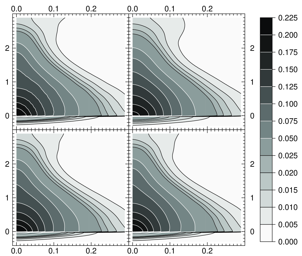
Figure 5: (from top-left to bottom-right): (1) true distribution (approximately that of a disk with Toomre parameter $Q=1.25$) and mean restoration of $\hat{f}(\eta,h)$ out of 40 itterations for a SNR of 5 (2), 30 (3) and 100 (4). Abscissa is normalised specific energy $\eta$ and ordinate is specific angular momentum $h$. Note that the isocontours are not sampled uniformly in order to display more acurately counter rotating stars.

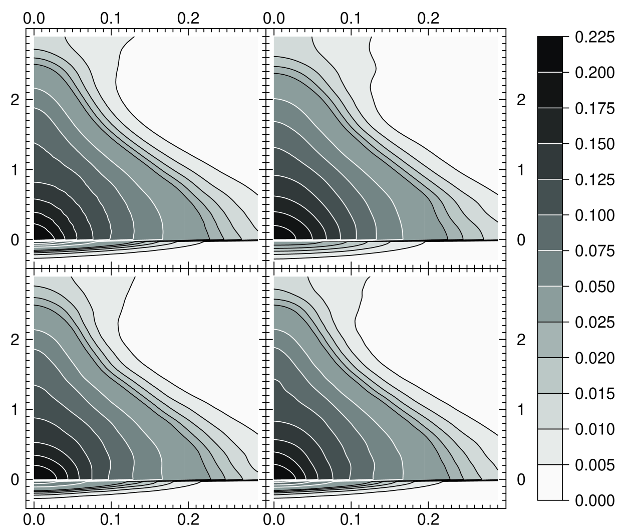
Figure 6: true distribution and one sample for each SNR out of the 40 restorations carried out, displayed as in Fig. 5. Abscissa is normalised specific energy $\eta$ and ordinate is specific angular momentum $h$. Comparison with Fig. 5 shows that the inversion is successfull both statistically and on a per sample basis.

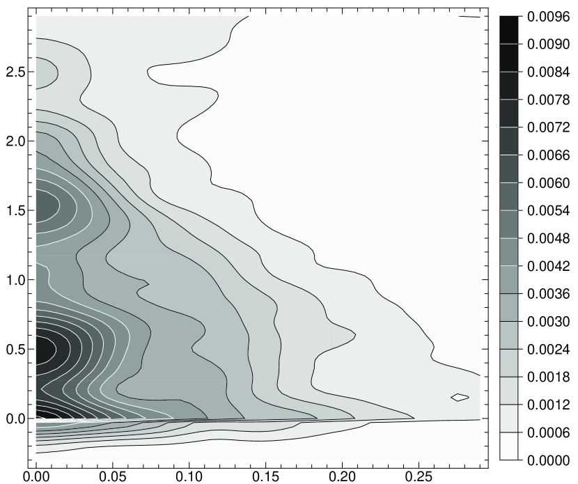
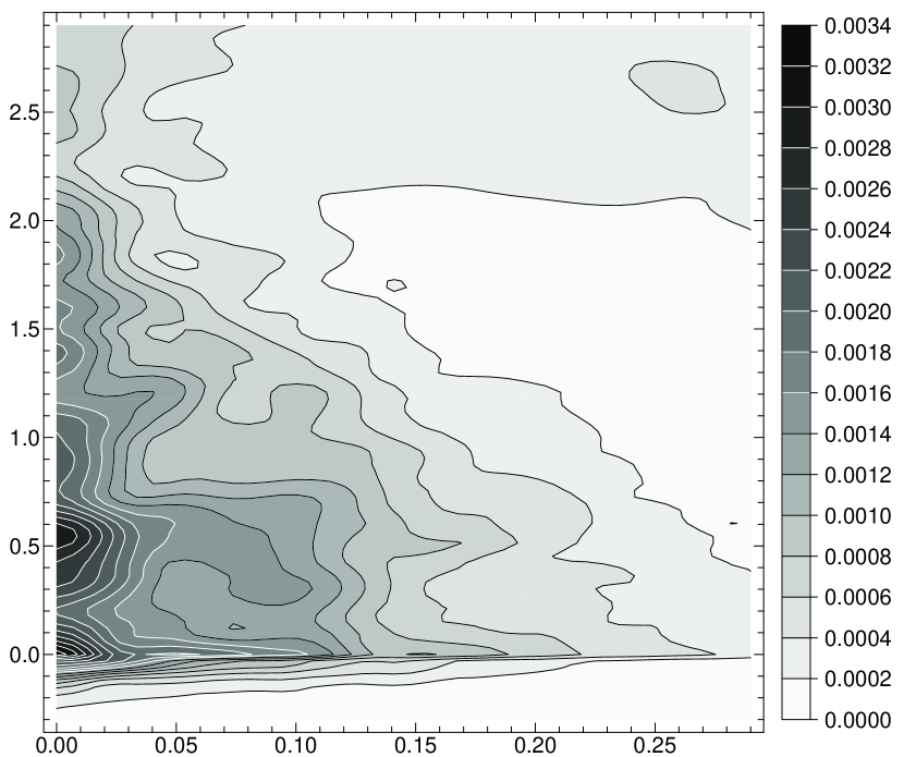
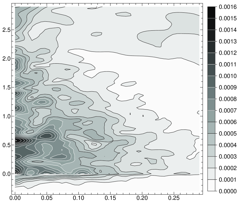
Figure 7: Standard deviation for each SNR out of the 40 restorations carried out displayed as in Fig. 5. From top to bottom: ${S\!N\!R}=5$, ${S\!N\!R}=30$ and ${S\!N\!R}=100$. Abscissa is normalised specific energy $\eta$ and ordinate is specific angular momentum $h$. Note that the maximum residual error is well below the signal’s amplitude and decreasing with increasing SNR.

4.1 Specificities of stellar disk inversion

4.1.1 Models of azimuthal velocity distributions.

Simulated azimuthal velocity distributions can be constructed via the prescription described in Pichon & Lynden-Bell [Pichon & Lynden-Bell, 1996]. The construction of Gaussian line profiles compatible with a given temperature requires specifying the mean azimuthal velocity of the flow, $\left\langle v_{\phi}\right\rangle$ on which the Gaussian should be centered, the surface density, $\Sigma(R)$ and the azimuthal velocity dispersion $\sigma_{\phi}$. The line profile $F$ then reads

$$F_{\phi}(R,v_{\phi})={\Sigma(R)\over\sqrt{2\pi}\,\sigma_{\phi}}\,\exp\left(-{\left[v_{\phi}-\left\langle v_{\phi}\right\rangle\right]^{2}\over 2\sigma_{\phi}^{2}}\right)\,.$$ (39)

Here the azimuthal velocity dispersion is related to the azimuthal pressure, $p_{\phi}$, by

$$\sigma_{\phi}^{2}=p_{\phi}/\Sigma-\left\langle v_{\phi}\right\rangle^{2}\,.$$ (40)

The azimuthal pressure $p_{\phi}$ follows from the equation of radial support,

$$\left\langle v_{\phi}^{2}\right\rangle-R{\partial\psi\over\partial R}={\partial\left(R\Sigma\sigma_{R}^{2}\right)\over\Sigma\,\partial R}\,,$$ (41)

and the kinematical “temperature” of the disk with a given Toomre number $Q$ [Toomre, 1964].

$$Q=0.298\,\sigma_{R}\kappa\,/\,\Sigma\,.$$ (42)

The expression of the average azimuthal velocity, $\langle v_{\phi}\rangle$, may be taken to be that which leads to no asymmetric drift equation:

$$\Sigma\left\langle v_{\phi}\right\rangle^{2}=p_{\phi}-p_{R}(\kappa\,R\,/\,2v_{c})^{2}\,,$$ (43)

where $\kappa$ is the epicyclic frequency, and $v_{c}$ the velocity of circular orbits. Equations (39)–(43) provide a prescription for the Gaussian azimuthal line profile $F_{\phi}$. These azimuthal velocity distributions are used throughout to generate simulated data corresponding to iso-Q Kuzmin disk.

4.1.2 The counter-rotating radial orbits

As shown in Fig. 1, the azimuthal distributions of our models have Gaussian tails corresponding to stars on almost radial orbits with small negative azimuthal velocity. These few stars play a strong dynamical role in stabilising the disk, and as such should not be overlooked since they significantly increase the azimuthal dispersion of inner orbits, effectively holding the inner galaxy against its self-gravity. Now this Gaussian tail translates in the momentum, reduced energy space as a small group of counter rotating orbits introducing a cusp in the number of stars near $h=0$ (this cusp is only apparent since the distribution is clearly continuous and differentiable across this line). In practice the regularisation constraint across $h=0$ is relaxed, treating in effect independently the two regions.

4.2 Validation & efficiency

4.2.1 Quality estimation

Clearly the quality level for the reconstructed distribution will depend upon the application in mind. For stability analysis, the relevant information involves for instance its gradients in action space. An acute quality estimator would therefore involve such gradients, though their computation requires some knowledge of the orbital structure of the disk, and is beyond the scope of this paper. Here the quality of the reconstruction is estimated while computing the mean distribution-weighted residual between the distribution sought and the model recovered. It is defined by:

$${\mathrm{error}}({\textbf{{f}}})\!\!=\!\!\left\langle|f-f_{\mathrm{true}}|\right\rangle\!\!\simeq\!\!\frac{\sum_{i}f_{{\mathrm{true}},i}\,|f_{i}-f_{{\mathrm{true}},i}|}{\sum_{i}f_{{\mathrm{true}},i}}\,,\\$$ (44)

and measures the restored distribution error with respect to the true distribution $\hat{f}_{\mathrm{true}}(\eta,h)$ averaged over the stars (i.e. weighted by the distribution $\hat{f}_{\mathrm{true}}$). a set of simulations displaying this estimate for the quality of the reconstruction was carried while varying respectively the outer sampled edge of the disk, the signal to noise ratio, the sampling in the modeled distribution and the Q number of the underlying data set and is described bellow.

4.2.2 Validation: zero noise level inversion

An inversion without any noise is first carried in order to assess the accuracy of our inversion routine. This turned out to be more difficult than doing the inversion with some knowledge of the noise level since in this instance there is no simple assessment of a good value for the Lagrange multiplier $\mu$. All the ill conditioning arises because of round off errors alone. The original distribution was eventually recovered in this manner with a mean distribution-weighted residual, ${\mathrm{error}}({\textbf{{f}}})$, smaller than one part in ten to the four. From now on, the distribution $\hat{f}(\eta,h)$ derived from this noise-free inversion is taken in our simulations as the “true” underlying distribution.

4.2.3 Choice of the penalising function

Let us now investigate the penalising functions corresponding to three methods of regularisation, namely MEM with uniform prior (as advocated by SB), MEM with smooth floating prior (given by Eqs. (20)-(21)) and quadratic regularisation (Eq. (19)). The corresponding modelled and recovered distribution functions are given in Figs. 1 and  2. From these figures it appears clearly that MEM with uniform prior is unsuitable in this context (this failure is expected since here – in contrast to image reconstruction – no cutoff frequency forbits the roughness of the solution), while MEM with floating prior or quadratric penalizing function – which both enforces smoothness, provide similar results and yield a satisfactory level of regularisation. In particular, no qualitative difference occur owing to the penalising function alone, which is good indication that the inversion is carried adequately. Note that the apparent cusp at $h=0$ is well accounted for by the inversion.

Regularisation by negentropy with a floating smooth prior was used in the following simulations.

4.2.4 Efficiency: the influence of the noise level

In the second part of the simulations, the performances of the proposed algorithm with respect to noise level is investigated. The noise is assumed to obey a Normal distribution with standard deviation given by:

$$\sigma_{i,j}=\frac{F_{i,j}}{{S\!N\!R}}+{\mathrm{max}}({\textbf{{F}}})\,\sigma_{\mathrm{bg}}\,.$$ (45)

In other words,the intrinsic data noise has a constant signal to noise ratio, ${S\!N\!R}$, and that the detector adds a uniform readout noise. Two sets of runs corresponding respectively to a constant signal to noise of ${S\!N\!R}=5$, ${S\!N\!R}=30$, and ${S\!N\!R}=100$ are presented in Fig. 5 (mean recovered f), Fig. 6 (sample f) and Fig. 7 (standard deviation). In all cases, the readout noise level is $\sigma_{\mathrm{bg}}=10^{-4}$. The figures only display the inner part of the distribution while the simulation carries the inversion for $h$ in the range $[-2,3[$ and all possible energies.

The main conclusion to be drawn from these figures is that the main features – both qualitatively and quantitatively given the noise level – of the distribution are clearly recovered by this inversion procedure. Note that near the peak of the distribution at $h=0$, $\eta=0$, the recovered distribution is nonetheless slightly rounder than its original counterpart for the noisier (${S\!N\!R}=5$, panel 2) simulation. This is a residual bias of the re-parametrisation: the sought distribution is effectively undersampled in that region and the regularisation truncates the residual high frequency in the signal while incorrectly assuming that it corresponds to noise. If the sampling had been tighter in that region, say using regular sampling in $\exp(-\eta)$, the regularisation would not have truncated the restored distribution. Alternatively, in order to retain algebraic kernels, un-even logarithmic sampling in the spline basis is an option.

This point illustrates the danger of non-parametric inversions which clearly provide the best approach to model fitting but leave open some level of model-dependent tuning and consequently potential flaws when the wrong assumptions are made on the nature of the sought solution for low signal to noise. For instance, the above described procedure would inherently ignore any central cusp in the disk if the sampling in parameter space is too sparse in that region, even if the signal to noise level is adequate to resolve the cusp. Since in practice a systematic oversampling is computationally onerous given the dimensionality of the problem, special care should be taken while deciding what an adequate sampling and parametrisation involves.

Finally, Fig. 10 gives the evolution of the fit error signal to noise ratio for various Toomre parameters $Q$. This figure illustrates that the method is independent of the model disk, dynamically cold or hot.

4.2.5 Efficiency: sampling in the model

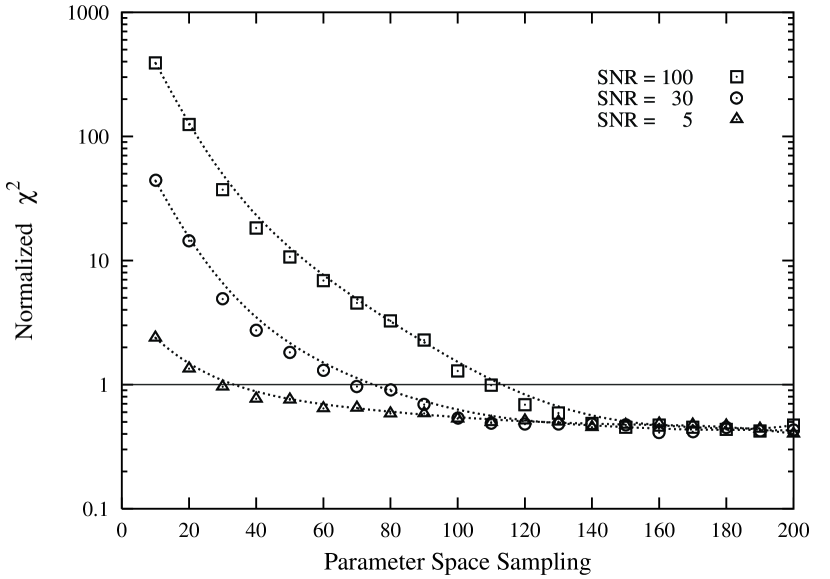
Figure 8: Minimum value of the normalised likelihood term $\chi^{2}/N_{\mathrm{data}}$ that can be reached as the number of basis functions varies and for different signal-to-noise ratios. In abscissa is given the number of samples along $\eta$ and $h$, which is the square root of the number of basis functions used. The number of data measurements were $50\times 50$ and the maximum disk radius was $R_{\mathrm{max}}=7$. The curves are only here to clarify the figure: the simulation results are plotted as symbols.

The best sampling of the phase space of $f$ must be derived considering that two opposite criteria should be balanced: (i) using too few basis functions would bias the solution, (ii) using more basis functions consumes more cpu time. A simple and intuitive way to check that the sampling rate is sufficient is to insure that the minimum likelihood reached without regularisation is much smaller than the target likelihood, i.e. $\lim_{\mu\rightarrow 0}L({\textbf{{f}}})\ll N_{\mathrm{e}}$. Unregularised inversions of noisy data with an increasing number of basis functions and signal-to-noise ratios was therefore performed. In practice, since completely omitting the regularisation leads to a difficult minimisation problem because of a large number of local minima, regularisation was instead relaxed by using a target likelihood somewhat lower than the number of measurements ($N_{\mathrm{e}}\simeq 0.1\times N_{\mathrm{data}}$). The results of these simulations are displayed in Fig. 8. It appears that $\sim 150\times 150$ basis functions are sufficient to avoid the sampling bias. In all the other simulations, $150\times 150$ or $200\times 200$ basis functions are used.

4.2.6 Efficiency: truncation in the measurements

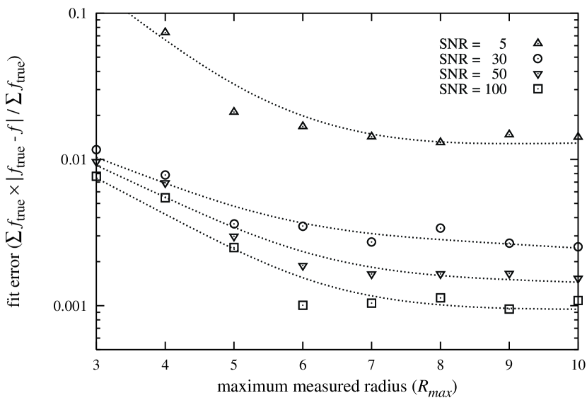
Figure 9: Evolution of the fit error as the data set is truncated in radius for different signal-to-noise ratios (in the simulations the disk outer edge was assumed to be 10; the curves are only here to guide the eye: the results of simulation are plotted as symbols).

The inversion algorithm presented here makes no assumption about completeness of the input data set. Therefore, the recovered solution $f$ can in principle be used to predict missing values in $F_{\phi}$ – in contrast to direct inversion methods which assume that $F_{\phi}$ is known everywhere. Real data will always be truncated at some maximum radius $R\leq{}R_{\mathrm{max}}$. There may also be missing measurements for instance due to dust clouds which hide some parts of the disk, or departure from axial symmetry corresponding to spiral structure. In order to check how extrapolation proceeds, various truncated data were simulated sets and carried the inversion. Figure 9 shows the departure of the recovered distributions from the true one as a function of the outer radius $R_{\mathrm{max}}$ up to which data is measured. This figure also shows that our inversion allows some extrapolation since for all signal-to-noise ratios considered, the error reaches it minimum value as soon as $R_{\mathrm{max}}\geq 7$ (i.e. 4 half mass radii, $R_{e}$, to be compared to the true disk radius which was 10 in our simulations). Note that interpolation is likely to be more reliable than extrapolation; our method should therefore be much less sensitive to data “holes”.

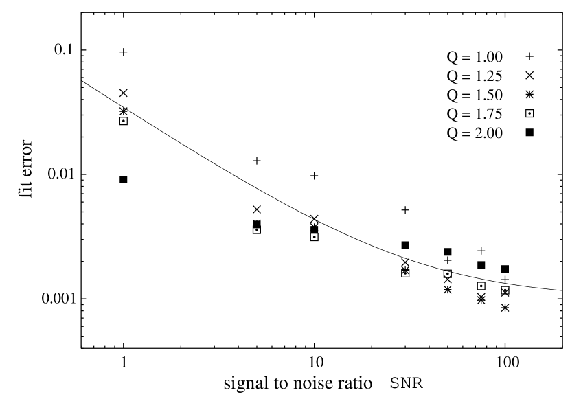
Figure 10: Fit error versus SNR for various Toomre parameters $Q$. The fit error approximatively decreases as: ${\mathrm{error}}\simeq 1.0\times 10^{-3}+3.4\times 10^{-2}/{S\!N\!R}$ (solid line curve).

5 Discussion & Conclusion

This paper presented a series of practical algorithms to obtain the distribution function $f$ from the measured distributions $F_{\phi}(R,v_{\phi})$, compared those to existing algorithms and described in details the best suited to carry efficient inversion of such ill-conditioned problems. It was argued that non-parametric modelisation is best suited to describe the underlying distribution functions when no particular physical model is to be favoured. For these inversions, regularisation is a crucial issue and its weight should be tuned “on the fly” according to the noise level.

The mimimization algorithms brought forward in section 3 are fairly general and could clearly be implemented to minimization problems corresponding to other geometries such as that corresponding to the recovery of distributions for spheroid or elliptical galaxies explored by other authors (e.g. Merritt & Tremblay [Merritt, David Tremblay, Benoit,, 97]). More generally it could be applied to any linear inversion problem where positivity is an issue; this includes image reconstruction, all Abel deprojection arising in astronomy, etc. Applying this algorithm to simulated noisy data, it was found that the criteria of positivity and smoothness alone are sufficiently selective to regularize the inversion problem up to very low signal-to-noise ratios (${S\!N\!R}\sim 5$) as soon as data is available up to 4 $R_{e}$. The inversion method described here is directly applicable to published measurements.

Here the inversion assumed that the HI rotation curve gives access to an analytic (or spline) form for the potential. A more general procedure should provide a simultaneous recovery of the potential, though such a routine would be very CPU intensive since chanching the potential requires to recompute the matrix a. Nevertheless, it would be straightforward to extend the scope of this method to configurations corresponding to an arbitrary slit angle as sketched in the Appendix C, or to data produced by integral field spectroscopy [such as TIGRE or OASIS [Bacon et al., 1995]] where the redundancy in azimuth would lead to higher signal to noise ratios if the disk is still assumed to be flat and axi-symmetric.

Once the distribution function has been characterised, it is possible to study quantitatively all departures from the flat axisymmetric stellar models. Indeed, axisymmetric distribution functions are the building blocks of all sophisticated stability analyses, and a good phase space portrait of the unperturbed configuration is clearly needed in order to asses the stability of a given equilibrium state. Numerical N-body simulations require sets of initial conditions which should reflect the nature of the equilibrium. Linear stability analysis also rely on a detailed knowledge of the underlying distribution[Pichon & Cannon, 1997].

Appendix A Bilinear interpolation

In this non-parametric approach, the distribution $\hat{f}(\eta,h)$ is described by its projection onto a basis of functions. If we choose a basis for which the two variables $\eta$ and $h$ are separable then Eq. (8) becomes:

$$\hat{f}(\eta,h)=\sum_{k}\sum_{l}f_{k,l}\,u_{k}(\eta)\,v_{l}(h)\,,$$ (46)

where $u_{k}(\eta)$ and $v_{l}(h)$ are the new basis functions. This description of $\hat{f}(\eta,h)$ yields:

$$\tilde{F}_{\phi}(R_{i},{v_{\phi}}_{j})=\tilde{F}_{i,j}=\sum_{k}\sum_{l}a_{i,j,k,l}\,f_{k,l}\,,$$ (47)

where $a_{i,j,k,l}$ are coefficients which only depends on $R_{i}$, ${v_{\phi}}_{j}$ and $\psi_{i}$ ($\psi(R)$ in fact):

$$a_{i,j,k,l}=v_{l}(R_{i}\,{v_{\phi}}_{j})\sqrt{-2{{\varepsilon}_{\mathrm{min}}}_{i,j}}\int^{1}_{{\eta_{\mathrm{c}}}_{i,j}}\frac{u_{k}(\eta)}{\sqrt{\eta-{\eta_{\mathrm{c}}}_{i,j}}}\,{{\mathrm{d}}{\eta}}\,.$$ (48)

Bilinear interpolation is implemented in the simulations described in section 4 to evaluate $\hat{f}(\eta,h)$ everywhere. In this case, the weights $f_{k,l}$ are the values of the distribution at the sampling positions $\{(\eta_{k},h_{l});k=1,\dots,K;l=1,\dots,L\}$:

$$f_{k,l}=\hat{f}(\eta_{k},h_{l})\,,$$

and the basis functions are linear splines:

$$u_{k}(\eta) = \left\{\begin{array}[]{ll}1-\left|\frac{\eta-\eta_{k}}{\Delta\!\eta}\right|&\mbox{if $\eta_{k-1}\leq\eta\leq\eta_{k+1}$,}\\ 0&\mbox{otherwise,}\\ \end{array}\right.$$

$$v_{l}(h) = \left\{\begin{array}[]{ll}1-\left|\frac{h-h_{l}}{\Delta\!h}\right|&\mbox{if $h_{l-1}\leq{}h\leq{}h_{l+1}$,}\\ 0&\mbox{otherwise,}\\ \end{array}\right.$$

with $\eta_{k+n}=\eta_{k}+n\,\Delta\!\eta$ and $h_{l+n}=h_{l}+n\,\Delta\!h$. The bilinear interpolation is a particular case of the general non-parametric description. It yields a very sparse matrix a which can significantly speed up matrix multiplications. The coefficients $a_{i,j,k,l}$ can be computed analytically, though since the basis functions are defined piecewise, the integration much be performed piecewise:

$$\int_{\eta_{\mathrm{c}}}^{1}\frac{u_{k}(\eta)}{\sqrt{\eta-{\eta_{\mathrm{c}}}}}\,{{\mathrm{d}}{\eta}}=\left\{\begin{array}[]{ll}\alpha^{\prime\prime}_{k}&\mbox{for $k=1$,}\\ \alpha^{\prime}_{k}+\alpha^{\prime\prime}_{k}&\mbox{for $k=2,\ldots,K-1$,}\\ \alpha^{\prime}_{k}&\mbox{for $k=K$,}\\ \end{array}\right.$$

with:

$$\alpha^{\prime}_{k}=\int_{{\mathrm{max}}\!\{\eta_{k-1},{\eta_{\mathrm{c}}}\!\}}^{{\mathrm{min}}\!\{\eta_{k},1\!\}}\frac{u_{k}(\eta)}{\sqrt{\eta-{\eta_{\mathrm{c}}}}}\,{{\mathrm{d}}{\eta}}\,,$$

$$\phantom{\alpha^{\prime}_{k}}=\!\Biggl{\{}\!\!\!\begin{array}[]{ll}0&\mbox{if $\eta_{k}\!\leq\!{\eta_{\mathrm{c}}}$,}\\ \left[\frac{2\sqrt{\eta-{\eta_{\mathrm{c}}}}}{3\Delta\!\eta}(\eta\!-\!3\eta_{k-1}\!+\!2{\eta_{\mathrm{c}}})\right]_{\eta={{\mathrm{max}}\!\{\eta_{k-1},{\eta_{\mathrm{c}}}\!\}}}^{\eta={{\mathrm{min}}\!\{\eta_{k},1\!\}}}&\mbox{otherwise.}\\ \end{array}$$

and

$$\alpha^{\prime\prime}_{k}=\int_{{\mathrm{max}}\!\{\eta_{k},{\eta_{\mathrm{c}}}\!\}}^{{\mathrm{min}}\!\{\eta_{k+1},1\!\}}\frac{u_{k}(\eta)}{\sqrt{\eta-{\eta_{\mathrm{c}}}}}\,{{\mathrm{d}}{\eta}}\,,$$

$$\phantom{\alpha^{\prime\prime}_{k}}=\!\Biggl{\{}\!\!\!\begin{array}[]{ll}0&\mbox{if $\eta_{k+1}\!\leq\!{\eta_{\mathrm{c}}}$}\\ \left[\frac{2\sqrt{\eta-{\eta_{\mathrm{c}}}}}{3\Delta\!\eta}(3\eta_{k+1}\!-\!\eta\!-\!2{\eta_{\mathrm{c}}})\right]_{\eta={{\mathrm{max}}\!\{\eta_{k},{\eta_{\mathrm{c}}}\!\}}}^{\eta={{\mathrm{min}}\!\{\eta_{k+1},1\!\}}}&\mbox{otherwise.}\\ \end{array}$$

Another useful feature of bilinear interpolation is that the positivity constraint is straightforward to implement:

$$\hat{f}(\eta,h)=\sum_{k,l}f_{k,l}u_{k}(\eta)v_{l}(h)\geq 0;\forall(\eta,h)\quad\Leftrightarrow\quad f_{k,l}\geq 0;\forall(k,l)\,.$$

There is no such simple relation for higher order splines.

Appendix B Specific minimisation methods for MEM

Several non-linear methods have been derived specifically to seek the maximum entropy solution. Let us review those briefly so as to compare them with our method (section 3.2.2). In MEM, assuming that (i) the prior p does not depend on the parameters and that (ii) the Hessian of the likelihood term can be neglected, the Hessian of $Q$ is then purely diagonal:

$$\nabla\!\nabla\!Q_{k,l}\simeq\mu\,\nabla\!\nabla\!R_{k,l}=\frac{\mu\delta_{k,l}}{f_{k}}\,.$$

The direction of minimisation is therefore:

$${\delta\!f_{\mathrm{MEM}}}_{k}=-\frac{f_{k}}{\mu}\,\nabla\!Q_{k}\,.$$ (51)

Skilling & Bryan [Skilling & Bryan, 1984] discussed further refinements to speed up convergence. Cornwell & Evans [Cornwell & Evans, 1984] approximated the Hessian $\nabla\!\nabla\!Q$ by neglecting all non-diagonal elements:

$$\nabla\!\nabla\!Q_{k,l}\simeq\delta_{k,l}\frac{\mu}{f_{k}}+\delta_{k,l}\sum_{i,j}\frac{a_{i,j,k}^{2}}{{\mathrm{Var}}(\tilde{F}_{i,j})}\,,$$

which yields:

$${\delta\!f_{\mathrm{CE}}}_{k}=-\frac{f_{k}\,\nabla\!Q_{k}}{\mu+f_{k}\sum_{i,j}{a_{i,j,k}^{2}}/{{\mathrm{Var}}(\tilde{F}_{i,j})}}\,.$$ (52)

In fact, ${\delta\!f_{\mathrm{CE}}}_{k}$ is equivalent to a steepest descent step in the Levenberg-Marquart method [Press et al., 1988] which is the method of predilection to fit a parametric non-linear model. Extending the Richardson-Lucy method to the maximum penalised likelihood régime, Lucy [Lucy, 1994] suggests:

$${\delta\!f_{\mathrm{Lucy}}}_{k}=-f_{k}\left[\nabla\!Q_{k}-\frac{\sum_{l}f_{l}\nabla\!Q_{l}}{\sum_{l}f_{l}}\right]\,,$$ (53)

which is almost the same as in classical MEM but for the term $\sum_{l}f_{l}\nabla\!Q_{l}/\sum_{l}f_{l}$ which accounts for the constraint that $\sum_{k}f_{k}$ should remain constant. Note that it is sufficient to replace $\nabla\!Q_{k}$ in Eq. (30) by $\nabla\!Q_{k}-\sum_{l}q_{l}\nabla\!Q_{l}/\sum_{l}q_{l}$ to apply a further constraint of normalisation.

With all these non-linear methods, it may be advantageous to also seek the step size which minimises $Q({\textbf{{f}}}+\lambda\delta{\textbf{{f}}})$ [Cornwell & Evans, 1984, Lucy, 1994].

Appendix C General model with arbitrary slit orientation

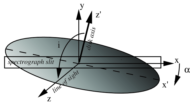
Figure 11: Angular notations

Long slit spectroscopic observations of a galactic disk provide the distribution:

$$F_{\alpha}(R,v_{/\!/})=\int f({\varepsilon},h)\,{{\mathrm{d}}{v_{\perp}}}\,,$$ (54)

where $v_{/\!/}$ and $v_{\perp}$ are the star velocities (at intrinsic radius,$r$ and projected radius $R$) along and perpendicular to the line of sight respectively, that are related to the radial and azimuthal velocities:

$$v_{R}=c_{1}\,v_{/\!/}+c_{2}\,v_{\perp}\,,\quad v_{\phi}=c_{3}\,v_{/\!/}+c_{4}\,v_{\perp}\quad\mbox{and}\quad R=c_{5}\ r\,.$$

Here the $c_{k}$ depend on the angle $\alpha$ between the slit and the major axis of the disk as measured in the plane of the sky and on the inclination $i$ of the disk axis with respect to the line of sight (see Fig. 11). The case where the slit is parallel to the major axis of the disk, i.e. $\alpha=0$, as been examined in the main text. When $\alpha\not=0$, the specific angular momentum $h=r\,v_{\phi}$ can be used as variable of integration:

$$F_{\alpha}(R,v_{/\!/})=\frac{c_{5}}{R\,c_{4}}\int_{-{h_{\mathrm{max}}}}^{{h_{\mathrm{max}}}}f({\varepsilon},h)\,{{\mathrm{d}}{h}}.$$ (55)

where the specific energy and the integration bounds are:

$${\varepsilon} = \frac{1}{2}v_{/\!/}^{2}+\frac{1}{2}\left(\frac{h\,c_{5}}{R\,c_{4}}-\frac{c_{3}}{c_{4}}\,v_{/\!/}\right)^{2}-\psi\left(\frac{R}{c_{5}}\right)\,,$$

$${h_{\mathrm{max}}} = \frac{R}{c_{5}}\left(\frac{c_{3}}{c_{4}}\,v_{/\!/}+\sqrt{2\psi\left(\frac{R}{c_{5}}\right)-v_{/\!/}^{2}}\right)\,.$$

In practice, straightforward trigonometry yields

$$c_{1} = \sin(\beta)/\sin(i)\,,\,\,c_{2}=\cos(\beta)\,,\,\,$$

$$c_{3} = \cos(\beta)/\sin(i)\,,\,\,c_{4}=\sin(\beta)\,,\,\,$$

$$c_{5}=\sqrt{\cos^{2}(\beta)+\sin^{2}(\beta)\sin^{2}(i)}\,,$$

where $\beta$ is the angle of the slit as measured in the plane of the disk which obeys

$$\tan(\beta) = \tan(\alpha)/\sin(i)\,.$$

References

- [Bacon et al., 1995] Bacon, R. et al. 1995, Astron. Astrophys. Suppl. Ser. 113, 347.
- [Cornwell & Evans, 1984] Cornwell, T.J. & Evans, K.F., 1984, AA 143, 77.
- [Dejonghe, 1993] Dejonghe, H. 1993, in Galactic Bulges, IAU Symp. No. 153, ed. H. Dejonghe & H. J. Habing (Kluwer: Dordrecht), 73.
- [Dejonghe et al., 1996] Dejonghe, H., De Bruyne, V., Vauterin, P. and Zeilinger, W. W., 1996, The internal dynamics of very flattened normal galaxies. Stellar distribution functions for NGC 4697. , AAp, feb, 306-363.
- [Dehnen, 1995] Dehnen, W. 1995, MNRAS, 274, 919.
- [Emsellem et al., 1994] Emsellem, E., Monnet, G., & Bacon, R., 1994, AAp, 285, 723.
- [Gebhardt, Karl; Richstone, Douglas; Ajhar, Edward a.; Lauer, Tod r.; Byun, Yong-Ik; Kormendy, John; Dressler, Alan; Faber, S. m.; Grillmair, Carl; Tremaine, Scott, 1996] Astronomical Journal v.112, p.105
- [Gull, 1989] Gull, F., 1989, in: Maximum Entropy and Bayesian Methods (J. Skilling editor, Kluwer Academic publisher), p. 53.
- [Horne, 1985] Horne, K., 1985, MNRAS 213, 129.
- [Kuijken, 1995] Kuijken, K. 1995, ApJ, 446, 194.
- [Lane, 1992] Lane, R. G. 1992, J. Opt. Soc. Am. A 9, 1508–1514.
- [Lucy, 1994] Lucy, L.B., 1994, AA 289, 983.
- [Merrifield, 1991] Merrifield, M. R. 1991, AJ, 102, 1335.
- [Merritt, David,, 1997] Merritt, David,1997, Astronomical Journal,114, 228–237.
- [Merritt, David,, 1996] Merritt, David,1996, Astronomical Journal, 112 , 1085.
- [Merritt, David Tremblay, Benoit,, 97] Merritt, David and Tremblay, Benoit”,1993, Astronomical Journal, 106, 2229–2242.
- [Merritt & Gebhardt, 1994] Merritt, D. & Gebhardt, K. 1994, in Clusters of Galaxies, Proceedings of the XXIXth Rencontre de Moriond, ed. F. Durret, A. Mazure & J. Tran Thanh Van (Editions Frontiere: Singapore), p. 11.
- [Merritt & Tremblay, 1994] Merritt, D. & Tremblay, B. 1994, “Nonparametric estimation of density profiles”, The Astronomical Journal, vol. 108, no. 2, p. 514+
- [Narayan & Nityananda, 1986] Narayan, R., and Nityananda, R., 1986, Ann. Rev. Astron. Astrophys. 24, 127.
- [Press et al., 1988] Numerical Recipes (Press, et. al. Cambridge University Press 1988).
- [Pichon & Cannon, 1997] Pichon, C. & Cannon, R. 1997, “Numerical stability analysis of flat and round disks”, Mont. Not. R. Astron. Soc. 291 616-632.
- [Pichon & Lynden-Bell, 1996] Pichon, C. and Lynden-Bell, D. 1996, “The equilibria of flat and round disks”, 1996, MNRAS 282 (4), 1143-1158.
- [Qian, 1995] Qian, E. E., de Zeeuw, P. T., van der Marel, R. P. & Hunter, C. 1995, MNRAS, 274, 602.
- [Skilling & Bryan, 1984] Skilling, J., & Bryan, R. K., 1984, MNRAS 211, 111–124 [also denoted SB in this article].
- [Skilling, 1989] Skilling, J., 1989, in: Maximum Entropy and Bayesian Methods (J. Skilling editor, Kluwer Academic publisher), p. 45.
- [Thiébaut & Conan, 1995] Thiébaut, E. and Conan, J.-M. 1995, “Strict a priori constraints for maximum likelihood blind deconvolution”, J. Opt. Soc. Am. A 12, 485–492.
- [Thompson & Craig, 1992] Thompson, A.M. & Craig, I.J.D., 1992, AA 262, 359.
- [Titterington, 1985] Titterington, D.M., 1985, AA 144, 381.
- [Toomre, 1964] Toomre, A. 1964, “On the Gravitational Stability of a Disc of Stars.” Astrophysical Journal 139, 1217-1238.
- [Wahba & Wendelberger, 1979] Wahba, G. & Wendelberger, J. 1979, “Some New Mathematical Methods for Variational Objective Analysis Using Splines and Cross Validation.” Monthly Weather Review 108, 1122-1143.
- [Wahba , 1990] Wahba, G., 1990, “Spline models for Observational Data.” CBMS-NSF Regional conference series in applied mathematics, Society for industrial and applied mathematics, Philadelphia.