The Keplerian map for the restricted three-body problem as a model of comet evolution

Abstract

We examine the evolution of highly eccentric, planet-crossing orbits in the restricted three-body problem (Sun, planet, comet). We construct a simple Keplerian map in which the comet energy changes instantaneously at perihelion, by an amount depending only on the azimuthal angle between the planet and the comet at the time of perihelion passage. This approximate but very fast mapping allow us to explore the evolution of large ensembles of long-period comets. We compare our results on comet evolution with those given by the diffusion approximation and by direct integration of comet orbits. We find that at long times the number of surviving comets is determined by resonance sticking rather than a random walk.

1 Introduction

The orbits of small bodies in the outer solar system, such as planetesimals or comets, evolve through gravitational interactions with the giant planets. This process determines the structure of the Oort Cloud, the rate of depletion of the Kuiper belt, the total population and spatial distribution of the Centaurs, and the dynamical properties of observed comets. Understanding the nature of planet-induced orbital evolution is therefore important for a wide range of solar system problems.

A particularly important issue is the evolution of highly eccentric orbits whose perihelia penetrate the region of the outer planets (e.g. long-period comets). In this case the evolution can be treated approximately as a one-dimensional random walk in energy; the energy change per perihelion passage is assumed to be a Gaussian random variable and the rms energy change is assumed to be small compared to the typical orbital energy. This “diffusion approximation” was introduced by Oort (1950) and has been employed by many authors, including Whipple (1962), Weissman (1978), Yabushita (1980), Bailey (1984), and Duncan et al. (1987). A closely related approach is to treat the evolution as a random walk; thus the energy change at perihelion is assumed to be a random variable but it is not assumed to be small compared to the orbital energy (Kendall 1961, Arnold 1965, Öpik 1976, Everhart 1977, 1979, Yabushita 1979, Froeschlé and Rickman 1980). The diffusion or random-walk approximation provides considerable insight into the evolution of comet orbits, but neglects potentially important effects such as secular evolution, resonances, etc.

Direct numerical integrations provide the most accurate way to analyze orbital evolution. The evolution of long-period comets under the gravitational influence of the giant planets has been examined by Wiegert and Tremaine (1998), and extensive integrations of short-period comets and Kuiper-belt objects have been carried out by Holman and Wisdom (1992) and by Duncan and Levison (1997). Numerical integrations require more work, which can be prohibitive, and may yield less insight than simpler methods. Thus it remains worthwhile to investigate approximate models for planet-induced orbital evolution.

Clearly the random-walk approximation fails for orbits with semimajor axes comparable to those of the outer planets, since in this case the energy changes are correlated at successive perihelion passages. A simple approach that illuminates this transition is to replace the random energy change at perihelion in the random-walk approximation with an energy change that depends on the azimuthal phase of the planet at perihelion passage; thus the energy at successive perihelion passages is determined by a deterministic twist map of the form

$$E_{n+1} = E_{n}+F(\psi_{n}),$$

$$\psi_{n+1} = \psi_{n}+\Omega_{p}P(E_{n+1}),$$ (1)

where $E$ is the specific energy, $\Omega_{p}$ is the planet’s angular speed, $P(E)\propto|E|^{-3/2}$ is the comet’s orbital period, $\psi$ is the azimuthal angle between the planet and the comet perihelion at the time of perihelion passage, and $F$ represents the energy changes caused by the planet at perihelion passage. This map was examined by Petrosky (1986) using a simple—but unrealistic—sinusoidal form for $F$; Petrosky called (1) the Keplerian map, a term that we shall also adopt. Sagdeev and Zaslavsky (1987) derived the map independently, evaluating $F$ in the simple but uninteresting limit that the perihelion distance was much larger than the planet’s semimajor axis (they also neglected the indirect term in the gravitational potential from the planet). Chirikov and Vecheslavov (1989) used the map to examine the long-term evolution of Halley’s comet.

The aim of this paper is to provide a fairly rigorous derivation of the Keplerian map, to discuss its generalizations, to provide better approximations for the “kick function” $F$ than have been available so far, and to compare the predictions of the map both to numerical integrations and the diffusion approximation, to clarify the strengths and weaknesses of each approach. One of our principal results is that the number of comets that survive for many orbits is much larger than predicted by the diffusion or random-walk approximation, a result that we ascribe to “resonance sticking”.

Mostly we shall examine the motion of comets in a planetary system containing the Sun and a single planet of mass $M_{p}$ on a circular orbit. Without loss of generality we may choose the period and the semimajor axis of the planet to be unity. With this choice of units the planet’s mean motion $\Omega_{p}=2\pi$, $G(M_{\odot}+M_{p})=4\pi^{2}$, $P(E)=2^{3/2}\pi^{3}/(|E|^{3/2})$ is the comet’s orbital period, and the specific energy of the planet $E_{p}=-2\pi^{2}$. We also write $m_{p}\equiv M_{p}/M_{\odot}$.

1.1 The diffusion approximation

In this approximation the evolution of the comet orbit is treated as a one-dimensional random walk in energy, the mean-square energy change per perihelion passage $D$ is assumed to be independent of energy and $D^{1/2}$ is assumed to be small compared to the typical comet energy $E$. Then the number of comets bound to the solar system at time $t$ with energy in the range $[E,E+dE]$ is $n(E,t)dE$, where

$${\partial n\over\partial t}={\textstyle{1\over 2}}D{\partial^{2}\over{\partial E^{2}}}\left[n\over P(E)\right].$$ (2)

A more convenient form is

$${\partial n\over\partial t}=m_{p}^{2}D_{0}{\partial^{2}\over{\partial E^{2}}}\left[{(-E)}^{3/2}n\right],$$ (3)

where $D_{0}$ is independent of the planetary mass,

$$m_{p}^{2}D_{0}={1\over 2^{5/2}\pi^{3}}D={1\over 2^{5/2}\pi^{3}}\langle(\Delta E)^{2}\rangle,$$ (4)

and the average $\langle\cdot\rangle$ is taken over the phase of the planetary orbit at a single perihelion passage.

The solution to equation (2) depends on the boundary conditions. The simplest assumption is that all comets with positive energy escape, so $n=0$ for $E\geq 0$. In this case the Green’s function corresponding to the initial distribution $n(E,t=0)=\delta(E-E_{0})$, $E_{0}<0$, is (Yabushita 1980)

$$n(E,t)=\frac{2|E_{0}|^{1/2}}{m_{p}^{2}D_{0}t|E|}\exp\left(-\frac{4}{m_{p}^{2}D_{0}t}\left[|E_{0}|^{1/2}+|E|^{1/2}\right]\right)I_{2}\left(\frac{8}{m_{p}^{2}D_{0}t}(EE_{0})^{1/4}\right),$$ (5)

where $I_{2}$ is a modified Bessel function. The total number of surviving comets after time $t$ is given by the depletion function

$$N(t)=\int_{0}^{\infty}n(E,t)dE=\gamma\left[2,\;4{|E_{0}|}^{1/2}/(m_{p}^{2}D_{0}t)\right],$$ (6)

where $\gamma$ is an incomplete gamma function. At large times $N(t)\to 8|E_{0}|\left/{(m_{p}^{2}D_{0}t)}^{2}\right.$. Note that equations (5) and (6) are normalized so that the initial number of comets $N(t=0)=1$.

A more accurate approximation is that comets are lost if either $E\geq 0$ or $E\leq E_{min}$; the absorbing boundary at $E_{min}$ arises because comets in tightly bound orbits may collide with the Sun, evaporate, or evolve much more quickly under the influence of more massive planets. In this case it is straightforward to solve equation (3) numerically to find the depletion function.

2 Mapping method

We examine the orbit of a test particle (the comet) moving in the combined gravitational field of the Sun and a single planet on a circular orbit (the restricted three-body problem). We restrict our attention to comets with small inclinations, since we are mostly interested in scattering of comets in the protoplanetary disk. Thus the comet’s phase-space position is described by its semimajor axis $a$, eccentricity $e$, argument of perihelion $\varpi$, and mean anomaly $\ell$. Alternatively we may use canonical elements. The simplest of these are the coordinate-momentum pairs $(\ell,\;K=[GM_{\odot}a]^{1/2})$ and $(\varpi,L)$, where $L=[GM_{\odot}a(1-e^{2})]^{1/2}$ is the specific angular momentum. The azimuth of the planet at time $t$ may be written $\phi_{p}(t)=\Omega_{p}t+\phi_{0}=2\pi t+\phi_{0}$.

The equations of motion are described by a Hamiltonian

$$H(K,L,\ell,\varpi,t)=-{8\pi^{4}\over K^{2}}+m_{p}H_{1}(K,L,\ell,\varpi,t).$$ (7)

For our purposes it is more convenient to use mean anomaly instead of time as the independent variable. Then the equations of motion are still Hamiltonian if we use $(\varpi,L)$ and $(t,-E)$ as canonical coordinates and $-K(L,E,\varpi,t,\ell)$ as the Hamiltonian, where $K$ is defined implicitly by $E=H(K,L,\ell,\varpi,t)$ and $E$ is the energy. In other words

$${dL\over d\ell}={\partial K\over\partial\varpi},\quad{dE\over d\ell}=-{\partial K\over\partial t},\quad{d\varpi\over d\ell}=-{\partial K\over\partial L},\quad{dt\over d\ell}={\partial K\over\partial E}.$$ (8)

We shall now focus on long-period comets. These spend most of their time at distances much greater than the planet’s semimajor axis, where they travel on near-Keplerian orbits around the Sun-planet barycenter. Changes in the comet’s energy and other orbital elements are localized near perihelion, where its interactions with the planet are strongest. Therefore it makes sense to assume that the encounter with the planet lasts for only a short time near perihelion ($\ell=0$). Furthermore since $m_{p}\ll 1$ the perturbation from the planet is weak. Thus we may write the negative of the Hamiltonian as

$$K(L,E,\varpi,t,\ell)={4\pi^{2}\over(-2E)^{1/2}}+m_{p}\kappa(L,E,\varpi,t)\delta_{2\pi}(\ell)+\hbox{O}(m_{p}^{2}),$$ (9)

where $\delta_{2\pi}(x)=\sum_{n}\delta(x-2\pi n)$ is the periodic Dirac delta-function and $\kappa=-4\pi^{2}(-2E)^{-3/2}\int H_{1}d\ell$. Furthermore, $\kappa$ can only depend on the time through the planet azimuth $\phi_{p}(t)$ and can only depend on the azimuthal angles $\phi_{p}(t)$ and $\varpi$ through the combination $\psi=\phi_{p}(t)-\varpi=2\pi t+\phi_{0}-\varpi$. Thus we may write

$$K(L,E,\varpi,t,\ell)={4\pi^{2}\over(-2E)^{1/2}}+m_{p}\kappa(L,E,2\pi t+\phi_{0}-\varpi)\delta_{2\pi}(\ell).$$ (10)

Equations (8) and (10) imply that the Jacobi constant

$$J\equiv E-2\pi L$$ (11)

is conserved, a property that we inherit from the restricted three-body problem. Note also that $\kappa$ is conserved as the trajectory crosses $\ell=0$.

To proceed further we shall adopt a simple functional form for $\kappa(L,E,\psi)$ that (we hope) captures the most important physics of the interaction. A natural first approximation is that $\kappa$ is independent of $E$ and $L$, so that $\kappa=\kappa(\psi)$ (we discuss more general forms in §4). The assumption that $\kappa$ is independent of energy is reasonable for long-period comets, which all have near-parabolic orbits in the vicinity of the planets. The assumption that $\kappa$ is independent of angular momentum is less natural since the interaction of a long-period comet with the planets depends strongly on its perihelion distance; however, the same assumption is made in the diffusion approximation (eq. 3), and conservation of the Jacobi constant (eq. 11) ensures that variations in $L$ are small so long as the comets remain long-period (i.e. $|E|\ll 1$).

Hamilton’s equations (8) can now be integrated from $\ell=2\pi n-0$ to $2\pi(n+1)-0$:

$$\varpi = \mbox{const},$$

$$E_{n+1} = E_{n}+m_{p}f(\psi_{n}),$$

$$L_{n+1} = L_{n}+{m_{p}\over 2\pi}f(\psi_{n}),$$

$$t_{n+1} = t_{n}+2^{3/2}\pi^{3}(-E_{n+1})^{-3/2},$$

$$\psi_{n+1} = \psi_{n}+2\pi(t_{n+1}-t_{n}),$$ (12)

where the “kick function” $f(\psi)=-2\pi d\kappa(\psi)/d\psi$ is independent of planet mass, and the map we have derived is essentially the Keplerian map (1).

Thus we have arrived at a symplectic mapping in two dimensions ($\psi,E$), which depends on the planet mass and the kick function. The angular momentum $L$ is determined by the energy and the Jacobi constant $J$ (eq. 11). The derivation of the map was motivated by long-period comets, whose orbital period is much longer than the planet orbital period ($P(E)/P(E_{p})=(2\pi^{2}/|E|)^{3/2}\gg 1$); however, it should also provide a fair representation of the behaviour of orbits with shorter periods, $|E|/(2\pi^{2})\sim 1$.

Mappings such as (12) can have trajectories of two kinds, regular and stochastic. The energy of regular orbits will vary only over a limited range, whereas stochastic orbits can wander over the entire stochastic region, and in particular they can reach escape energy ($E\geq 0$), which corresponds to loss of a comet from the solar system. The comet is also lost if $L\leq 0$, which corresponds to collision with the Sun and occurs if $E\leq J$.

2.1 The kick function

To determine the kick function $f(\psi)$ we numerically integrated the orbits of a set of comets on initially parabolic orbits through a single perihelion passage. The comets shared a common perihelion distance $q$ and were distributed uniformly random in argument of perihelion and longitude of ascending node. The inclinations were chosen at random from a narrow Gaussian distribution with zero mean and dispersion $0.1$ radians. Then we calculated the energy change $\Delta E=E_{final}-E_{initial}$ in the barycentric frame and averaged $\Delta E$ over all comets with a given value of $\psi$, which is the azimuthal angle between the comet and planet at the instant of perihelion passage. The kick function is the average energy change normalized by the planet mass, $f(\psi)=\langle\Delta E\rangle/m_{p}$. Figure 1(a) shows a scatter plot of the normalized energy change $\Delta E(\psi)/m_{p}$ versus $\psi$ for 30,000 passages with perihelion distance $q=0.5$. The Figure also shows the corresponding kick function $\langle\Delta E\rangle/m_{p}$, averaged over $2000$ comets at each of $600$ values of $\psi$. As we should expect, the kick function is approximately odd, $f(-\psi)=-f(\psi)$. The sharp changes in the kick function correspond to close encounters with the planet, which occur at

$$\psi=\pm\left[\arccos(2q-1)-2^{1/2}(1-q)^{1/2}(2q+1)/3\right].$$ (13)

Kick functions for different perihelion distances are shown in Figure 1(b). (Everhart (1968) made an impressive early effort to obtain an empirical fit to the distribution of energy changes caused by planetary perturbations; however, his results are averaged over $\psi$ and thus are not useful for our purposes.)

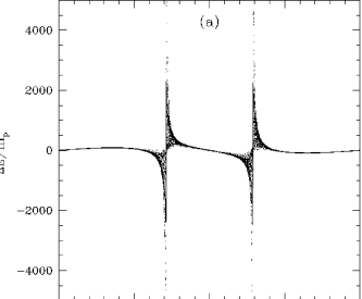
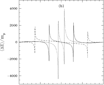
Figure 1: (a) The points show the energy change $\Delta E(\psi)/m_{p}$ for a sample of initially parabolic comets with perihelion distance $q=0.5$. The solid line is the kick function $\langle\Delta E(\psi)\rangle/m_{p}=f(\psi)$ for this perihelion distance. (b) Kick functions for perihelion distances $q=0.1$ (dashed line), $q=0.5$ (solid line), and $q=0.9$ (dot line). It is an artifact of the plotting program that the curves are not precisely odd in $\psi$ near the spikes.

In our mapping (12) we represent $f(\psi)$ by a continuous interpolation function

$$F(\psi)=-F(-\psi)=\left\{\begin{array}[]{ll}{|\psi-\psi_{0}|}^{-1/2}\sum\limits_{n=1}^{4}C_{n}^{(-)}{(\psi+\pi)}^{n}&-\pi\leq\psi\leq\psi_{-},\\ C_{1}\psi+C_{0}&\psi_{-}<\psi<\psi_{+},\\ {|\psi-\psi_{0}|}^{-1/2}\sum\limits_{n=1}^{4}C_{n}^{(+)}\psi^{n}&\psi_{+}\leq\psi\leq 0,\\ \end{array}\right.$$

where we have divided the interval $[-\pi,0]$ in three parts $[-\pi,\psi_{-}]$, $(\psi_{-},\psi_{+})$, $[\psi_{+},0]$ and define $\psi_{-}$, $\psi_{+}$, and $\psi_{0}$ by

$$f(\psi_{-})=\min\limits_{\psi\in[-\pi,0]}f(\psi),\qquad f(\psi_{+})=\max\limits_{\psi\in[-\pi,0]}f(\psi),\qquad\psi_{0}=(\psi_{-}+\psi_{+})/2.$$ (14)

Of course the function $F(\psi)$ has the same odd symmetry as $f(\psi)$. Note that only 10 of the 12 coefficients are independent, because of the continuity constraint at $\psi_{-}$ and $\psi_{+}$.

The coefficients of the interpolation function $F(\psi)$ are given in Table 1, along with the diffusion coefficient $D_{0}$ defined by equation (4) for initially parabolic orbits with the same inclination distribution.

$q$	$0.1$	$0.3$	$0.5$	$0.7$	$0.9$
$\psi_{-}/\pi$	$-6.26\times 10^{-1}$	$-4.33\times 10^{-1}$	$-2.89\times 10^{-1}$	$-1.73\times 10^{-1}$	$-7.33\times 10^{-2}$
$\psi_{+}/\pi$	$-6.23\times 10^{-1}$	$-4.29\times 10^{-1}$	$-2.86\times 10^{-1}$	$-1.69\times 10^{-1}$	$-7.00\times 10^{-2}$
$C_{1}^{(-)}$	$6.56\times 10^{1}$	$1.47\times 10^{2}$	$1.82\times 10^{2}$	$1.77\times 10^{2}$	$1.50\times 10^{2}$
$C_{2}^{(-)}$	$7.26$	$-4.08$	$-6.22\times 10^{1}$	$-6.83\times 10^{1}$	$-5.37\times 10^{1}$
$C_{3}^{(-)}$	$-1.76\times 10^{2}$	$-9.64\times 10^{1}$	$-2.42\times 10^{1}$	$-9.93$	$-1.07\times 10^{1}$
$C_{4}^{(-)}$	$5.56\times 10^{1}$	$1.76\times 10^{1}$	$2.01\times 10^{-1}$	$-1.15$	$-2.35\times 10^{-1}$
$C_{1}^{(+)}$	$-2.40\times 10^{2}$	$-2.14\times 10^{2}$	$-3.41\times 10^{2}$	$-6.48\times 10^{2}$	$-2.45\times 10^{3}$
$C_{2}^{(+)}$	$-6.84\times 10^{1}$	$8.83\times 10^{1}$	$-6.60\times 10^{2}$	$-2.94\times 10^{3}$	$-2.83\times 10^{4}$
$C_{3}^{(+)}$	$3.06\times 10^{1}$	$3.12\times 10^{2}$	$-1.26\times 10^{3}$	$-1.08\times 10^{4}$	$-2.39\times 10^{5}$
$C_{4}^{(+)}$	$1.04\times 10^{1}$	$1.62\times 10^{2}$	$-8.11\times 10^{2}$	$-1.22\times 10^{4}$	$-6.52\times 10^{5}$
$C_{0}$	$5.83\times 10^{5}$	$6.05\times 10^{5}$	$3.91\times 10^{5}$	$2.82\times 10^{5}$	$1.44\times 10^{5}$
$C_{1}$	$2.96\times 10^{5}$	$4.45\times 10^{5}$	$4.32\times 10^{5}$	$5.24\times 10^{5}$	$6.46\times 10^{5}$
$D_{0}$	$3.9\times 10^{2}$	$5.0\times 10^{2}$	$7.7\times 10^{2}$	$1.0\times 10^{3}$	$1.7\times 10^{3}$

Table 1: The coefficients of the interpolation function $F(\psi)$ and diffusion coefficients (eq. 4) for different perihelion distances.

3 Results

We examine a map with planet mass $m_{p}=5.24\times 10^{-5}$, which corresponds to the mass of Neptune, using the kick function for perihelion distance $q=0.5$ (solid line in Figure 1(b)).

Figure 2(a) illustrates the behavior of the map. The vertical axis is $E/2\pi^{2}$ (the normalization is chosen so that the energy of an orbit with the planet’s semimajor axis is unity), the horizontal axis is $\psi/\pi$, and each point corresponds to one iteration of the map (one perihelion passage). The initial energy and azimuth of the orbits plotted are distributed uniformly random in the range $-2\leq E/2\pi^{2}<0$ and $-\pi\leq\psi<\pi$. The Figure shows the evolution of $100$ comets over a time interval $300$ (recall that the period of the planet orbit is unity). Figure 2(c) shows a magnified view of a smaller energy range, $-1.50\leq E/2\pi^{2}<-1.28$.

Figures 2(b) and 2(d) are the same as Figures 2(a) and 2(c) except that the evolution of the comet orbits is determined by direct integration of the restricted three-body problem. The similarity of the corresponding plots suggests that the map captures most of the relevant dynamics in the restricted three-body problem.

The figures exhibit two main classes of orbit: (i) isolated islands consisting of regular orbits; (ii) a single connected stochastic orbit (the “stochastic sea”). The regular orbits are in resonance with the planetary orbital period. The future evolution of any point in the stochastic sea always terminates with escape ($E>0$) or collision with the Sun ($L\leq 0$). The lower limit of the stochastic sea is at $E=J=E_{init}-2\pi L_{init}$. As the energy approaches escape the fraction of phase space occupied by the stochastic sea grows. Notice that there are no KAM surfaces that extend across all values of the azimuthal angle $\psi$; the reason is that orbits that suffer close encounters with the planet (eq. 13) are always stochastic. Thus stochastic orbits can escape from any energy range. Many of these features are reminiscent of the Fermi map with a non-differentiable forcing function (Lichtenberg and Lieberman 1992).

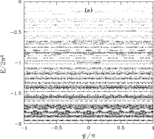
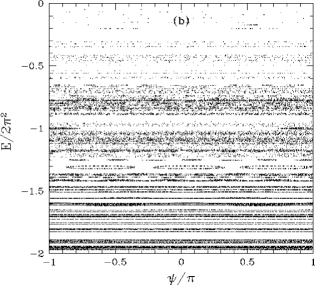
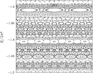
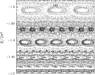
Figure 2: (a) and (c) The perihelion passages of $100$ comets over $300$ planetary orbital periods (“Neptune years”), as determined from the map (12) with perihelion distance $q=0.5$. The comets are initially uniformly distributed in energy and azimuth and the planet mass is $m_{p}=5.24\times 10^{-5}$. (b) and (d) The same as figures (a) and (c), computed by direct numerical integration of the comet orbits.

To explore the evolution of planet-crossing comets over much longer times we have used the map to follow $150,000$ comets with initial energy $E/2\pi^{2}=-0.242$ (corresponding to semimajor axis $4.13$ in units of the planetary semimajor axis) and initial azimuth $\psi$ distributed uniformly random in $[0,2\pi)$. The initial semimajor axis was chosen so that all of the comets were in the stochastic sea and thus can escape. The comets are lost if they reach $E=0$ (escape) or $E/2\pi^{2}=-2.181$ (collision with the Sun, as determined from (11)). We followed the comets for $2.7\times 10^{7}$ time units, which corresponds to the age of the solar system, 4.5 Gyr, if the planet has Neptune’s orbital period. After this time $3.7\%$ of the comets survived. Of the comets that are lost, $96.9\%$ escape and the remainder collide with the Sun. To show the phase portrait of the survivors, we plot every tenth perihelion passage for a time interval of $1000$ Neptune years (Figure 3a). To magnify the detail, we also plot all of the perihelion passages in the interval $-1.50\leq E/2\pi^{2}\leq-1.28$ (Figure 3b).

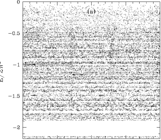
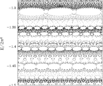
Figure 3: The final phase portrait of $150,000$ comets, after 4.5 Gyr. The planet has Neptune’s mass and orbital period, and the comets initially lie in the stochastic sea, at $E/2\pi^{2}=-0.242$ (semimajor axis $4.13$ in Neptune units). (a) Every tenth perihelion passage of all surviving comets, over an interval of 1000 Neptune years. The mapping structure for $E/2\pi^{2}\lower 2.15277pt\hbox{$\;\buildrel<\over{\sim}\;$}-1.8$ is unreliable since very few comets penetrate to this region (for example, only 3% of the comets are lost through collision with the Sun at $E/2\pi^{2}=-2.181$; all the rest are lost by escape to $E\geq 0$). (b) A magnified view showing all perihelion passages in the interval $-1.50\leq E/2\pi^{2}\leq-1.28$.

It is worthwhile to compare Figures 2(c) and 3(b). The most striking difference is that the islands of regular orbits are empty in 3(b); this of course is because the comets that are shown in 3(b) had initial conditions in the stochastic sea, whereas those in 2(c) were chosen randomly. A more interesting difference is that many of the points in Figure 3(b) are concentrated near the shores of the resonant islands (this is especially noticeable near $E/2\pi^{2}\simeq-1.30$, $-1.41$, $-1.43$ and $-1.49$). This is the well-known phenomenon of resonance sticking: stochastic orbits can be trapped for extended periods in the forest of tiny resonant islands near the shore of the stochastic sea (e.g. Karney 1983, Meiss 1992). We explore this phenomenon further at the end of this section.

To examine the energy distribution of the surviving comets we divided the sample of 150,000 comets into two equal parts. In Figure 4(a) and 4(b) we plot the energy distribution of the surviving comets from each sub-sample after 4.5 Gyr; in particular we plot the normalized distribution of the number of perihelion passages per unit energy interval per unit time, i.e. the function

$$\mu(E,t)=\frac{n(E,t)/P(E)}{\int\limits^{\infty}_{0}n(E,t)/P(E)\,dE}$$ (15)

(see definitions in §1.1). We see that the curves in the two panels have different shapes, which shows that most or all of the fine structure is statistical noise.

Figure 4: The energy distribution of the surviving comets from Figure 3, divided into two equal sub-samples. The energy distribution has been averaged over $10^{5}$ Neptune years to smooth out short-term fluctuations. The spikes are generally not common to the two plots and hence represent statistical noise.

Figures 5(a) and (b) show the depletion function $N(t)$ as a function of time for several different initial energies. Each curve is based on an initial sample of $20,000$ comets. The survival fraction at large times in these plots is unrealistic, as it consists almost entirely of comets that have been kicked into near-escape orbits of very long period (in practice these comets would be removed by tidal forces). The expected asymptotic behavior as $t\to\infty$ is easy to derive heuristically. Let us imagine giving a set of bound comets a broad distribution of energy kicks at $t=0$. Since the distribution of kicks is smooth, the number density of comets as a function of energy is flat near $E=0$, $n(E)dE=\hbox{const}\times dE$. The distribution of orbital periods is then $n(P)dP=n(E)|dE/dP|dP=\hbox{const}\times P^{-5/3}dP$. These comets remain bound until their second perihelion passage, after which they will normally be ejected within a relatively short time. Thus the expected asymptotic shape is

$$N(t)\propto\int\limits_{t}^{\infty}n(P)\,dP\propto t^{-2/3}.$$ (16)

This power law is shown by an arrow on Figure 5(b) and accurately reproduces the behavior of the map.

Figure 5: The logarithm of the fraction of surviving comets in the map (12) as a function of (a) time and (b) log of the time. Each sample initially contained $20,000$ comets uniformly distributed in azimuth, with initial energies $E/2\pi^{2}=-0.985$, $E/2\pi^{2}=-0.490$, $E/2\pi^{2}=-0.242$ and $E/2\pi^{2}=-0.03$. The initial energies are chosen so that all comets lie in the stochastic sea. The slope of the asymptotic law (16) is shown by an arrow.

A more realistic map can be obtained by choosing a slightly negative escape energy, to crudely represent the effects of Galactic tidal forces (e.g. Heisler and Tremaine 1986). In Figures 6(a) and (b) we plot $N(t)$ as determined by mapping 500,000 comets with initial energy $E/2\pi^{2}=-0.242$ and random initial phases. The two solid lines correspond to two different choices for the escape energy, $E_{esc}/2\pi^{2}=0$ and $-0.03$; the latter corresponds to the more realistic case where a comet escapes from the influence of the giant planets when it reaches a semimajor axis $a\sim 1000\mbox{AU}$ where galactic tides and passing stars begin to have significant effects (Duncan, Quinn and Tremaine 1987). When the escape energy is non-zero $N(t)$ decays approximately exponentially [Figure 6(a)] until $t_{s}\sim 5\times 10^{7}$ and thereafter as $t^{-k}$, $k\approx 1.3$ [Figure 6[b]). We interpret this late-time behaviour as the result of resonance sticking.

We may also compare the depletion function in the map to the predictions of the diffusion approximation (eq. 3). The dotted line shows the analytic prediction from equation (6), using the diffusion coefficient $D_{0}$ from Table 1. As we indicated in §1.1, a more accurate approximation is that comets are lost either when $E\geq 0$ (escape) or $E/2\pi^{2}<J/2\pi^{2}=-2.181$ (collision with the Sun). We have also solved equation (3) numerically with these boundary conditions to provide a second prediction of $N(t)$ (dashed line). For reference, we show by solid arrows on Figure 6(b) a power-law depletion law $N(t)\propto t^{-k}$ with $k=1.3$, $k=\frac{2}{3}$ as predicted by equation (16), and $k=2$ as predicted by the diffusion approximation with $E_{min}\to-\infty$ (eq. 6).

Figure 6: The solid lines show the logarithm of the fraction of surviving comets in the map (12) as a function of time (a) and logarithm of time (b). The sample initially contained 500,000 comets with energy $E/2\pi^{2}=-0.242$; these were followed for two values of the escape energy, $E_{esc}/2\pi^{2}=0$ and $E_{esc}/2\pi^{2}=-0.03$. We also plotted two predictions from the diffusion approximation of §1.1. The dotted line is for a single absorbing boundary at $E=0$ (escape) and the dashed line is for two absorbing boundaries at $E=0$ (escape) and $E/2\pi^{2}=J/2\pi^{2}=-2.181$. The asymptotic falloffs $N(t)\propto t^{-2/3}$, $N(t)\propto t^{-2}$ and $N(t)\propto t^{-1.3}$ are shown by arrows.

We close this section by exploring the phenomenon of resonance sticking in more detail. To do so, we map $5\times 10^{6}$ comets with initial energy $E/2\pi^{2}=-0.49$, and consider that a comet is lost anytime it reaches the nearby boundaries $E_{min}/2\pi^{2}=-0.59$, $E_{max}/2\pi^{2}=-0.39$ (focusing on a smaller energy interval provides a more sensitive probe of sticking, since the diffusion time is reduced for fixed diffusion coefficient). The resulting depletion functions for the mapping (eq. 12) and the diffusion approximation (eq. 3) are shown in Figure 7 by solid and dashed lines respectively. We see that for $t\lower 2.15277pt\hbox{$\;\buildrel<\over{\sim}\;$}7\times 10^{5}$ the depletion for the mapping is exponential, just as predicted by the diffusion approximation, although the rate of depletion in the map is slower than the diffusive prediction. However, for $t\lower 2.15277pt\hbox{$\;\buildrel>\over{\sim}\;$}t_{s}\sim 10^{6}$ the map again shows a power-law depletion, $N(t)\propto t^{-1.3}$, instead of the exponential depletion predicted by the diffusion approximation. Figure 8(a) shows the map over 1000 Neptune years for the $67$ comets that survived for $t=5\times 10^{6}$. Most of these comets are at the boundary of resonant islands, confirming that the power-law tail of the depletion function is due to resonance sticking.

Indirect evidence for resonance sticking is also seen in the energy correlation function $p(\Delta E,\Delta t)$, which gives the probability that a comet suffers an energy change $\Delta E$ over a time interval $\Delta t$. For $|\Delta E/E|\ll 1$ the diffusion approximation predicts

$$p(\Delta E,\Delta t)=\frac{1}{\sqrt{2\pi}\,\sigma}\exp{\left(-{\Delta E}^{2}/2\sigma^{2}\right)},$$ (17)

$$\sigma^{2}=\frac{D\Delta t}{P(E)},$$ (18)

where $P(E)$ is the comet’s orbital period and $D$ is the mean-square energy change per perihelion passage (eq. 4). We have plotted equation (17) as a dotted line on Figure 8(b). We have also plotted the correlation function for the map, at time intervals $\Delta t=20$, 60 and 100 (to estimate the correlation function we followed $10^{6}$ comets with initial energy $E/2\pi^{2}=-0.49$ for $10^{6}$ Neptune years; we calculated the normalized distribution of energy changes after every $\Delta t$ time units and averaged these distributions to obtain the correlation function). We see that as $\Delta t$ increases, the correlation function for the map becomes more and more sharply peaked, which is a sign of resonance sticking. A possible concern is that our results are biased by a selection effect: we only followed comets so long as they remained inside a narrow energy band, $-0.59<E/2\pi^{2}<-0.39$. To check whether this bias is present we have constructed correlation functions using a Gaussian random walk with mean-square energy step given by the diffusion coefficient $D$ and the same boundary conditions; these are shown in Figure 8(b) as dashed curves. In fact the dashed curves are so similar that they appear as a single near-Gaussian curve, which confirms that the peak seen in the correlation function for the map is not a result of the absorbing boundaries.

Figure 7: The solid lines show the logarithm of the fraction of surviving comets in the map (12) inside the energy interval $-0.59<E/2\pi^{2}<-0.39$, as a function of time (a) and logarithm of time (b). The results are based on an initial sample of $5\times 10^{6}$ comets with initial energy $E/2\pi^{2}=-0.49$. The depletion function for the diffusion approximation (3) is shown by a dashed line. The arrow shows the power law $N(t)\propto t^{-1.3}$.

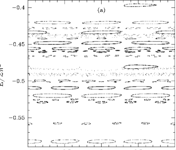
Figure 8: (a) The map of the $67$ comets that survived after $5\times 10^{6}$ Neptune years of the mapping shown in Figure 8. The orbits are stuck to the edges of the resonant islands. (b) Correlation functions $\sigma\,p(\Delta E/\sigma)$ for time intervals $\Delta t=20$, 60, 200 (solid lines). The Gaussian correlation function expected from the diffusion approximation (eq. 17) and the correlation function for a Gaussian random walk with the same boundary conditions as the map are shown by dotted and dashed lines respectively.

3.1 Other planet masses

So far we have explored the Keplerian map for planet mass $m_{p}=5.24\times 10^{-5}$, corresponding to Neptune. Figures 9(a) and (b) show depletion functions for Saturn ($m_{p}=2.86\times 10^{-4}$) and Jupiter ($m_{p}=9.55\times 10^{-4}$). In both cases we calculated time in the corresponding planet years and comets were lost when they either reached semimajor axis $1000$ AU or collided with the Sun ($L\leq 0$). The Saturn and Jupiter maps began with $2\times 10^{6}$ and $10^{7}$ comets respectively. The results for all three planet masses are similar: the number of surviving comets decays approximately exponentially until a time $t_{s}$, and thereafter decays as a power law, $N(t)\propto t^{-k}$ with $k\simeq 1.3$. The time $t_{s}$ appears to be independent of the initial energy: $t_{s}\simeq 4\times 10^{7}$ planet years for Neptune (from Figure 6[b]), $1.7\times 10^{6}$ for Saturn, and $1.5\times 10^{5}$ for Jupiter. These times can be crudely fit by the formula $t_{s}\sim 0.14/m_{p}^{2}$.

Figure 10(a) shows 1000 Jupiter years of the map, for the $47$ comets with initial energy $E/2\pi^{2}=-0.5$ that survived for $2\times 10^{6}$ Jupiter years. Once again, most of the surviving comets are stuck near resonant islands.

To compare the depletion functions for Jupiter, Saturn and Neptune we superimpose these on Figure 10(b) for (approximately) the same initial energy $E/2\pi^{2}\simeq-0.24$. Note that the timescale is planet years.

Figure 9: The depletion functions for the Keplerian map with a planet mass equal to that of Saturn (a) and Jupiter (b). We used different initial energies for the comets, as indicated in the Figures, but in all cases the comets were in the stochastic sea. The comets are assumed to escape when they reach a semimajor axis $1000$ AU or collide with the Sun ($L\leq 0$). The vertical dotted lines represent sticking times defined by equation (21).

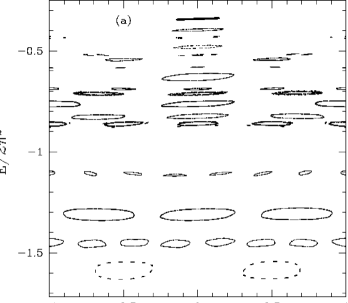
Figure 10: (a) The map of the $47$ comets that survived after $2\times 10^{6}$ planet years of the mapping, with Jupiter’s mass and initial comet energy $E/2\pi^{2}=-0.5$. The orbits are stuck to the edges of the resonant islands. (b) A superposition of the depletion functions for mappings with Jupiter, Saturn and Neptune [from Figures 6(b), 9(a), 9(b)]. The initial comet energy (in the corresponding planet energy units) was approximately the same in each case, $E/2\pi^{2}\simeq-0.24$. The vertical dotted lines represent sticking times defined by equation (21).

4 Discussion

The results of the previous section suggest that the depletion function for the Keplerian mapping, with absorbing boundaries at $0<E_{max}<E<E_{min}$, can be approximately represented in the form

$$N(t) \simeq \exp(-\alpha m_{p}^{2}D_{0}t/P),\qquad t<t_{s}$$ (19)

$$\simeq \beta{\left(t_{s}/t\right)}^{k},\qquad\qquad t>t_{s}.$$ (20)

Here the time $t$ is measured in physical units (e.g. Earth years), $P$ is the planet’s orbital period in Earth years, $\alpha$ and $\beta$ are constants that are approximately independent of planet mass but may depend on the initial energy or angular momentum of the comets, $D_{0}$ is defined by equation (4), and $k\simeq 1.3$. This formula only applies if the escape energy is non-zero. The “sticking time” $t_{s}$ is given by

$$t_{s}=\frac{\log(1/\beta)}{\alpha D_{0}}\frac{P}{m_{p}^{2}}.$$ (21)

We show sticking times calculated by equation (21), with $\alpha\approx 0.04$ and $\beta\approx 10^{-4}$, on Figures 9 and 10(b) as vertical dotted lines.

Our studies of the Keplerian map show that resonance sticking does occur for highly eccentric planet-crossing orbits. The characteristic sticking time, after which resonance sticking dominates the depletion function, is $t_{s}\simeq 2\times 10^{6}$ (Earth) years for Jupiter, $5\times 10^{7}$ years for Saturn, $5\times 10^{9}$ years for Uranus, and $7\times 10^{9}$ years for Neptune (for perihelion distance 0.5 times the planet’s semimajor axis). Thus resonance sticking would be unimportant for a planetary system containing one planet with the mass and semimajor axis of Uranus or Neptune. However, if the planet resembled Jupiter or Saturn, resonance sticking would dominate the long-term behaviour of comets on planet-crossing orbits.

These results invite comparison with long integrations of the orbits of Neptune-crossing objects. Duncan and Levison (1997) followed 2200 test particles on Neptune-crossing orbits for $4\times 10^{9}$ years in the gravitational field of the Sun and the giant planets. They found that on Gyr timescales the depletion function could be described by a law of the form (20) with $k\simeq 1$, normalized so that 1% of their particles survive after 4 Gyr.

These results are reminiscent of the results from the map: there is power-law behaviour at large times, the exponent $k\simeq 1$ is close to the exponent $1.3$ observed in the map, and the surviving comets at the end of the integration were mostly in Neptune resonances, just as in the map. However, our map predicts that sticking is only important for $t>t_{s}=7\times 10^{9}$ years, and that at $t=t_{s}$ only $10^{-4}$ of the initial particles survive, which is smaller by two orders of magnitude. The reason for this discrepancy between the map and direct integrations is unknown; perhaps the enhanced role of resonances reflects the extra degrees of freedom in the integration, which has four planets on eccentric, inclined orbits rather than one on a circular orbit.

To investigate evolution in more realistic planetary systems, we would like to generalize the map to include (i) multiple planets; (ii) eccentric planetary orbits; (iii) dependence of the perturbing Hamiltonian $\kappa$ on energy and angular momentum, not just the azimuthal angle $\psi$ (cf. eq. 10). All of these generalizations are straightforward in principle, although the kick function will depend on more variables and hence requires a more complicated parametrization. When $\kappa$ depends on $E$ and $L$, integrating Hamilton’s equations across the delta-function at $\ell=0$ is generally no longer analytic. One possibility is to use a heuristic form for $\kappa$ chosen so that the integration across $\ell=0$ is analytic. A more general approach is to work with the mixed-variable generating function that describes the canonical transformation induced by the perturbing Hamiltonian across $\ell=0$. Thus if $(L,-E,\varpi,t)$ are the canonical variables just before perihelion passage at $\ell=0$, primes denote the same variables after perihelion passage, and $S(L^{\prime},E^{\prime},\varpi,t)$ is the generating function, then

$$L={\partial S\over\partial\varpi},\quad E=-{\partial S\over\partial t},\quad t^{\prime}=-{\partial S\over\partial E^{\prime}},\quad\varpi^{\prime}={\partial S\over\partial L}.$$ (22)

It is also straightforward to show that

$$S(L^{\prime},E^{\prime},\varpi,t)=L^{\prime}\varpi-E^{\prime}t-m_{p}\kappa(L^{\prime},E^{\prime},\varpi,t)+\hbox{O}(m_{p}^{2}).$$ (23)

Equations (22) are implicit in the post-perihelion variables, but iterative schemes converge rapidly for small planet mass $m_{p}$.

5 Summary

The Keplerian map offers considerable insight into planet-induced evolution of highly eccentric orbits, both because of its simplicity and its computational speed.

The map reveals that the exponential decay in the number of planet-crossing comets predicted by the diffusion or random-walk approximation is replaced at late times by a power-law decay, $N\sim t^{-1.3}$, and that most surviving comets are “stuck” at the edges of resonant islands. Resonance sticking dominates the evolution of comets under Jupiter’s influence after timescales as short as a few Myr.

Sticking to Neptune resonances is not strong enough to explain the remarkably high survival fraction of Neptune-crossing comets (1% after 4 Gyr) found by Duncan and Levison (1997), most likely because the simple map used in this paper does not include eccentric planetary orbits, multiple planets, or dependence of the planetary perturbations on perihelion distance.

An unresolved issue is how small perturbations and dissipative effects (passing stars, non-gravitational forces, etc.) affect the lifetimes of comets that are stuck to resonances.

We thank Martin Duncan, Matt Holman and Norm Murray for discussions. This research was supported in part by NASA grant NAG5-7310.

References

- (1) Arnold, J. R. 1965, The origin of meteorites as small bodies. II. The model, Astrophys. J. 141, 1536–1549
- (2) Bailey, M. E. 1984, The steady-state -distribution and the problem of cometary fading, Mon. Not. Roy. Astron. Soc. 211, 347–368
- (3) Chirikov, B. V., and Vecheslavov, V. V. 1989, Chaotic dynamics of comet Halley, Astron. Astrophys. 221, 146–154
- (4) Duncan, M. J., and Levison, H. F. 1997, A disk of scattered icy objects and the origin of Jupiter-family comets, Science 276, 1670–1672
- (5) Duncan, M., Quinn, T., and Tremaine, S. 1987, The formation and extent of the Solar System comet cloud, Astron. J. 94, 1330–1338
- (6) Everhart, E. 1968, Change in total energy of comets passing through the Solar System, Astron. J. 73, 1039–1052
- (7) Everhart, E. 1977, The evolution of comet orbits perturbed by Uranus and Neptune, in Comets, Asteroids, Meteorites, ed. A. H. Delsemme (Toledo: University of Toledo), 99–104
- (8) Everhart, E. 1979, The shortage of short-period comets in elliptical orbits, in Dynamics of the Solar System, ed. R. L. Duncombe (Dordrecht: Reidel), 273–275
- (9) Froeschlé, C., and Rickman, H. 1980, New Monte Carlo simulations of the orbital evolution of short-period comets and comparison with observations, Astron. Astrophys. 82, 183–194
- (10) Heisler, J., and Tremaine, S. 1986, The influence of the Galactic tidal field on the Oort comet cloud, Icarus 65, 13–26
- (11) Holman, M. J., and Wisdom, J. 1992, Dynamical stability of the outer solar system and the delivery of short period comets, Astron. J. 104, 2022–2029
- (12) Karney, C.F.F. 1983, Long-time correlations in the stochastic regime, Physica 8D 360-80
- (13) Kendall, D. G. 1961, Some problems in the theory of comets, I and II, in Proc. Fourth Berkeley Symposium on Mathematical Statistics and Probability, ed. J. Neyman (Berkeley: University of California Press), 99–147
- (14) Lichtenberg, A. J., and Lieberman, M. A. 1992, Regular and Chaotic Dynamics (New York: Springer)
- (15) Meiss, J. D. 1992, Symplectic maps, variational principles, and transport, Rev. Mod. Phys. 64, 795–848
- (16) Oort, J. H. 1950, The structure of the cloud of comets surrounding the Solar System, and a hypothesis concerning its origin, Bull. Astron. Inst. Netherlands 11, 259–269
- (17) Öpik, E. J. 1976, Interplanetary Encounters (Amsterdam: Elsevier)
- (18) Petrosky, T. 1986, Chaos and cometary clouds in the solar system, Phys. Lett A, 117, 328
- (19) Sagdeev, R. Z., and Zaslavsky, G. M. 1987, Stochasticity in the Kepler problem and a model of possible dynamics of comets in the Oort cloud, Il Nuovo Cimento, 97B, 119–130
- (20) Weissman, P. R. 1978, Physical and dynamical evolution of long-period comets, Ph.D. thesis, University of California, Los Angeles.
- Wiegert and Tremaine (1998) Wiegert, P., and Tremaine, S. 1998, The evolution of long-period comets, submitted to Icarus.
- Whipple (1962) Whipple, F. L. 1962, On the distribution of semimajor axes among comet orbits, Astron. J. 67, 1–9
- Yabushita (1979) Yabushita, S. 1979, A statistical study of the evolution of the orbits of long-period comets, Mon. Not. Roy. Astron. Soc. 187, 445–462
- Yabushita (1980) Yabushita, S. 1980, On exact solutions of diffusion equation in cometary dynamics, Astron. Astrophys. 85, 77–79