[

Statistical Mechanics of Self–Gravitating System : Cluster Expansion Method

Abstract

We study statistical mechanics of the self–gravitating system applying the cluster expansion method developed in solid state physics. By summing infinite series of diagrams, we derive a complex free energy whose imaginary part is related to the relaxation time of the system. Summation of another series yields two–point correlation function whose correlation length is essentially given by the Jeans wavelength of the system.

]

a Introduction

Variety of structures found in the present Universe are thought to be seeded by quantum fluctuations in the very early Universe and evolved through the gravitational interaction in the expanding Universe aided by yet unknown Dark Matter. Though there would be several aspects in the study of the formation of these rich structures, we believe the self–gravity is one of the most intrinsic aspects for the structure formation.

Therefore, in this paper, we would like to study fundamental properties of the self–gravitating system (SGS) from a view point of statistical mechanics. We specify the SGS as a mass distribution which consists of discrete mass points mutually interacting through the force of Newtonian gravity. The contact collisions of the ingredients will be neglected.

The SGS is well known to be unstable and eventually collapses. Then it is widely believed that there is no thermal equilibrium in SGS. However relevant structures would be observed in the intermediate stage of its evolution well before the collapse. Therefore we may have a room to construct statistical mechanics of SGS. Actually there have been many studies dealing with statistical mechanics of SGS[8]. For example, an approach by de Vega et al.[9] considering canonical/grand canonical ensemble of SGS in order to explain the scaling relation in the interstellar medium seems interesting. The instability of SGS requires the inevitable introduction of cutoff in their work. We would like to circumvent this situation allowing complex free energy, whose imaginary part provides dynamical information of the system.

We shall construct statistical mechanics of SGS after the model of classical electron–gas system on uniform ion background. It has the same square–inverse law of force but with opposite signature to SGS. Contrary to the ordinary belief, the correspondence, i.e. the replacement $e^{2}\rightarrow-Gm^{2}$, where $e$ is the charge of electron and $G$ is the Newton’s constant, is quite suggestive if we identify the temperature $T$ as the velocity dispersion of SGS. For example, the Debye wavelength $\lambda_{D}$ corresponds to the Jeans wavelength $\lambda_{J}$, and the plasma frequency is related to the inverse of the free fall time, $\omega_{p}^{2}:=-4\pi Gmn=-1/\tau_{ff}^{2}$. We believe that these correspondences are not merely appearance. Actually, we can calculate the free energy of SGS in the same way as the classical electron gas system by applying the cluster expansion method [10, 11, 12]. Moreover, $n$–point correlation functions are similarly obtained.

b Cluster expansion method

We consider a non–relativistic gas system of $N$ particles with the same mass $m$ in a box of size $L$. The gas is in thermal equilibrium at $T$, where the temperature $T$ is identified with the velocity dispersion $\langle{v^{2}}\rangle$ of the system, i.e. $k_{B}T=m\langle{v^{2}}\rangle/3$, where $k_{B}$ is the Boltzmann’s constant.

We work in the canonical ensemble with the Hamiltonian of the system:

$$H=\sum\limits_{i=1}^{N}{{\vec{p}_{i}^{~{}2}}\over{2m}}+\sum\limits_{1\leq i<j\leq N}{\phi_{ij}},$$ (1)

where $\phi_{ij}$ is a potential through which each particles interact. The partition function for fixed number of particles $N$, volume $V=L^{3}$, and temperature $T$, is given by

$$Z(u) = \mathop{\rm Tr}\nolimits\exp\left[-\beta H+\sum\limits_{i=1}^{N}u(\vec{x}_{i})\right]$$ (2)

$$= {{(2\pi m/\beta)^{3N/2}V^{N}}\over{N!h^{3N}}}e^{W(u)},$$ (3)

$$e^{W(u)} = \int_{V^{N}}{{d^{N}\vec{x}}\over{V^{N}}}\exp\left[{\sum\limits_{i=1}^{N}{u(\vec{x}_{i})}+\sum\limits_{1\leq i<j\leq N}{\varphi_{ij}}}\right],$$ (4)

where $\beta=(k_{B}T)^{-1}$, $h$ is the Planck’s constant, and $\varphi_{ij}:=-\beta\phi_{ij}$. We have introduced a source function $u(\vec{x}_{i})$ for convenience of calculation and integrated over the momenta. By using functional derivative with respect to the source $u(\vec{x}_{i})$, $k$–point correlation functions are given by

$$G(\vec{x}_{1},\cdots,\vec{x}_{k})=\lim_{u\to 0}{{\delta^{k}\ln Z(u)}\over{\delta u(\vec{x}_{1})\cdots\delta u(\vec{x}_{k})}}.$$ (5)

For the calculation of thermodynamic quantities, we introduce the logarithm of the average of the configurational sum setting $u\to 0$:

$$W_{0}:=W(0) = \ln\left\langle\exp\left(\sum\limits_{1\leq i<j\leq N}{\varphi_{ij}}\right)\right\rangle,$$ (6)

where $\left\langle\cdots\right\rangle=V^{-N}\int\!{\cdots d^{N}\vec{x}}$.

The cumulant expansion of $W_{0}$ is possible:

$$W_{0} = \left\langle{\exp\left({\sum\limits_{1\leq i<j\leq N}{\varphi_{ij}}}\right)-1}\right\rangle_{C}$$ (7)

$$= \sum\limits_{\scriptscriptstyle{\nu_{1}\cdots\nu_{M}}\atopwithdelims( ){\mbox{except all }\scriptscriptstyle\nu_{i}=0}\hfill}{{{\left\langle{\varphi_{1}^{\nu_{1}}\varphi_{2}^{\nu_{2}}\cdots\varphi_{M}^{\nu_{M}}}\right\rangle_{C}}\over{\nu_{1}!\cdots\nu_{M}!}}},$$ (9)

where $\left\langle\cdots\right\rangle_{C}$ is a cumulant and $1,2,\cdots,M=N(N-1)/2$ are all the possible pairs of $N$–particles.

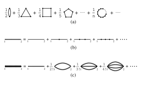
It is convenient to use graphical representations in order to calculate $W_{0}$. An each term in Eq.(9) corresponds to a graph which consists of vertices and lines. Each line terminates at two distinct vertices. A vertex $\vec{x}_{i}$ simply represents an integration position and a line connecting $\vec{x}_{i}$ and $\vec{x}_{j}$ represents an interaction $\varphi_{ij}$. All the elements in a graph are multiplied with each other and integrated over all vertices. This is the cluster expansion method. All the graph which contributes to $\ln Z$ is connected and does not include articulation points which divide the graph into plural pieces, because of the character of the cumulant and the translational invariance of the system.

By expanding with respect to the number density $n=N/V$, $W_{0}$ is reduced to the following form[10, 11, 12].

$$W_{0} = \sum\limits_{k=1}^{\infty}{{{n^{k+1}}\over{(k+1)!}}}\sum\limits_{\mbox{connected}\hfill\atopwithdelims( )\mbox{irreducible}\hfill}\times$$ (12)

$${\int_{V^{k+1}}{\prod\limits_{1\leq i<j\leq k+1}{\left[{{{(\varphi_{ij})^{\nu_{ij}}}\over{\nu_{ij}!}}}\right]d\vec{x}_{1}...d\vec{x}_{k+1}}}},$$

where $\nu_{ij}$ is the number of interaction lines between the vertices $i$ and $j$.

c Application to the self–gravitating system

Let us consider a non–relativistic self–gravitating system where $\phi_{ij}=-Gm^{2}/r_{ij}$ with $r_{ij}=\left|{\vec{x}_{i}-\vec{x}_{j}}\right|$.

Free energy

We shall include the higher orders in $n$ for calculating $W_{0}$. Here we choose a series of graphs which is the lowest order of $\varphi$ in each set of graphs containing $k$ internal vertices. This is equivalent to a sum of all graph which has the topology of a ring (ring approximation shown Fig.1–(a)). This approximation will not be valid for short distances where $\varphi$ grows without bound.

FIG. 1.: A series of cluster expansion: (a) ring graphs. (b) chain graphs. (c) multi–lines of the chain graphs. A symmetric factor is written in the left side of each graph.

A ring graph which contains $k$ vertecies in Eq.(12) corresponds to

$$\int_{V^{k}}{\varphi_{12}\varphi_{23}\cdots\varphi_{k1}d\vec{x}_{1}...d\vec{x}_{k}}=\int_{|\vec{q}|>2\pi/L}{{{d\vec{q}}\over{(2\pi)^{3}}}\left[{\widetilde{\varphi}(\vec{q})}\right]^{k}},$$ (13)

where $\widetilde{\varphi}(\vec{q})={4\pi\beta Gm^{2}}/{\vec{q}^{~{}2}}$ is the Fourier transform of $\varphi(\vec{x})$. $(k-1)!/2$ terms of this kind for each $k$ yield

$$W_{0}= {V\over 2}\int_{|\vec{q}|>2\pi/L}{{{d\vec{q}}\over{(2\pi)^{3}}}}\sum\limits_{k=2}^{\infty}{{{\left[n\widetilde{\varphi}(\vec{q})\right]^{k}}\over k}}$$ (14)

$$= {V\over{4\pi^{2}}}\int_{2\pi/L}^{\infty}{dq\cdot q^{2}}\left[{-{{\kappa^{2}}\over{q^{2}}}-\ln\left({1-{{\kappa^{2}}\over{q^{2}}}}\right)}\right]$$ (15)

$$= {1\over 12\pi^{2}}\Bigl{[}2\pi\kappa^{2}L^{2}+\kappa^{3}L^{3}\ln\Bigl{|}{\kappa L+2\pi\over\kappa L-2\pi}\Bigr{|}$$ (18)

$$\quad\quad+8\pi^{3}\ln\Bigl{|}1-{\kappa^{2}L^{2}\over 4\pi^{2}}\Bigr{|}$$

$$\quad\quad+i\pi\left(\kappa^{3}L^{3}+8\pi^{3}\right)\theta\left(\kappa L-2\pi\right)\Bigr{]},$$

where $\kappa^{2}:=4\pi\beta Gm^{2}n=12\pi^{2}/\lambda_{J}^{2}$ with $\lambda_{J}=\sqrt{\pi\langle v^{2}\rangle/(Gmn)}$ being the Jeans wavelength and $\theta$ is the Heaviside function. For the integration in Eq.(18), we analytically continue $e^{2}$ to $-Gm^{2}$ from the above complex $e^{2}$ plane by the reason under Eq.(20).

We notice that the imaginary part appears for $L>2\pi/\kappa=\lambda_{J}/\sqrt{3}$. This originates from the negative argument in the logarithm for small momentum $q$. The appearance of it apparently indicates the Jeans instability. The thermodynamic limit $N\to\infty,V\to\infty$ with fixed number density $n$, yields the free energy:

$$F = -\beta^{-1}\ln Z(0)$$ (19)

$$= -{N\over\beta}\left[{3\over 2}\ln\left({{2\pi m}\over{\beta h^{2}}}\right)+1-\ln n-{{i\kappa^{3}}\over{12\pi n}}\right].$$ (20)

The above choice of analytical continuation guarantees the positivity of the imaginary part of $F$: The system is truly dissipative rather than anti–dissipative.

In general, the imaginary part of a free energy is directly related with the decay strength of the system $\Gamma$[13]: $\Gamma=(\omega\beta/\pi)$Im$F$, where $-\omega^{2}$ is the negative eigenvalue at the saddle point which divides a metastable region from a stable region. If we identify $\omega$ as the inverse of the free fall time, i.e. $\omega=\tau_{ff}^{-1}=\sqrt{4\pi Gmn}$, the decay strength $\Gamma$ becomes

$$\Gamma={{4\sqrt{3}NG^{2}m^{2}n}\over{\left\langle{v^{2}}\right\rangle^{3/2}}},$$ (21)

which is essentially the inverse of the binary relaxation time[8, 14],

$$\tau_{bc}={{\left\langle{v^{2}}\right\rangle^{3/2}}\over 32\pi G^{2}m^{2}n\ln(N/2)},$$ (22)

except replacing $\ln N$ with $N$.

Contrary to the extensive variables in the conventional thermodynamics, the imaginary part of $F$ apparently is superextensive since ${\rm Im}F\propto n^{3/2}$ but not $\propto n$. Moreover the imaginary part is related to the fluctuation of the system through the fluctuation–dissipation theorem. In this context, it seems interesting to notice that the number $3$ in the above $n^{3/2}$ comes from the spatial dimensionality and $2$ from the inverse–square law of the gravitational force. This reminds us of the Holtsmark distribution of the gravitational force acting in the uniform self–gravitating system [14] or the stable distribution of index $3/2$ [15].

Two–point correlation function

Let us now turn our attention to the correlation functions. One–point correlation function is simply a number: $G_{1}(\vec{x})=N$. The normalized two–point correlation function which is usually used in astrophysics is

$$\xi(r)=G(\vec{x}_{1},\vec{x}_{2})/\left[G(\vec{x}_{1})G(\vec{x}_{2})\right],$$ (23)

where $r=|\vec{x}_{1}-\vec{x}_{2}|$. A similar cluster expansion for $G(\vec{x}_{1},\vec{x}_{2})$ would be

$$G(\vec{x}_{1},\vec{x}_{2}) = N(N-1)\sum\limits_{k=0}^{\infty}{{{n^{k}}\over{k!}}}\sum\limits_{\mbox{connected}}\times$$ (26)

$$\int_{V^{k}}{\prod\limits_{1\leq i<j\leq k+2}{\left[{{{(\varphi_{ij})^{\nu_{ij}}}\over{\nu_{ij}!}}}\right]d\vec{x}_{3}...d\vec{x}_{k+2}}}.$$

We shall include higher orders in $n$ as previous calculation. Therefore, among each set of graphs which contain $k$ internal vertices (excluding both ${\vec{x}_{1}}$ and ${\vec{x}_{2}}$), we choose the lowest order skeleton graph in $\varphi_{ij}$. This is equivalent to a sum of all the graph which has the topology of a chain shown in Fig.1–(b).

$$\overline{\varphi}_{12} = \varphi_{12}+\int_{V}{\varphi_{13}\varphi_{32}d\vec{x}_{3}}$$ (28)

$$\quad\quad\!\!+\int_{V^{2}}{\varphi_{13}\varphi_{34}\varphi_{42}d\vec{x}_{3}d\vec{x}_{4}+\cdots}$$

$$= \int\!{{d\vec{q}}\over{(2\pi)^{3}}}{{\widetilde{\varphi}(\vec{q})}\over{1-n\widetilde{\varphi}(\vec{q})}}\exp\left[i\vec{q}(\vec{x}_{1}-\vec{x}_{2})\right]$$ (29)

$$= {{2\beta Gm^{2}}\over{\pi r}}\int_{0}^{\infty}{d\lambda{{\lambda\sin\lambda}\over{\lambda^{2}-\kappa^{2}r^{2}}}}$$ (30)

$$= \beta Gm^{2}{\cos(\kappa r)\over r}.$$ (31)

Since we have analytically continued from the above complex $e^{2}$ plane in Eq.(18), we should choose the pole at $-\kappa r$ for the integration. Summing over multi–lines of chain graphs shown in Fig.1–(c), we obtain the following function:

$$\widehat{\varphi}_{12} = \overline{\varphi}_{12}+{1\over{2!}}(\overline{\varphi}_{12})^{2}+{1\over{3!}}(\overline{\varphi}_{12})^{3}+{1\over{4!}}(\overline{\varphi}_{12})^{4}+\cdots$$ (32)

$$= \exp(\overline{\varphi}_{12})-1.$$ (33)

Moreover, we should consider mass renormalization for the external vertex. In principle, this is given by sum of all the graph which consists of a cluster around the external vertex $\vec{x}_{1}$. Since infinite summation of this class of graphs at present is technically impossible, we phenomenologically introduce an effective mass. Since the gravitational attractive force balances with the stirring force arising from the velocity dispersion at the length scale $\kappa^{-1}$, the mass inside of this scale is thought to behave collectively. Thus we estimate the effective mass $m^{*}=(4\pi/3)(\kappa^{-1})^{3}nm$, which should be replaced with the mass $m$ at $\vec{x}_{1}$ or at $\vec{x}_{2}$ but not both. Strictly speaking, $m^{*}$ is a parameter in the present phenomenological argument. By replacing $m$ at $\vec{x}_{1}$ in Eq.(31) with $m^{*}$ at $\vec{x}_{1}$, the two–point correlation function becomes $G(\vec{x}_{1},\vec{x}_{2})=N^{2}\left.{\widehat{\varphi}_{12}}\right|_{m_{\mbox{at}\vec{x}_{1}}\to m^{*}_{\mbox{at}\vec{x}_{1}}}$. Finally we obtain the normalized two–point correlation function:

$$\xi(r)=\exp\left[{\cos(\kappa r)\over{3\kappa r}}\right]-1.$$ (34)

The scaling property is manifest: Small scale SGS with large $\kappa$ has the same correlation function as that of large SGS with small $\kappa$.

This function $\xi(r)$ has interesting features. As a function of $s=\kappa r$, it has a unique inflection point at $s=0.440$ when plotted in the Log–Log graph. The slope at $s=0.44$ is $-1.667$ and the magnitude there is $0.986$. Therefore, the inflection point $r_{c}\sim 0.44\kappa^{-1}\sim 0.04\lambda_{J}$ is regarded as the correlation length of SGS.

FIG. 2.: A Log–Log graph of two–pint correlation function: $\xi(s)=\exp\left[\cos(s)/(3s)\right]-1$ (solid line), $\left(s/0.45\right)^{-1.77}$ (broken line), observational data of galaxies [16] (open circle), and observational data of clusters of galaxies [17] (filled circle). These correlation lengths of the observational data are rescaled.

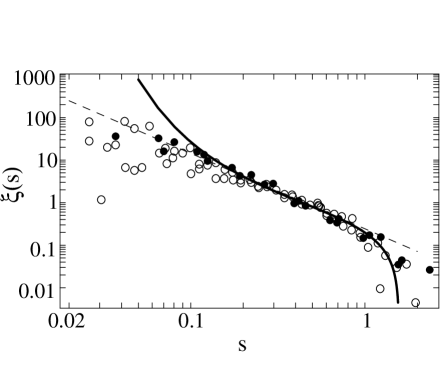
The above two–point correlation function is shown in Fig.2 with typical observational results[16, 17] on top of it. The observation does not exclude our correlation function except small scale region where the interaction $\varphi$ exceeds $1$ and the approximation we used is obviously invalid.

From the observational data[16, 17], the correlation lengths of galaxies and of clusters of galaxies directly read off as $r_{\scriptscriptstyle c}^{\scriptscriptstyle galaxy}\sim 6.2h^{-1}{\rm Mpc}$ and $r_{\scriptscriptstyle c}^{\scriptscriptstyle cluster}\sim 15h^{-1}{\rm Mpc}$ respectively. Since $r_{c}\sim 0.44\kappa^{-1}$ for the two–point correlation function we obtained, we rescaled the observational data: $r\to s=\kappa r$ with $\kappa=1/14~{}h{\rm Mpc}^{-1}$ for galaxies and $\kappa=1/34~{}h{\rm Mpc}^{-1}$ for clusters of galaxies, where $h=H_{0}/\left(100{\rm kms}^{-1}\mbox{Mpc}^{-1}\right)$ with $H_{0}$ being the Hubble constant at the present time. These values of $\kappa$ correspond to $\lambda_{\scriptscriptstyle J}^{\scriptscriptstyle galaxy}\sim 152h^{-1}{\rm Mpc}$ and $\lambda_{\scriptscriptstyle J}^{\scriptscriptstyle cluster}\sim 370h^{-1}{\rm Mpc}$ from the relation given immediately after Eq.(18). On the other hand, typical Jeans lengths calculating from the standard observations for galaxies and for clusters of galaxies are respectively

$$\lambda_{\scriptscriptstyle J}^{\scriptscriptstyle galaxy}=123{\rm Mpc}\Biggl{[} \left({\left\langle{v^{2}}\right\rangle\over 500{\rm kms}^{-1}}\right){\left({2\times 10^{44}{\rm g}\over m}\right)}\times$$ (36)

$${\left({3.7\times 10^{-2}h^{3}{\rm Mpc}^{-3}\over n}\right)}\Biggr{]}^{-1/2},$$

$$\lambda_{\scriptscriptstyle J}^{\scriptscriptstyle cluster}=450{\rm Mpc}\Biggl{[} \left({\left\langle{v^{2}}\right\rangle\over 1000{\rm kms}^{-1}}\right){\left({2\times 10^{47}{\rm g}\over m}\right)}\times$$ (38)

$${\left({1.1\times 10^{-5}h^{3}{\rm Mpc}^{-3}\over n}\right)}\Biggr{]}^{-1/2}.$$

These values of the Jeans lengths are not so far from the above values through two–point correlation function we obtained.

d summary and outlook

Studying the canonical ensemble of the self–gravitating system (SGS), we obtained the complex free energy by summing an infinite series of graph in the cluster expansion method for SGS, Eq.(20). The imaginary part of the free energy yields the decay strength of SGS, Eq.(21). Similar summation of an infinite series of graph yields the universal two–point correlation function Eq.(34) which scales essentially with the Jeans wavelength. The correlation length is linearly proportional to the mean separation of ingredients.

We hope further development will be reported soon, including (a) the higher–point correlation functions, (b) much profound calculation on the complex free energy, (c) systematic argument on the mass renormalization $m^{*}$, (d) the observational tests of our arguments, and (e) the effects of the cosmic expansion and of the Dark matter.