Large-scale Structure from Quantum Fluctuations in the Early Universe

Abstract

A better understanding of the formation of large-scale structure in the Universe is arguably the most pressing question in cosmology. The most compelling and promising theoretical paradigm, Inflation + Cold Dark Matter, holds that the density inhomogeneities that seeded the formation of structure in the Universe originated from quantum fluctuations arising during inflation and that the bulk of the dark matter exists as slowing moving elementary particles (‘cold dark matter’) left over from the earliest, fiery moments. Large redshift surveys (such as the SDSS and 2dF) and high-resolution measurements of CBR anisotropy (to be made by the MAP and Planck Surveyor satellites) have the potential to decisively test Inflation + Cold Dark Matter and to open a window to the very early Universe and fundamental physics.

1 From Quark Soup to Large-scale Structure

The hot big-bang cosmology is so successful that for two decades it has been called the standard cosmology (see e.g., Peebles 1993 or Kolb & Turner 1990). It provides an accounting of the Universe from a fraction of a second after the beginning when the Universe was a hot, smooth soup of quarks and leptons to the present, some $13\,{\rm Gyr}$ later. The observational foundation of the standard cosmology rests upon three strong pillars: the expansion of the Universe; the cosmic microwave background radiation (CBR); and the abundance pattern of the light elements, D, ³He, ⁴He, and ⁷Li, produced seconds after the bang (see e.g., Peebles et al., 1991).

In contrast to the early Universe, the Universe today abounds with structure: galaxies, clusters of galaxies, superclusters, voids and great walls of galaxies stretching across the sky. According to the standard cosmology, all this structure evolved by gravitational amplification of small density inhomogeneities over the past $13\,$Gyr or so. The detection of 30 microKelvin variations in the temperature of the CBR between points on the sky separated by $10^{\circ}$ by the DMR instrument on NASA’s COBE satellite (Smoot et al., 1992) gave the first evidence for the existence of these density perturbations, and further, showed they were of the size needed to account for the observed structure. The COBE results have been followed up many other independent detections on angular scales from $20^{\circ}$ down to a fraction of a degree (Bennett et al., 1997), summarized in Fig. 1.

While the standard cosmology leaves a number of fundamental questions unexplained – the matter/antimatter asymmetry, origin of the smoothness and flatness of the Universe, nature of the big bang itself – the most pressing question involves the initial data for structure formation: the nature and origin of the density inhomogeneities and the quantity and composition of matter and energy in the Universe. Because of powerful and expansive theoretical ideas and an impending avalanche of data, cosmology is poised for a major advance on this front, and with it fundamental physics, because the most promising ideas are inspired by speculations about elementary particle physics at very high energies and short distances.

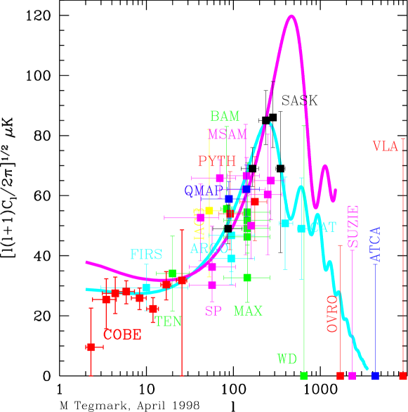
Figure 1: Summary of current CBR anisotropy measurements, where the temperature variation across the sky has been expanded in spherical harmonics, $\mathchar 28942\relax T(\mathchar 28946\relax,\mathchar 28958\relax)=\sum_{i}a_{lm}Y_{lm}$ and $C_{l}\equiv\langle|a_{lm}|^{2}\rangle$. The curves illustrate CDM models with $\Omega_{0}=1$ and $\Omega_{0}=0.3$. Note the preference of the data for a flat Universe (Figure courtesy of M. Tegmark).

a Origin of inhomogeneity

The two most promising ideas for the origin of the seed inhomogeneities are cosmological inflation and cosmological symmetry breaking phase transitions. While both ideas involve the physics of the early Universe, they are orthogonal, conceptually and technically. According to inflation, quantum-mechanical fluctuations in the scalar field driving inflation lead to density perturbations, which then become fluctuations in the local curvature of the Universe during the inflationary epoch. The other early-Universe alternative involves the production of topological defects in a symmetry-breaking phase transition around $10^{-36}\,$sec after the beginning. The defects themselves – monopoles, cosmic strings, or textures – do not directly lead to density perturbations on astrophysically interesting scales. Rather, the conversion of energy into defects causes a pressure perturbation which propagates outward, and much later on, leads to a perturbation in the matter density. (This type of density perturbation is called isocurvature.) I will focus exclusively on the inflationary scenario; the defect scenario is discussed by Turok (1998).

b Nature of the matter and energy in the Universe

The other crucial issue is the quantity and composition of matter and energy in the Universe. The amount of matter that clusters can be measured in a variety of ways: galaxy and cluster mass-to-light ratios, peculiar motions of galaxies, the cluster baryon fraction, and the shape of the power spectrum of density perturbations. At present all methods are consistent with $\Omega_{M}\simeq 0.35\pm 0.07$ (Dekel et al., 1997; Bahcall et al., 1993; Willick et al., 1997); however, the remaining systematic uncertainties are such that it is probably not possible to rule out $\Omega_{M}$ as small as 0.1 or as large as 1. Matter in the form of stars and closely related material contributes a tiny fraction of this, $\Omega_{\rm lum}\simeq 0.003h^{-1}$. The fact that $\Omega_{\rm lum}\ll\Omega_{M}$ implies that most of the matter in the Universe is dark and is only revealed by its gravitational effects. ($\Omega_{i}$ is the fraction of critical density contributed by component $i$, and $h=H_{0}/100\,{\rm km\,s^{-1}}\,{\rm Mpc}^{-1}$. Current measurements of the Hubble constant imply $h=0.65\pm 0.07$).

The abundances of the light elements produced seconds after the bang depends upon the density of ordinary matter (baryons); using the recently determined ratio of deuterium-to-hydrogen in high-redshift hydrogen clouds (Burles & Tytler, 1998a and 1998b), the theory of BBN implies that $\Omega_{B}=(0.02\pm 0.002)h^{-2}\simeq 0.05$. (This lies within the larger concordance interval previously determined from the abundances of all the light elements; see Schramm & Turner, 1998.)

Since $\Omega_{B}\gg\Omega_{\rm lum}$, big-bang nucleosynthesis implies that most of the baryons in the Universe are ‘dark’ – that is, not in the form of bright stars and closely related material (plausible possibilities include diffuse hot and/or warm gas, or dark stars). Further, the fact that $\Omega_{B}$ is significantly smaller than $\Omega_{M}$ strongly indicates that most of the matter is something other than baryons. Elementary-particle physics provides three plausible particle candidates: light neutrinos; an axion of mass around $10^{-5}\,$eV, and a neutralino of mass between 10 GeV and 500 GeV (see e.g., Turner 1993b; Jungman et al., 1996). The axion and the neutralino have a predicted abundance today that is comparable to the critical density; for neutrinos, whose number density today is $113{\,{\rm cm}^{-3}}$, a mass of order $30{\,\rm eV}$ corresponds to the critical density. All three possibilities are predictions made by theories that attempt to go beyond the standard model of particles and unify the forces and particles of Nature.

The total energy density is less well known. Expressed as a fraction of the critical density and denoted by $\Omega_{0}=\sum_{i}\Omega_{i}$ ($i=$ baryons, particle dark matter, vacuum energy, ….), it is related to the spatial curvature,

$$R_{\rm curv}^{2}=H_{0}^{-2}/|\Omega_{0}-1|.$$ (1.1)

The amount of dark matter implies that $\Omega_{0}$ must be greater than 0.2, and the age of the Universe and the anisotropy of the CBR constrain $\Omega_{0}$ to be not much greater than 1. The most powerful measure of the curvature is the position of the first acoustic (or Doppler) peak in the angular power spectrum of CBR anisotropy: $l_{\rm Doppler}\sim 220/\sqrt{\Omega_{0}}$. Current measurements are consistent with $\Omega_{0}=1$; see Fig. 1 and Hancock et al. (1997). Ongoing measurements of anisotropy around $l\sim 200$ (angular scale $\mathchar 28946\relax\sim 100^{\circ}/l\sim 0.5^{\circ}$) may soon settle the question.

If $\Omega_{0}=1$ and $\Omega_{M}=0.3$ there is a third dark-matter puzzle: What is the nature of the component of energy that does not clump with matter and is nearly uniformly distributed? To avoid clumping the ‘X-component’ ($\Omega_{X}=1-\Omega_{M}\sim 0.7$) must be relativistic (Turner & White, 1997); however, relativistic particles per se are out, because they lead to CBR anisotropy that is inconsistent with current data (Lopez et al., 1998) and a Universe that is too youthful (for a radiation-dominated Universe $t_{0}={1\over 2}H_{0}^{-1}$, rather than ${2\over 3}H_{0}^{-1}$ which pertains for a matter-dominated Universe).

The remaining possibility is that the smooth component has negative pressure (is elastic) that is comparable in magnitude to its energy density, $p_{X}\mathrel{\mathchoice{\lower 3.6pt\vbox{\halign{$\mathsurround=0pt\displaystyle\hfil#\hfil$\cr<\crcr\sim\crcr}}}{\lower 3.6pt\vbox{\halign{$\mathsurround=0pt\textstyle\hfil#\hfil$\cr<\crcr\sim\crcr}}}{\lower 3.6pt\vbox{\halign{$\mathsurround=0pt\scriptstyle\hfil#\hfil$\cr<\crcr\sim\crcr}}}{\lower 3.6pt\vbox{\halign{$\mathsurround=0pt\scriptscriptstyle\hfil#\hfil$\cr<\crcr\sim\crcr}}}}-\mathchar 28954\relax_{X}/3$. Plausible examples include: a cosmological constant (or vacuum energy) with $p_{X}=-\mathchar 28954\relax_{X}$ (Turner et al., 1984; Peebles, 1984; Efstathiou et al., 1990), a network of light, frustrated defects (e.g., strings in which case $p_{X}=-\mathchar 28954\relax_{X}/3$; Vilenkin, 1984; Spergel & Pen, 1997), and an evolving scalar field (called quintessence by some) with a time-varying relation between pressure and energy density, $\mathchar 28954\relax={1\over 2}\dot{\mathchar 28958\relax}^{2}+V(\mathchar 28958\relax)$ and $p={1\over 2}\dot{\mathchar 28958\relax}^{2}-V(\mathchar 28958\relax)$ (Freese et al., 1987; Ozer & Taha, 1987; Ratra & Peebles, 1988; Bloomfield-Torres & Waga, 1996; Coble et al., 1996; Caldwell et al., 1998).

A smooth component does not reveal its presence in dynamical measurements and is difficult to detect. It does have a striking signature: an accelerated (rather than decelerated) expansion rate, reflected in Sandage’s deceleration parameter,

$$q_{0}\equiv-{(\ddot{R}/R)\over H_{0}^{2}}={\Omega_{M}\over 2}+{\Omega_{X}\over 2}\,[1+3p_{X}/\mathchar 28954\relax_{X}]<0$$ (1.2)

where $R(t)$ is the cosmic-scale factor. Recent measurements of the magnitude – redshift relation for supernovae of type Ia (SNe1a) indicate accelerated expansion ($q_{0}<0$), with $\Omega_{X}\sim 0.6$ and $p_{X}/\mathchar 28954\relax_{X}\sim-1$ (Riess et al., 1998; Perlmutter et al., 1997).

In ending this brief review of the quantity and composition of matter and energy in the Universe, I cannot resist commenting that, for the very first time, we have a prima facie case for a complete and consistent accounting: The Doppler peak is telling us that $\Omega_{0}=1$; dynamical measurements indicate $\Omega_{M}\sim 1/3$; and SNe1a indicate that $\Omega_{X}\sim 2/3$. And further, the picture that has emerged is consistent with inflation, our most promising scenario for extending the standard cosmology. If this turns out to be correct, 1998 will be remembered as a turning point in our understanding of the Universe.

2 From Quantum Fluctuations to Large-scale Structure

Inflation has revolutionized the way cosmologists view the Universe and provides the current working hypothesis for extending the standard cosmology. It explains how a region of size much, much greater than our Hubble volume could have become smooth and flat without recourse to special initial conditions (Guth 1981), as well as the origin of the density inhomogeneities needed to seed structure (Hawking, 1982; Starobinsky, 1982; Guth & Pi, 1982; and Bardeen et al., 1983). Inflation is based upon well defined, albeit speculative physics – the semi-classical evolution of a weakly coupled scalar field – and this physics may well be connected to the unification of the particles and forces of Nature.

On the negative side, while there are numerous working models of inflation, motivated by a variety of concerns – supersymmetry, superstrings, grand unification and simplicity – there is no standard model of inflation. And a disquieting technical point, in all models of inflation the scalar field that drives inflation must have a very flat potential and must be very weakly coupled to other fields. Most particle physicists find this displeasing or, at the very least, begging for further explanation. The extreme flatness and weak coupling trace directly to the requirement of producing density perturbations of amplitude $10^{-5}$ (for recent reviews of inflation see e.g., Turner, 1997a or Lyth & Riotto, 1998).

It would be nice if there were a standard model of inflation, but there isn’t. What is important, is that almost all inflationary models make three very testable predictions: flat Universe, nearly scale-invariant spectrum of Gaussian density perturbations, and nearly scale-invariant spectrum of gravitational waves. These three predictions allow the inflationary paradigm to be decisively tested. While the gravitational waves are an extremely important test, I do not have space to mention them again here (see e.g., Turner 1997c).

The difference between different models of inflation lies in the scalar-field potential; once the scalar-field potential is specified, the story is the same. Inflation begins with the scalar field displaced from the minimum of its potential (for whatever reason); as it evolves toward the potential-energy minimum the scalar-field potential energy drives a nearly exponential expansion. In most models, the time required to evolve to the minimum is many hundreds or thousands of Hubble times, during which the scale factor of the Universe grows by an enormous factor. When the scalar field nears the minimum of its potential, its evolution accelerates and it rapidly oscillates about the minimum. ‘The graceful exit’ from the inflationary era occurs as the original potential energy, which now resides in coherent scalar-field oscillations, decays into relativistic particles, which through interactions eventually thermalize, creating the heat of the hot big-bang model.

The tremendous expansion that occurs during inflation is key to its beneficial effects and robust predictions: A small, subhorizon-sized bit of the Universe can grow large enough to encompass the entire observable Universe and much more. The same small bit of the Universe is smaller than its radius of curvature and appears flat; this relationship is unaffected by the expansion since then and so the Hubble radius today is much, much smaller than the curvature radius, implying $\Omega_{0}=1$ (recall, $R_{\rm curv}=H_{0}^{-1}/|\Omega_{0}-1|^{1/2}$). Lastly, the tremendous expansion stretches quantum fluctuations on truly microscopic scales ($\mathrel{\mathchoice{\lower 3.6pt\vbox{\halign{$\mathsurround=0pt\displaystyle\hfil#\hfil$\cr<\crcr\sim\crcr}}}{\lower 3.6pt\vbox{\halign{$\mathsurround=0pt\textstyle\hfil#\hfil$\cr<\crcr\sim\crcr}}}{\lower 3.6pt\vbox{\halign{$\mathsurround=0pt\scriptstyle\hfil#\hfil$\cr<\crcr\sim\crcr}}}{\lower 3.6pt\vbox{\halign{$\mathsurround=0pt\scriptscriptstyle\hfil#\hfil$\cr<\crcr\sim\crcr}}}}10^{-23}\,{\rm cm}$) to astrophysical scales ($\mathrel{\mathchoice{\lower 3.6pt\vbox{\halign{$\mathsurround=0pt\displaystyle\hfil#\hfil$\cr>\crcr\sim\crcr}}}{\lower 3.6pt\vbox{\halign{$\mathsurround=0pt\textstyle\hfil#\hfil$\cr>\crcr\sim\crcr}}}{\lower 3.6pt\vbox{\halign{$\mathsurround=0pt\scriptstyle\hfil#\hfil$\cr>\crcr\sim\crcr}}}{\lower 3.6pt\vbox{\halign{$\mathsurround=0pt\scriptscriptstyle\hfil#\hfil$\cr>\crcr\sim\crcr}}}}\,{\rm Mpc}$).

The accelerated expansion associated with inflation is crucial. If, and only if, the expansion accelerates (i.e., $\ddot{R}>0$), can a comoving scale begin smaller than the horizon and grow larger. In the standard cosmology, the expansion is always decelerating, and all comoving scales (e.g., the scale corresponding to the presently observable Universe) begin larger than the horizon scale (set by the inverse of the expansion rate $H^{-1}$) and then cross inside the horizon. Thus, objects from galaxies to the presently observable Universe were much larger than the horizon during the earliest moments and outside the sphere of causal influence. Inflation changes that: these objects begin smaller than the horizon where microphysics can affect them and then cross outside the horizon during inflation.

Accelerated expansion makes it kinematically possible to create density inhomogeneities on astrophysical interesting scales, and the quantum fluctuations associated with the deSitter space of accelerated expansion provide the dynamical mechanism. Quantum fluctuations in the scalar field that drives inflation, whose amplitude is set by the Gibbons–Hawking temperature $H/2\mathchar 28953\relax$, lead to energy density fluctuations $\mathchar 28942\relax\mathchar 28954\relax=V^{\prime}\Delta\mathchar 28958\relax=V^{\prime}H/2\mathchar 28953\relax$. As each scale, from galaxies to clusters to the present Hubble scale, crosses outside the horizon, these perturbations become fluctuations in the curvature of the Universe.

The curvature perturbations created by inflation are characterized by two important features: 1) they are almost scale-invariant, which refers to the fluctuations in the gravitational potential being independent of scale – and not the density perturbations themselves; 2) because they arise from fluctuations in an essentially noninteracting quantum field, their statistical properties are that of a Gaussian random field.

Scale invariance specifies the dependence of the spectrum of density perturbations upon scale. The normalization (overall amplitude) depends upon the specific inflationary model (i.e., scalar-field potential). Ignoring numerical factors for the moment, the fluctuation amplitude is given by: $\mathchar 28942\relax\mathchar 28958\relax\simeq(\mathchar 28942\relax\mathchar 28954\relax/\mathchar 28954\relax)_{\rm HOR}\sim V^{3/2}/m_{\rm PL}^{3}V^{\prime}$. (The amplitude of the density perturbation on a given scale at horizon crossing is equal to the fluctuation in the gravitational potential $\mathchar 28942\relax\mathchar 28958\relax$.) To be consistent with the COBE measurement of CBR anisotropy on the $10^{\circ}$ scale, $\mathchar 28942\relax\mathchar 28958\relax$ must be around $2\times 10^{-5}$. Not only did COBE produce the first evidence for the existence of the density perturbations that seeded all structure, but also, for a theory like inflation that predicts the shape of the spectrum of density perturbations, it provides the overall normalization that fixes the amplitude of density perturbations on all scales (see Fig. 2). The COBE normalization began precision testing of inflation.

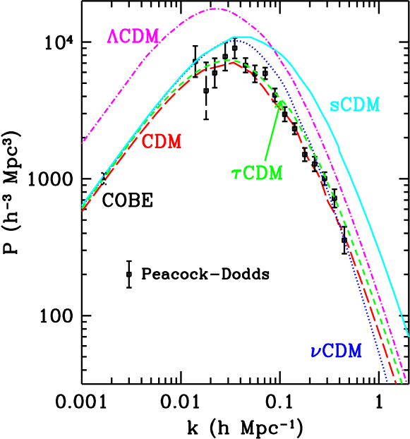
Figure 2: Summary of measurements of the present power spectrum derived from redshift surveys (Peacock & Dodds, 1994) and the predictions of different COBE-normalized CDM models. Because of the possibility that light does not faithfully trace mass (i.e., biasing), the shape of the spectrum is most important in constraining models.

3 Testing Inflation + CDM in the Era of Precision Cosmology

The inflationary predictions of a flat Universe and scale-invariant density perturbations, together with the failure of the hot dark matter theory of structure formation, make cold dark matter (CDM) a key prediction and a powerful means of testing inflation. The key elements of CDM are: 1) Gaussian scale-invariant density perturbations; and 2) dark matter whose primary constituent is slowly-moving, very weakly interacting particles such as axions or neutralinos. CDM is hierarchical in the sense that structure forms from the ‘bottom up’ – galaxies (at redshifts of a few), followed by clusters of galaxies (redshifts of one or less) and finally superclusters (today) (see e.g., Blumenthal et al., 1984).

CDM is generally consistent with the key tests that have been carried out thus far: anisotropy of the CBR on angular scales from less than a degree to $100^{\circ}$, measurements of the distribution of galaxies today, and studies of the evolution of galaxies and clusters (see e.g., Steidel, 1998). This is no mean feat; at present, CDM is the only theory for structure formation that is still viable: the theories based upon defects as the seeds for structure are strongly disfavored by a combination of CBR anisotropy and the power spectrum of inhomogeneity today (Pen et al., 1997; Allen et al. 1997) and Peebles’ “baryon only” model (Peebles, 1987) with isocurvature perturbations (PIB) was ruled out by CBR anisotropy several years ago.

As we look forward to the abundance (avalanche!) of high-quality observations that will test Inflation + CDM, we have to make sure the predictions of the theory match the precision of the data. In so doing, CDM + Inflation becomes a ten (or more) parameter theory. For astrophysicists, and especially cosmologists, this is daunting, as it may seem that a ten-parameter theory can be made to fit any set of observations. This is not the case when one has the quality and quantity of data that will be coming. The standard model of particle physics offers an excellent example: it is a nineteen-parameter theory and because of the high-quality of data from experiments at Fermilab’s Tevatron, SLAC’s SLC, CERN’s LEP and other facilities it has been rigorously tested and the parameters measured to a precision of better than 1% in some cases. My worry as an inflationist is not that many different sets of parameters will fit the upcoming data, but rather that no set of parameters will!

In fact, the ten parameters of CDM + Inflation are an opportunity rather than a curse: Because the parameters depend upon the underlying inflationary model and fundamental aspects of the Universe, we have the very real possibility of learning much about the Universe and inflation. The ten parameters can be organized into two groups: cosmological and dark-matter (Dodelson et al., 1996).

Cosmological Parameters

1. $h$, the Hubble constant in units of $100\,{\rm km\,s^{-1}}\,{\rm Mpc}^{-1}$.

2. $\Omega_{B}h^{2}$, the baryon density. Primeval deuterium measurements and together with the theory of BBN imply: $\Omega_{B}h^{2}=0.02\pm 0.002$.

3. $n$, the power-law index of the scalar density perturbations. CBR measurements indicate $n=1.1\pm 0.2$; $n=1$ corresponds to scale-invariant density perturbations. Several popular inflationary models predict $n\simeq 0.95$; range of predictions runs from $0.7$ to $1.2$ (Lyth & Riotto, 1996; Huterer & Turner, 1998).

4. $dn/d\ln k$, “running” of the scalar index with comoving scale ($k=$ wavenumber). Inflationary models predict a value of ${\cal O}(\pm 10^{-3})$ or smaller (Kosowsky & Turner, 1995).

5. $S$, the overall amplitude squared of density perturbations, quantified by their contribution to the variance of the CBR quadrupole anisotropy.

6. $T$, the overall amplitude squared of gravity waves, quantified by their contribution to the variance of the CBR quadrupole anisotropy. Note, the COBE normalization determines $T+S$ (see below).

7. $n_{T}$, the power-law index of the gravity wave spectrum. Scale-invariance corresponds to $n_{T}=0$; for inflation, $n_{T}$ is given by $-{1\over 7}{T\over S}$.

Dark-matter Parameters

1. $\Omega_{\mathchar 28951\relax}$, the fraction of critical density in neutrinos ($=\sum_{i}m_{\mathchar 28951\relax_{i}}/90h^{2}$). While the hot dark matter theory of structure formation is not viable, it is possible that a small fraction of the matter density exists in the form of neutrinos. Further, small – but nonzero – neutrino masses are a generic prediction of theories that unify the strong, weak and electromagnetic interactions.

2. $\Omega_{X}$, the fraction of critical density in a smooth component of unknown composition and negative pressure ($w_{X}\mathrel{\mathchoice{\lower 3.6pt\vbox{\halign{$\mathsurround=0pt\displaystyle\hfil#\hfil$\cr<\crcr\sim\crcr}}}{\lower 3.6pt\vbox{\halign{$\mathsurround=0pt\textstyle\hfil#\hfil$\cr<\crcr\sim\crcr}}}{\lower 3.6pt\vbox{\halign{$\mathsurround=0pt\scriptstyle\hfil#\hfil$\cr<\crcr\sim\crcr}}}{\lower 3.6pt\vbox{\halign{$\mathsurround=0pt\scriptscriptstyle\hfil#\hfil$\cr<\crcr\sim\crcr}}}}-0.3$). There is mounting evidence for such a component, with the simplest example being a cosmological constant ($w_{X}=-1$).

3. $g_{*}$, the quantity that counts the number of ultra-relativistic degrees of freedom (around the time of matter-radiation equality). The standard cosmology/standard model of particle physics predicts $g_{*}=3.3626$ (photons in the CBR + 3 massless neutrino species with temperature $(4/11)^{1/3}$ times that of the photons). The amount of radiation controls when the Universe became matter dominated and thus affects the present spectrum of density inhomogeneity.

Since $\Omega_{0}=1.0$ is taken to be an inflationary prediction, $\Omega_{\rm CDM}=1-\Omega_{\mathchar 28951\relax}-\Omega_{B}-\Omega_{X}$. Additional parameters can be added (e.g., $\Omega_{0}$, $w_{X}$, the epoch of reionization). Bond’s list totals nineteen, coincidentally equal to the number of parameters in the standard model of particle physics (Bond & Jaffe, 1998). The main point is that testing inflation + CDM requires precision predictions, which in turn, depend on ten or so parameters.

As mentioned, the parameters involving density and gravity-wave perturbations depend directly upon the inflationary potential. In particular, they can be expressed in terms of the potential and its first three derivatives (see e.g., Turner, 1997a):

$$S \equiv {5\langle|a_{2m}|^{2}\rangle\over 4\mathchar 28953\relax}\simeq 2.2\,{V_{*}/m_{\rm Pl}^{4}\over(m_{\rm Pl}V_{*}^{\prime}/V_{*})^{2}}$$ (3.3)

$$n-1 = -{1\over 8\mathchar 28953\relax}\left({{m_{\rm Pl}}V^{\prime}_{*}\over V_{*}}\right)^{2}+{{m_{\rm Pl}}\over 4\mathchar 28953\relax}\left({{m_{\rm Pl}}V_{*}^{\prime}\over V_{*}}\right)^{\prime}$$ (3.4)

$${dn\over d\ln k} = -{1\over 32\mathchar 28953\relax^{2}}\left({{m_{\rm Pl}}^{3}V_{*}^{\prime\prime\prime}\over V_{*}}\right)\left({{m_{\rm Pl}}V_{*}^{\prime}\over V_{*}}\right)$$ (3.5)

$$\hskip 28.45274pt+{1\over 8\mathchar 28953\relax^{2}}\left({{m_{\rm Pl}}^{2}V_{*}^{\prime\prime}\over V_{*}}\right)\left({{m_{\rm Pl}}V_{*}^{\prime}\over V_{*}}\right)^{2}-{3\over 32\mathchar 28953\relax^{2}}\left({m_{\rm Pl}}{V_{*}^{\prime}\over V_{*}}\right)^{4}$$

$$T \equiv {5\langle|a_{2m}|^{2}\rangle\over 4\mathchar 28953\relax}=0.61(V_{*}/m_{\rm Pl}^{4})$$ (3.6)

$$n_{T} = -{1\over 8\mathchar 28953\relax}\left({{m_{\rm Pl}}V^{\prime}_{*}\over V_{*}}\right)^{2}$$ (3.7)

where $V(\mathchar 28958\relax)$ is the inflationary potential, prime denotes $d/d\mathchar 28958\relax$, and $V_{*}$ is the value of the scalar potential when the present horizon scale crossed outside the horizon during inflation. These expressions are given to lowest-order in the deviation from scale invariance (i.e., $n-1$ and $n_{T}$), and assume a matter-dominated Universe today; the next-order corrections have been calculated (Liddle & Turner, 1994) and the analogous expressions, including the possibility of a cosmological constant, have been computed (Turner & White, 1996).

Bunn & White (1997) have used the COBE four-year dataset to determine $S$ as a function of $T/S$ and $n-1$; they find

$${V_{*}/m_{\rm Pl}^{4}\over(m_{\rm Pl}V_{*}^{\prime}/V_{*})^{2}}\left(={S\over 2.2}\right)=(1.7\pm 0.2)\times 10^{-11}\,{\exp[-2.02(n-1)]\over\sqrt{1+{2\over 3}{T\over S}}}$$ (3.8)

From which it follows that

$$V_{*}<6\times 10^{-11}{m_{\rm Pl}}^{4},$$ (3.9)

equivalently, $V_{*}^{1/4}<3.4\times 10^{16}\,{\rm GeV}$. This indicates that inflation must involve energies much smaller than the Planck scale. (To be more precise, inflation could have begun at a much higher energy scale, but the portion of inflation relevant for us, i.e., the last 60 or so e-folds, occurred at an energy scale much smaller than the Planck energy.)

This normalization can also be expressed in terms of the horizon-crossing amplitude for the comoving scale $k=H_{0}$:

$$\mathchar 28942\relax_{H}(k=H_{0})\equiv\left[{k^{3/2}|\mathchar 28942\relax_{k}|\over\sqrt{2\mathchar 28953\relax^{2}}}\right]_{k=H_{0}}=1.9\times 10^{-5}\,{\exp[-1.01(n-1)]\over\sqrt{1+{2\over 3}\,{T\over S}}}.$$ (3.10)

That is, for $n=1$ and $T/S=0$, the COBE normalization implies that the horizon-crossing amplitude of density perturbations is about $2\times 10^{-5}$.

Finally, it should be noted that the ‘tensor tilt,’ deviation of $n_{T}$ from 0, and the ‘scalar tilt,’ deviation of $n-1$ from zero, are not in general equal; they differ by the rate of change of the steepness. The tensor tilt and the ratio $T/S$ are related: $n_{T}=-{1\over 7}{T\over S}$, which provides a potential consistency test of inflation.

a Present status of Inflation + CDM

A useful way to organize the different CDM models is by their dark-matter content; within each CDM family, the cosmological parameters vary. One list of models is:

1. sCDM (for simple): Only CDM and baryons; no additional radiation ($g_{*}=3.36$). The original standard CDM is a member of this family ($h=0.50$, $n=1.00$, $\Omega_{B}=0.05$), but is now ruled out (see Fig. 3).

2. $\mathchar 28956\relax$CDM: This model has extra radiation, e.g., produced by the decay of an unstable massive tau neutrino (hence the name); here we take $g_{*}=7.45$.

3. $\mathchar 28951\relax$CDM (for neutrinos): This model has a dash of hot dark matter; here we take $\Omega_{\mathchar 28951\relax}=0.2$ (about 5 eV worth of neutrinos).

4. $\Lambda$CDM (for cosmological constant): This model has a smooth component in the form of a cosmological constant; here we take $\Omega_{\Lambda}=0.6$.

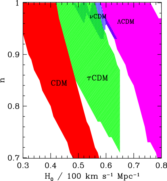
Figure 3: Summary of viable CDM models, based upon CBR anisotropy and determinations of the present power spectrum of inhomogeneity (Dodelson et al., 1996).

Figure 3 summarizes the viability of these different CDM models, based upon CBR measurements and current determinations of the present power spectrum of inhomogeneity (derived from redshift surveys). sCDM is only viable for low values of the Hubble constant (less than $55\,{\rm km\,s^{-1}}\,{\rm Mpc}^{-1}$) and/or significant tilt (deviation from scale invariance); the region of viability for $\mathchar 28956\relax$CDM is similar to sCDM, but shifted to larger values of the Hubble constant (as large as $65\,{\rm km\,s^{-1}}\,{\rm Mpc}^{-1}$). $\mathchar 28951\relax$CDM has an island of viability around $H_{0}\sim 60\,{\rm km\,s^{-1}}\,{\rm Mpc}^{-1}$ and $n\sim 0.95$. $\Lambda$CDM can tolerate the largest values of the Hubble constant.

Considering other relevant data too – e.g., age of the Universe, determinations of $\Omega_{M}$, measurements of the Hubble constant, and limits to $\Omega_{\Lambda}$ – $\Lambda$CDM emerges as the hands-down-winner of ‘best-fit CDM model’ (Krauss & Turner, 1995; Ostriker & Steinhardt, 1995; Liddle et al., 1996; Turner, 1997b). Moreover, not only is it consistent with all the data (see Fig. 4), but also its ‘smoking gun signature,’ negative $q_{0}$, has apparently been confirmed (Riess et al., 1998; Perlmutter et al., 1997). Given the possible systematic uncertainties in the SNe1a data and other measurements, it is premature to conclude that $\Lambda$CDM is anything but the model to take aim at.

Figure 4: Constraints used to determine the best-fit CDM model: PS = large-scale structure + CBR anisotropy; AGE = age of the Universe; CBF = cluster-baryon fraction; and $H_{0}$= Hubble constant measurements. The best-fit model, indicated by the darkest region, has $h\simeq 0.60-0.65$ and $\Omega_{\Lambda}\simeq 0.55-0.65$ (Krauss & Turner 1995; Turner, 1997c).

4 Testing Inflation with Maps of the Universe

Over the next decade two maps of the Universe with unprecedented precision will be made. The first, derived from high-resolution (around $0.1^{\circ}$) measurements of the CBR by NASA’s MAP and ESA’s Planck satellites, will provide a snapshot of the Universe at a simpler time, 300,000 yrs after the beginning when the average level of inhomogeneity was much less than 1%. The second, derived from the more than one million galaxy redshifts to be gathered by the SDSS and 2dF teams, will provide an accurate picture of the structure that exists in the Universe today. The two maps are complementary and together have great leverage to settle the question of how structure in the Universe originated as well as to probe cosmology and fundamental physics.

The SDSS and 2dF redshift surveys will probe the Universe on scales from less than $1h^{-1}\,{\rm Mpc}$ to $500h^{-1}\,{\rm Mpc}$. The structure that exists today depends not only upon the primordial spectrum of inhomogeneity, but also upon the composition of the dark matter, cosmological parameters and the complicated astrophysical relationship between the present distribution of light and mass. CBR anisotropy probes the primeval spectrum of inhomogeneity on scales from $10h^{-1}\,{\rm Mpc}$ to $10^{4}h^{-1}\,{\rm Mpc}$. Together, they will probe inhomogeneity over almost six orders-of-magnitude in length.

The power of these two maps when used together has been stressed by a number of authors (see e.g., Eisenstein et al., 1998). I mention but a few examples. CBR anisotropy should determine $\Omega_{0}$ and $h$ to a precision of better than 1%; large-scale structure can accurately determine $\Omega_{M}h$ (the shape parameter). Together, they determine accurately $\Omega_{M}$, $\Omega_{X}$ and $h$. The effect of a neutrino mass as small as a few tenths of an eV should be detectable by a combination of redshift data and CBR anisotropy (Hu et al., 1998). The two maps will both probe inhomogeneity on scales of $10h^{-1}\,{\rm Mpc}$ to around $500h^{-1}\,{\rm Mpc}$, which will allow the mismatch between the distribution of light and mass (biasing) to be addressed.

a Looking ‘out’ to see ‘in’

Inflation and cold dark matter are a bold attempt to extend our knowledge of the Universe to within $10^{-32}\,{\rm sec}$ of the bang. The scenario is deeply rooted in fundamental physics. I am confident that redshift surveys, CBR anisotropy and a host of other cosmological observations and laboratory experiments will decisively test inflation + CDM. Further, I believe prospects for discriminating among the different CDM models and models of inflation are excellent. If inflation + CDM is shown to be correct, an important aspect of the standard cosmology – the origin and evolution of structure – will have been resolved and a window to the early moments of the Universe and physics at very high energies will have been opened.

While the window has not been opened yet, I would like to end with one example of what one could hope to learn. As discussed earlier, $S$, $n-1$, $T/S$ and $n_{T}$ are related to the inflationary potential and its first two derivatives. If one can measure the power-law index of the density perturbations and the amplitudes of the density and gravity-wave perturbations, one can recover the value of the potential and its first two derivatives (see e.g., Turner 1993a; Lidsey et al. 1997)

$$V_{*} = 1.65T\,{m_{\rm Pl}}^{4},$$ (4.11)

$$V_{*}^{\prime} = \pm\sqrt{{8\mathchar 28953\relax\over 7}\,{T\over S}}\,V_{*}/{m_{\rm Pl}},$$ (4.12)

$$V_{*}^{\prime\prime} = 4\mathchar 28953\relax\left[(n-1)+{3\over 7}{T\over S}\right]\,V_{*}/{m_{\rm Pl}}^{2},$$ (4.13)

where the sign of $V^{\prime}$ is indeterminate (under the redefinition $\mathchar 28958\relax\leftrightarrow-\mathchar 28958\relax$ the sign changes). If, in addition, the gravity-wave spectral index can also be measured the consistency relation, $T/S=-7n_{T}$, can be used to test inflation. Reconstruction of the inflationary scalar potential would shed light both on inflation as well as physics at energies of the order of $10^{14}\,{\rm GeV}$. Already, the success of Inflation + CDM is evidence for physics beyond the standard model of particle physics.

References

- 1
- 2 Allen, B., Caldwell, R. R., Dodelson, S., Knox, L., Shellard, E. P. S., & Stebbins, A. 1997 Cosmic Microwave Background anisotropy induced by cosmic strings on angular scales greater than about . Phys. Rev. Lett. 79, 2624-2627.
- 3
- 4 Bahcall, N.A. et al. 1993 Astrophys. J. 415, L17.
- 5
- 6 Bardeen, J., Steinhardt, P.J., & Turner, M.S. 1983 Spontaneous creation of almost scale-free density perturbations in an inflationary universe. Phys. Rev. D 28, 679-693.
- 7
- 8 Bennett, C. et al. 1997 Physics Today Nov., 32.
- 9
- 10 Bloomfield-Torres, L.F. & Waga, I. 1996 Mon. Not. R. Astron. Soc. 279, 712.
- 11
- 12 Blumenthal, G. R., Faber, S. M., Primack, J. R., & Rees, M. J. 1984 Formation of galaxies and large-scale structure with cold dark matter. Nature 311, 517.
- 13
- 14 Bond, J.R. & Jaffe, A. 1998 in this volume.
- 15
- 16 Bucher, M., Goldhaber, A. S., & Turok, N. 1995 Open universe from inflation. Phys. Rev. D 52, 3314.
- 17
- 18 Bunn, E. F. & White, M. 1997 The 4-year COBE normalization and large-scale structure. Astrophys. J. 480, 6-21.
- 19
- 20 Burles, S. & Tytler, D. 1998a The deuterium abundance toward Q1937-1009. Astrophys. J. 499, 699-712.
- 21
- 22 Burles, S. & Tytler, D. 1998b Astrophys. J. in press.
- 23
- 24 Caldwell, R., Dave, R., & Steinhardt, P.J. 1998 Cosmological imprint of an energy component with general equation of state. Phys. Rev. Lett. 80, 1582-1585.
- 25
- 26 Coble, K., Dodelson, S., & Frieman, J. A. 1996 Dynamical models of structure formation. Phys. Rev. D 55, 1851.
- 27
- 28 Dekel, A. et al. 1997. In Critical dialogues in cosmology (ed. N. Turok), p.175. Singapore:World Scientific.
- 29
- 30 Dodelson, S. et al. 1996 Science 274, 69.
- 31
- 32 Efstathiou, G., Sutherland, W.J., & Maddox, S. J. 1990 The cosmological constant and cold dark matter. Nature 348, 705-707.
- 33
- 34 Eisenstein, D. J., Hu, W., & Tegmark, M. 1998 Cosmic complementarity: H0 and from combining CMB experiments and redshift surveys. Astrophys. J., submitted (astro-ph/9805239).
- 35
- 36 Freese, K. et al. 1987 Nucl. Phys. B 287, 797.
- 37
- 38 Guth, A.H. 1981 Inflationary universe: A possible solution to the horizon and flatness problems. Phys. Rev. D 23, 347.
- 39
- 40 Guth, A.H. & Pi, S.-Y. 1982 Fluctuations in the new inflationary universe. Phys. Rev. Lett. 49, 1110-1113.
- 41
- 42 Hancock et al. 1998 Mon. Not. R. Astron. Soc., in press (astro-ph/9708254).
- 43
- 44 Hawking, S.W. 1982 The development of inequalities in a single bubble inflationary universe. Phys. Lett. B 115, 295-297.
- 45
- 46 Hu, W., Eisenstein, D. J., & Tegmark, M. 1998 Weighing neutrinos with galaxy surveys. Phys. Rev. Lett. 80, 5255-5258.
- 47
- 48 Huterer, D. & Turner, M.S. 1998, in preparation.
- 49
- 50 Jungman, G. et al. 1996 Phys. Rep. 267, 195.
- 51
- 52 Kajita, T. (for the Super-Kamiokande Collaboration) 1998, presented at Neutrino 98 (Takayama, Japan, June 4-9).
- 53
- 54 Kolb, E.W. & Turner, M.S. 1990 The early universe. Redwood City, CA:Addison-Wesley.
- 55
- 56 Kosowsky, A. & Turner, M.S. 1995 CBR anisotropy and the running of the scalar spectral index. Phys. Rev. D 52, R1739.
- 57
- 58 Krauss, L. & Turner, M.S. 1995 The cosmological constant is back. Gen. Rel. Grav. 27, 1137.
- 59
- 60 Liddle, A.R. et al. 1996 Mon. Not. R. astron. Soc. 282, 281.
- 61
- 62 Liddle, A.R. & Turner, M.S. 1994 Second-order reconstruction of the inflationary potential. Physical Review D 50, 758.
- 63
- 64 Lidsey, J. et al. 1997 Rev. Mod. Phys. 69, 373.
- 65
- 66 Linde, A.D. & Mezhlumian, A. 1995 Inflation with 1. Phys. Rev. D 52, 6789-6804.
- 67
- 68 Lopez, R. E., Dodelson, S., Scherrer, R. J., & Turner, M. S. 1998 Probing unstable massive neutrinos with current CMB observations. astro-ph/9806116.
- 69
- 70 Lyth, D. H. & Riotto, A. 1998 Particle physics models of inflation and the cosmological density perturbation. Phys. Rep., in press (hep-th/9609431 and 9807278).
- 71
- 72 Ostriker, J.P. & Steinhardt, P.J. 1995 Nature 377, 600.
- 73
- 74 Ozer, M. & Taha, M.O. 1987 Nucl. Phys. B 287, 776.
- 75
- 76 Peacock, J. & Dodds, S. 1994 Reconstructing the linear power spectrum of cosmological mass fluctuations. Mon. Not. R. Astron. Soc. 267, 1020-1034.
- 77
- 78 Peebles, P.J.E. 1984 Astrophys. J. 284, 439.
- 79
- 80 Peebles, P.J.E. 1987 Origin of the large-scale galaxy peculiar velocity field: A miniature isocurvature model. Nature 327, 210-211.
- 81
- 82 Peebles, P.J.E. 1993 Principles of physical cosmology. Princeton NJ:Princeton Univ. Press.
- 83
- 84 Peebles, P.J.E., Schramm, D. N., Turner, E. L., & Kron, R.G. 1991 The case for the relativistic hot big bang cosmology. Nature 352, 769-776.
- 85
- 86 Pen, U.-L. et al. 1997 Phys. Rev. Lett. 79, 1611.
- 87
- 88 Perlmutter, S. et al. 1997 B.A.A.S. 5, 1351.
- 89
- 90 Ratra, B. & Peebles, P.J.E. 1988 Cosmological consequences of a rolling homogeneous scalar field. Phys. Rev. D 37, 3406-3427.
- 91
- 92 Riess, A. et al. 1998 Astron. J., in press.
- 93
- 94 Schramm, D.N. & Turner, M.S. 1998 Big bang nucleosynthesis enters the precision era. Rev. Mod. Phys. 70, 303.
- 95
- 96 Smoot, G., et al. 1992 Structure in the COBE differential microwave radiometer first year maps. Astrophys. J. 396, L1-L6.
- 97
- 98 Spergel, D. N. & Pen, U.-L. 1997 String-dominated universe cosmology. Astrophys. J. 491, L67.
- 99
- 100 Starobinsky, A. A. 1982 Dynamics of phase transition in the new inflationary universe scenario and generation of perturbations. Phys. Lett. B 117, 175.
- 101
- 102 Steidel, C. 1998 in this volume.
- 103
- 104 Turner, M.S. 1993 Recovering the inflationary potential. Phys. Rev. D 48, 5539.
- 105
- 106 Turner, M.S. 1993 Dark matter: Theoretical perspectives. Proc. Natl. Acad. Sci. 90, 4827.
- 107
- 108 Turner, M.S. 1997a. In Generation of cosmological large-scale structure (eds. D.N. Schramm and P. Galeotti), p.153. Dordrecht:Kluwer.
- 109
- 110 Turner, M.S. 1997b The case for CDM. In Critical dialogues in cosmology (ed. N. Turok), p. 555. Singapore:World Scientific.
- 111
- 112 Turner, M.S. 1997c Detectability of inflation-produced gravitational waves. Phys. Rev. D 55, R435.
- 113
- 114 Turner, M.S., Steigman, G. & Krauss, L. 1984 The ‘flatness of the universe’: Reconciling theoretical prejudice with observational data. Phys. Rev. Lett. 52, 2090.
- 115
- 116 Turner, M.S. & White, M. 1996 Phys. Rev. D 53, 6822.
- 117
- 118 Turner, M.S. & White, M. 1997 CDM models with a smooth component. Phys. Rev. D 56, R4439.
- 119
- 120 Turok, N. 1998 in this volume.
- 121
- 122 Vilenkin, A. 1984 String dominated universe. Phys. Rev. Lett. 53, 1016-1018.
- 123
- 124 White, S.D.M., Frenk, C., & Davis, M. 1983 Clustering in a neutrino-dominated universe. Astrophys. J. 274, L1-L6.
- 125
- 126 Willick, J. A., Strauss, M. A., Dekel, A., & Kolatt, T., 1997 Maximum likelihood comparisons of Fisher-Tully and redshift data: constraints on and biasing. Astrophys. J. 486, 629.
- 127