ABSTRACT

Distance measurements to Type Ia supernovae (SNe Ia) indicate that the Universe is accelerating and that two-thirds of the critical energy density exists in a dark-energy component with negative pressure. Distance measurements to SNe Ia can be used to distinguish between different possibilities for the dark energy, and if it is an evolving scalar field, to reconstruct the scalar-field potential. We derive the reconstruction equations and address the feasibility of this approach by Monte-Carlo simulation.

1 Introduction

There is now prima facie evidence that the Universe is flat and that the critical energy density is 1/3 matter and 2/3 something else with large, negative pressure. The simplest possibility for the latter component is vacuum energy (cosmological constant) [1]; other possibilities include a frustrated network of topological defects [2] and an evolving scalar field [3, 4], called quintessence by the authors of Ref. [5]. All have effective bulk pressure that is very negative, $p\mathrel{\mathchoice{\lower 3.6pt\vbox{\halign{$\mathsurround=0pt\displaystyle\hfil#\hfil$\cr<\crcr\sim\crcr}}}{\lower 3.6pt\vbox{\halign{$\mathsurround=0pt\textstyle\hfil#\hfil$\cr<\crcr\sim\crcr}}}{\lower 3.6pt\vbox{\halign{$\mathsurround=0pt\scriptstyle\hfil#\hfil$\cr<\crcr\sim\crcr}}}{\lower 3.6pt\vbox{\halign{$\mathsurround=0pt\scriptscriptstyle\hfil#\hfil$\cr<\crcr\sim\crcr}}}}-\rho/3$; for the cosmological constant $p=-\rho$ and for a frustrated defect network $p=-{N\over 3}\rho$ where $N$ is the dimension of the defect. In this paper we discuss the use of SNe Ia to distinguish between these possibilities and to probe the scalar-field potential associated with the quintessence field.

Backing up for a moment, the evidence for flatness comes from measurements of the multipole power spectrum of the cosmic background radiation (CBR) which show a peak around $l\simeq 200$ as expected for a flat Universe [6]. A variety of dynamical measurements of the mean matter density indicate that $\Omega_{M}=0.4\pm 0.1$ [7]. Recent measurements of the distances to more than 50 SNe Ia out to redshift $z\sim 1$ indicate that the expansion is accelerating rather slowing down [8]. If correct, this implies the existence of an unknown component to the energy density with pressure $p_{X}\equiv w_{X}\rho_{X}\mathrel{\mathchoice{\lower 3.6pt\vbox{\halign{$\mathsurround=0pt\displaystyle\hfil#\hfil$\cr<\crcr\sim\crcr}}}{\lower 3.6pt\vbox{\halign{$\mathsurround=0pt\textstyle\hfil#\hfil$\cr<\crcr\sim\crcr}}}{\lower 3.6pt\vbox{\halign{$\mathsurround=0pt\scriptstyle\hfil#\hfil$\cr<\crcr\sim\crcr}}}{\lower 3.6pt\vbox{\halign{$\mathsurround=0pt\scriptscriptstyle\hfil#\hfil$\cr<\crcr\sim\crcr}}}}-\rho_{X}/3$ that contributes $\Omega_{X}\sim 0.6$ [9]. This fits neatly with the determinations that $\Omega_{M}\sim 0.4$ and $\Omega_{0}$ $(=\Omega_{X}+\Omega_{M})\sim 1$. While this accounting is not yet definitive – and could possibly change dramatically – it is worth thinking about how to distinguish between the different possibilities suggested for the unknown energy component [10].

The key difference between quintessence and the other two possibilities is that the effective equation of state, $w_{X}=p_{X}/\rho_{X}$, can vary with time and can take on any value. The combination of SNe Ia measurements and high-precision measurements of the multipole power spectrum expected from the MAP and Planck Surveyor satellites may be able to discriminate between constant and varying $w_{X}$ [11]. If $w_{X}$ is found to vary and/or is not equal to $-N/3$ ($N=1,2,3$), the next question is how best to probe the “quintessence sector.” While anisotropy of the CBR will be very powerful in determining many important cosmological parameters, as we now explain, it has less potential to probe the scalar-field potential than SNe Ia measurements. The fundamental reason is simple: CBR anisotropy primarily probes the Universe at redshift $z\sim 1000$ when the ratio of dark-energy density to matter density was tiny ($\ll 10^{-6}$); the SNe Ia probe the Universe at recent epochs when the dark-energy density is beginning to dominate the matter density.

Quintessence has three basic effects on CBR anisotropy. The most significant is in determining the distance to the last-scattering surface (Robertson–Walker coordinate distance to redshift $z\simeq 1100$), which sets the geometric relationship between angle subtended and length scale. However, all models with the same distance to the last-scattering surface will have essentially the same multipole power spectrum. The second and third effects break this degeneracy, but are less significant and/or powerful: late-time ISW and slight clumping of the scalar field (spatial inhomogeneity induced by the lumpiness in the Universe) only affect the lower-order multipoles, which can be less well determined because of cosmic variance [11].

Supernovae on the other hand may be able to unravel the essence of quintessence. This is because accurate supernovae distance measurements can map out $r(z)$ to redshift $z\sim 1$ or perhaps higher, and this is when quintessence is becoming dynamically important and where most of the “scalar-field action” is occurring. [The quantity we focus on, coordinate distance to redshift $z$, $r(z)$, is simply related to the quantity measured by observers, luminosity distance, $d_{L}=(1+z)r(z)$.] Shortly, we will show the fact the scalar-field action occurs at modest redshifts is a natural consequence of quintessence.

In the next Section we will derive the reconstruction equations for the scalar-field potential, and in the following Section we will address the practicality of this approach with simulated data and Monte-Carlo realization of reconstruction. We finish with a brief summary and concluding remarks.

2 Reconstruction Equations

We assume a flat Universe with two components to the energy density: nonrelativistic matter, which presently contributes fraction $\Omega_{M}$ to the critical density, and a single, homogeneous scalar field $\phi$ (for the problem at hand, its slight clumping can be neglected). The fundamental equations governing our cosmological model are:

$$0 = \ddot{\phi}+3H\dot{\phi}+V^{\prime}(\phi)$$ (1)

$$r(z) = \int_{t_{0}}^{t(z)}\,du/a(u)=\int_{0}^{z}\,dx/H(x)$$ (2)

$$\left({\dot{a}\over a}\right)^{2} \equiv H(z)^{2}={8\pi G\over 3}\rho={8\pi G\over 3}\left[\rho_{M}+{1\over 2}{\dot{\phi}}^{2}+V(\phi)\right]$$ (3)

$$= {1\over(dr/dz)^{2}}$$

$$\left({\ddot{a}\over a}\right) = -{4\pi G\over 3}\left(\rho+3p\right)=-{8\pi G\over 3}\left[{1\over 2}\rho_{M}+{\dot{\phi}}^{2}-V(\phi)\right]$$ (4)

$$= {1\over(dr/dz)^{2}}+(1+z){d^{2}r/dz^{2}\over(dr/dz)^{3}}$$

where $r(z)$ is the Robertson–Walker coordinate distance to an object at redshift $z$, the matter density $\rho_{M}=\Omega_{M}\rho_{\rm crit}=3\Omega_{M}H_{0}^{2}(1+z)^{3}/8\pi G$, prime denotes derivative with respect to $\phi$, and the energy density and pressure of the evolving scalar field are:

$$\rho_{\phi} = {1\over 2}{\dot{\phi}}^{2}+V(\phi)$$ (5)

$$p_{\phi} = {1\over 2}{\dot{\phi}}^{2}-V(\phi)$$ (6)

Note too: $dz/dt=-(1+z)H(z)=-(1+z)/(dr/dz)$ and $\Omega_{\phi}\equiv\rho_{\phi}/\rho_{\rm crit}=1-\Omega_{M}$. Since the relative fractions of critical density in matter and quintessence evolve with time, it is important to remember that $\Omega_{M}$ and $\Omega_{\phi}$ refer to the present epoch.

As an aside, and before deriving the reconstruction equations, we will show why quintessence models are likely to predict interesting scalar-field dynamics recently. As an indicator of “interesting” scalar-field dynamics, consider the time derivative of the effective equation of state, $w_{\phi}\equiv p_{\phi}/\rho_{\phi}$,

$${d\ln w_{\phi}\over d\ln a}=2{d\ln PE/d\ln a\over 1-KE/PE}-12{KE\cdot PE\over KE^{2}-PE^{2}}$$ (7)

where $KE={1\over 2}{\dot{\phi}}^{2}$, $PE=V(\phi)$, and the equality follows from using the equation of motion for $\phi$. If quintessence is to be distinguishable from a cosmological constant, then $w_{\phi}$ must differ from $-1$, which implies that the kinetic and potential terms are comparable. Further, barring accidental (or pre-arranged cancellations), Eq. (7) then implies that $d\ln w/d\ln a$ is presently of order unity.

On to reconstruction. Since $r(z)$ is determined by $H(z)$ and $H(z)$ is a function of the scalar field, one should be able to write down equations for $V(\phi)$ and $\dot{\phi}$ in terms of $r(z)$. The following is a parametric solution for $V(\phi)$ and $d\phi/dz$, in terms of $r(z)$, $dr/dz$ and $d^{2}r/dz^{2}$:

$$V[\phi(z)] = {1\over 8\pi G}\left[{3\over(dr/dz)^{2}}+(1+z){d^{2}r/dz^{2}\over(dr/dz)^{3}}\right]-{3\Omega_{M}H_{0}^{2}(1+z)^{3}\over 16\pi G}$$ (8)

$${d\phi\over dz} = \mp{dr/dz\over 1+z}\,\left[-{1\over 4\pi G}{(1+z)d^{2}r/dz^{2}\over(dr/dz)^{3}}-{3\Omega_{M}H_{0}^{2}(1+z)^{3}\over 8\pi G}\right]^{1/2}$$ (9)

where the upper (lower) sign applies if $\dot{\phi}>0$ ($<0$). The sign in fact is arbitrary, as it can be changed by the field redefinition, $\phi\leftrightarrow-\phi$. The actual value of $\phi$ cannot be determined by reconstruction: $\phi$ can be shifted by an arbitrary constant with no cosmological effect (the form of the potential of course changes).

In integrating the reconstruction equations it is useful to define dimensionless quantities,

$$x \equiv H_{0}t$$

$$\tilde{r} \equiv H_{0}r$$

$$\tilde{\phi} \equiv \phi/{m_{\rm Pl}}$$

$$\tilde{H} \equiv H/H_{0}=\sqrt{\Omega_{M}(1+z)^{3}+\omega+{4\pi\over 3}\left({d\tilde{\phi}/dx}\right)^{2}}$$

$$\omega(\tilde{\phi}) \equiv V({\tilde{\phi}}{m_{\rm Pl}})/(3H_{0}^{2}/8\pi G)$$ (10)

The differential equations governing $\tilde{r}$, $\tilde{\phi}$ and $a$ become

$${da\over dx} = a\tilde{H}$$ (11)

$${d\tilde{r}\over dz} = 1/\tilde{H}$$ (12)

$$0 = {d^{2}\tilde{\phi}\over dx^{2}}+3\tilde{H}{d\tilde{\phi}\over dx}+{3\over 8\pi}{d\omega\over d\tilde{\phi}}$$ (13)

and the construction equations are

$$\omega(\tilde{\phi}(z)) = \left[{1\over(d\tilde{r}/dz)^{2}}+{(1+z)\over 3}\,{d^{2}\tilde{r}/dz^{2}\over(d\tilde{r}/dz)^{3}}\right]-{1\over 2}\Omega_{M}(1+z)^{3}$$ (14)

$${d\tilde{\phi}\over dz} = \mp{d\tilde{r}/dz\over(1+z)}\left[-{1\over 4\pi}{(1+z)d^{2}\tilde{r}/dz^{2}\over(d\tilde{r}/dz)^{3}}-{3\over 8\pi}\,\Omega_{M}(1+z)^{3}\right]^{1/2}$$ (15)

The boundary conditions, expressed at the present epoch, are: $\tilde{H}_{0}=1$, $0<\omega(\tilde{\phi}_{0})<1-\Omega_{M}$ and $d\tilde{\phi}/dx=\sqrt{{3\over 4\pi}[1-\Omega_{M}-\omega]}$.

Finally, without recourse to a scalar-field model for the unknown, negative pressure component, one can derive a reconstruction equation for the bulk equation of state, $w_{X}=p_{X}/\rho_{X}$, as a function of redshift. The equation of motion for the X-component,

$$d\ln\rho_{X}=-3(1+w_{X})d\ln(1+z)\qquad\Rightarrow\qquad\rho_{X}(z)={3H_{0}^{2}\over 8\pi G}\,e^{3\int_{0}^{z}\,(1+w_{X})d\ln(1+z)}\,,$$ (16)

is used in place of Eq. (1), and the reconstruction equation for $w_{X}(z)$ is derived as before,

$$1+w_{X}(z)={1+z\over 3}\,{3H_{0}^{2}\Omega_{M}(1+z)^{2}+2(d^{2}r/dz^{2})/(dr/dz)^{3}\over H_{0}^{2}\Omega_{M}(1+z)^{3}-(dr/dz)^{-2}}$$ (17)

Using Eq. (17), SNe Ia measurements alone can be used to determine $w_{X}$ and address its time variation.

3 Simulating Reconstruction

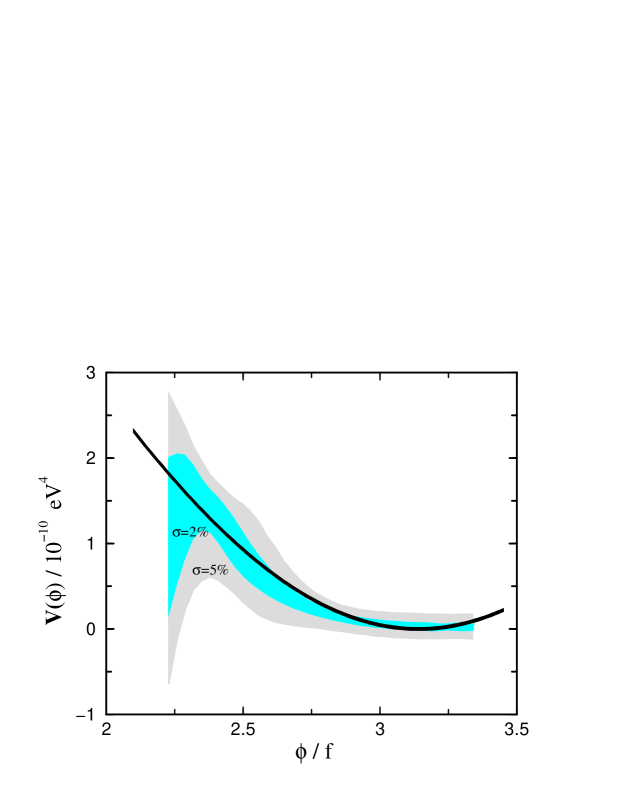
Figure 1: The 95% confidence interval for the reconstructed potential assuming luminosity distance errors of 5% and 2% (shaded areas) and the original potential (heavy line). For this reconstruction, $\Omega_{M}=0.3$, $V(\phi)=V_{0}[1+\cos(\phi/f)]$, $V_{0}=(4.65\times 10^{-3}{\,\rm eV})^{4}$, $f/{m_{\rm Pl}}=0.154$, $N=40$, and $z_{\rm max}=1.0$. The simulated data were fit by a fourth-order polynomial in $z$.

Here we investigate the feasibility of our approach and estimate the inherent errors by means of simulated data and Monte-Carlo realization. Our procedure is straightforward:

• Pick a potential $V(\phi)$, matter density $\Omega_{M}$, and values for $\phi_{0}$ and $\dot{\phi}_{0}$ (consistent with $\Omega_{\phi}=1-\Omega_{M}$)

• Compute the evolution of $\phi$, $a(t)$ and $r(z)$ for this quintessence model by evolving $\phi(t)$ and $a(t)$ back in time

• Realize the model by simulating SNe Ia measurements: for $z_{i}=(i-1)\Delta z$ and $i=1$ to $N$, $r_{i}=r(z_{i})+\delta r_{i}$ where $\delta r_{i}$ is drawn from a Gaussian distribution with zero mean and variance $\sigma\,r_{i}(z)$ ($\sigma$ is the relative error in the luminosity distance)

• Fit the simulated data with a (low-order) polynomial and numerically compute $V(\phi)$ from the reconstruction equations

• Repeat one thousand times to estimate the error in reconstructing $V(\phi)$

• This procedure actually reconstructs $\omega(\phi)$; to get $V(\phi)$ one simply takes a value for $H_{0}$; for our results we took $H_{0}=70\,{\rm km}\,\,{\rm sec}^{-1}\,{\rm Mpc}^{-1}$

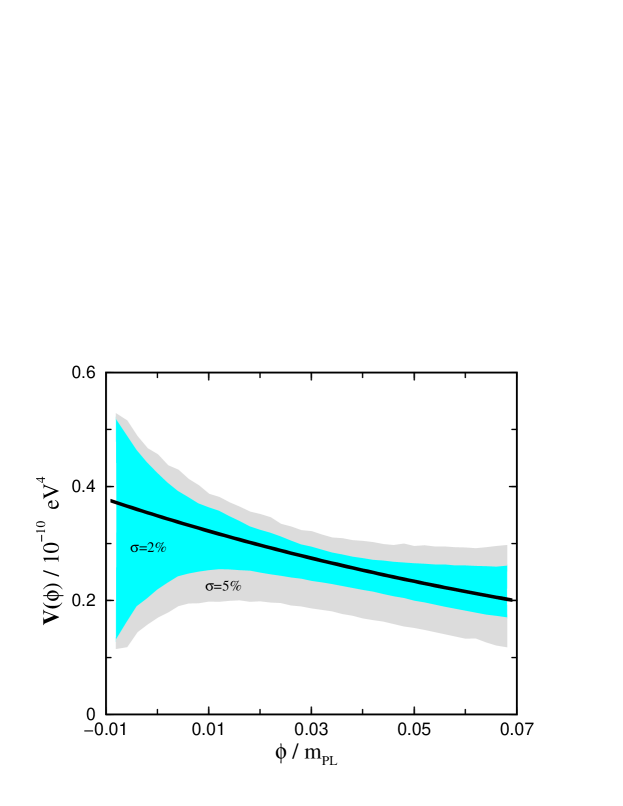
Figure 2: The 95% confidence interval for the reconstructed potential assuming luminosity distance errors of 5% and 2% (shaded areas) and the original potential (heavy line). For this reconstruction, $\Omega_{M}=0.4$, $V(\phi)=V_{0}\exp(-\beta\phi/{m_{\rm Pl}})$, $V_{0}=(2.43\times 10^{-3}{\,\rm eV})^{4}$, $\beta=8$, $N=40$, and $z_{\rm max}=1.5$. The simulated data were fit by a fourth-order polynomial in $z$.

Before presenting some results, we should elaborate on a few technical details. In fitting a polynomial to $r_{i}$ we have tried third-, fourth-, fifth-, and sixth-order polynomials; all give similar results. Because we are taking derivatives of $r(z)$, the use of higher-order polynomials only introduces numerical “noise” and is not useful. We have varied the number of redshift bins $N$ from 20 to 100, and $z_{\rm max}\equiv(N-1)\Delta z$ from 1 to 1.5; the errors in the reconstruction scale roughly as expected, $1/\sqrt{N}$. We also tried using a Gaussian distribution in redshift (with more data points at small $z$ than at high $z$); the results change little relative to the case of linear distribution.

We have reconstructed several potentials; here, we present results for the exponential and cosine potentials considered previously [4, 5]. Shown in Figs. 1 and 2 are the original potential and the 95% confidence intervals for the reconstructed potential for data with 5% and 2% luminosity distance errors. The confidence intervals are obtained by requiring that 950 of the 1000 Monte Carlo realizations give a value of the potential in that interval. The error in the reconstructed potential is mostly attributable to the $d^{2}r/dz^{2}$ terms in the reconstruction equations, reflecting the fact that it is extremely difficult to infer the second derivative of the noisy data. In particular, an uncertainty of 10% in $\Omega_{M}$ does not change the reconstruction confidence regions appreciably.

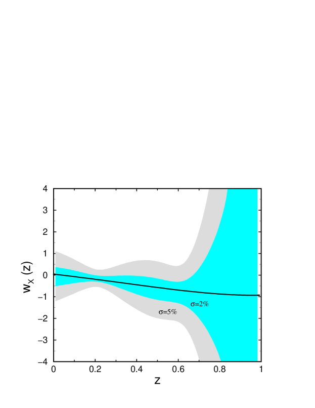
Figure 3: The 95% confidence interval for the reconstructed equation of state of the unknown component assuming luminosity distance errors of 5% and 2% (shaded areas) and the original equation of state (heavy line). For this reconstruction, $\Omega_{M}=0.4$, $V(\phi)=V_{0}\exp(-\beta\phi/{m_{\rm Pl}})$, $V_{0}=(2.43\times 10^{-3}{\,\rm eV})^{4}$, $\beta=15$, $N=40$, and $z_{\rm max}=1.0$. The simulated data were fit by a third-order polynomial in $z$.

Finally, Fig. 3 shows the reconstruction of the equation of state for an exponential potential. Even though the uncertainties in the reconstruction are large, we are still able to distinguish this quintessence model from a constant equation of state. In particular, using the $\chi^{2}$ statistic for $r(z)$ and the simulated data with 2% errors, all constant equations of state can be ruled out with 99.9% confidence, and the most plausible constant equations of state, $w_{X}=-N/3$ for $N=0,1,2,3$, can be ruled out with more than 99.9% confidence. (Of course, the ability to discriminate between constant $w_{X}$ and varying $w_{X}$ depends upon how $w_{X}$ varies.) Fig. 3 also nicely illustrates a general feature of reconstruction: Because the fractional contribution of dark energy rapidly decreases with increasing redshift, $\rho_{X}/\rho_{M}\propto(1+z)^{3w_{X}}$, reconstruction beyond redshift of around $z\sim 0.8$ becomes extremely difficult. Thus, for the purposes of reconstruction, data at redshifts greater than unity are of very limited value.

4 Discussion

If correct, the discovery that the expansion of the Universe is speeding up rather than slowing down is one of the most important discoveries of this century. It implies that the primary component of the cosmos today is dark energy with large negative pressure and of unknown composition. The implications for fundamental physics are equally profound as all the possibilities for the dark-energy component are deeply rooted in fundamental physics: vacuum energy, a frustrated network of topological defects and an evolving scalar field.

The measurement of distances to supernovae out to redshift of order unity, which led to this discovery, may also be of great utility in determining the character of the dark energy. In this paper we have derived the equations that relate the equation of state of the dark-energy component and, in the case of quintessence, the scalar-field potential to measurements of the luminosity distance. By use of Monte-Carlo simulation we have shown how this might be done in practice and addressed the feasibility of this technique.

While ours is a preliminary investigation, the results indicate that using SN Ia measurements to probe the dark-energy component is promising. However, important questions and issues remain before one can be confident that this technique can be used in practice. Some involve the technical details of how our method might be implemented: What is the optimal distribution of supernova redshifts for probing $w_{X}$ and $V(\phi)$? Would a likelihood analysis for a parameterized fit to the potential be more powerful than our reconstruction approach? We have already begun to address these questions with some success. For example, we have found that Pade approximants are a much better way to represent the observational data than polynomials (splines may do even better); for many potentials a linear distribution in redshift minimizes the area of the 95% confidence region for the reconstructed potential.

Foremost among the open issues is the reliability of SNe Ia as distance indicators. Currently, the distances errors are estimated to be of order 10% to 20% (per supernova) [12]. They arise from a variety of sources: reddening due to the host galaxy or intergalactic dust; intrinsic dispersion in the brightness – decline relationship (Phillips relation [13]) used to calibrate the SNe Ia; possible systematic (with redshift) evolutionary effects; and possible dependence upon the differing chemical composition of the supernova progenitors. There is much activity, both theoretical and observational, directed at better understanding type Ia supernovae and so we can hope for improvement in reducing and/or better understanding systematic errors. Further, if the intrinsic scatter (both statistical and systematic) in the brightnesses of SNe Ia is random (not correlated with redshift), then distance error can be beaten down by more measurements. For example, allowing 10% distance error per supernova, 3% errors in $r(z)$ could be obtained if 10 supernovae are measured at each redshift, increasing the total needed for our reconstruction method to 500 or so. Finally, the two groups have proven that discovering 1000s of SNe1a over the next decade is a very realistic goal, and with a better understanding of SNe Ia, one could cull a large sample to form a smaller, higher quality sample with smaller systematic error and statistical scatter.

To summarize, distance measurements to type Ia supernovae with redshifts less than order unity have the potential to shed light upon the nature of the dark energy. Based upon existing SNe Ia measurements and their uncertainties, it appears that obtaining data of the quantity and quality required to probe the dark-energy component using the method we have described, while not guaranteed, is also not unrealistic.

Acknowledgments.

This work was supported by the DoE (at Chicago and Fermilab) and by the NASA (at Fermilab through grant NAG 5-7092). MST thanks the Aspen Center for Physics for providing a quiet, but stimulating place to finish this work.

References

- [1] M.S. Turner, G. Steigman, and L. Krauss, Phys. Rev. Lett. 52, 2090 (1984); P.J.E. Peebles, Astrophys. J. 284, 439 (1984); L. Krauss and M.S. Turner, Gen. Rel. Grav. 27, 1137 (1995); J.P. Ostriker and P.J. Steinhardt, Nature 377, 600 (1995); A.R. Liddle et al., Mon. Not. R. astron. Soc. 282, 281 (1996).
- [2] A. Vilenkin, Phys. Rev. Lett. 53, 1016 (1984); R.L. Davis, Phys. Rev. D 35, 3705 (1987); M. Kamionkowski and N. Toumbas, Phys. Rev. Lett. 77, 587 (1996); D.N. Spergel and U.-L. Pen, Astrophys. J. 491, L67 (1997).
- [3] M. Bronstein, Physikalische Zeitschrift Sowjet Union 3, 73 (1933); M. Ozer and M.O. Taha, Nucl. Phys. B287 776 (1987); K. Freese et al., Nucl. Phys. B287 797 (1987); B. Ratra and P.J.E. Peebles, Phys. Rev. D 37, 3406 (1988).
- [4] K. Coble, S. Dodelson, and J. Frieman, Phys. Rev. D55, 1851 (1996); L.F. Bloomfield-Torres and I. Waga, Mon. Not. R. astron. Soc. 279, 712 (1996).
- [5] R. Caldwell, R. Dave, and P.J. Steinhardt, Phys. Rev. Lett. 80, 1582 (1998).
- [6] S. Hancock et al, Mon. Not. R. Astron. Soc., 29, L1 (1998); C. Lineweaver, Astrophys. J. 505, 69 (1998); K. Coble et al, ibid 519, L5 (1999).
- [7] A. Dekel et al, in Critical Dialogues in Cosmology, edited by N. Turok (World Scientific, Singapore, 1997), p.175; M.S. Turner, astro-ph/9901109 (Physica Scripta, in press).
- [8] S. Perlmutter et al, astro-ph/9812133. A. Riess et al, Astron. J., 116, 1009 (1998).
- [9] P.M. Garnavich et al, Astrophys. J. 509, 74 (1998).
- [10] M.S. Turner and M. White, Phys. Rev. D 56, R4439 (1997).
- [11] S. Perlmutter, M.S. Turner and M. White, Phys. Rev. Lett., in press (1999) (astro-ph/9901052).
- [12] B. Schmidt et al, Astrophys. J. 507, 46 (1998).
- [13] M. Phillips, Astrophys. J. 413, 108 (1993).