Abstract

I discuss the evolution of the redshift-space bispectrum via perturbation theory (PT) and large high-resolution numerical simulations. At large scales, we give the multipole expansion of the bispectrum in PT, which provides a natural way to break the degeneracy between bias and $\Omega$ present in measurements of the power spectrum distortions. At intermediate scales, we propose a simple phenomenological model to take into account non-linear effects. N-body results show that at small scales the perturbative shape of the bispectrum monopole in redshift-space is preserved, breaking the hierarchical form valid in the absence of distortions.

Redshift Distortions: Perturbative and N-body Results

CITA, McLennan Physical Labs, 60 St George, Toronto, ON M5S 3H8, Canada

1 Introduction and PT Results

The bispectrum, the three-point function of density fluctuations in Fourier space, is the lowest order statistic that carries information about the spatial coherence of large-scale structures. Non-linear perturbation theory predicts a characteristic dependence of the bispectrum on the shape of the triangle, which provides a signature of gravitational instability that can be used to probe the gaussianity of initial conditions and the bias of the galaxy distribution [2]. However, in order to use it in redshift surveys, redshift distortions due to peculiar velocities must be taken into account. In this talk, I discuss the evolution of the redshift-space bispectrum in PT and N-body simulations [7].

In the plane-parallel approximation, where the observed position ${\bf s}$ of a galaxy is given by ${\bf s}={\hbox{\BF x}}-f\ {\hbox{$u_{z}$}}({\hbox{\BF x}}){\hat{z}}$, with ${\hat{z}}$ a fixed direction, $f(\Omega)\approx\Omega^{0.6}$, and ${\bf u}({\hbox{\BF x}})\equiv-{\hbox{\BF v}}({\hbox{\BF x}})/({\cal H}f)$, with ${\hbox{\BF v}}({\hbox{\BF x}})$ the peculiar velocity field; the density contrast in redshift-space reads [7]

$$\delta_{s}({\hbox{\BF k}})=\int\frac{d^{3}x}{(2\pi)^{3}}\ {\rm e}^{-i{\hbox{\BF k}}\cdot{\hbox{\BF x}}}\ {\rm e}^{ifk_{z}{\hbox{$u_{z}$}}({\hbox{\BF x}})}\ \Big{[}\delta({\hbox{\BF x}})+f\nabla_{z}{\hbox{$u_{z}$}}({\hbox{\BF x}})\Big{]}.$$ (1)

This equation describes the full non-linear density field in redshift-space in the plane-parallel approximation, and is the starting point for the perturbative approach in redshift-space. The term in square brackets describes the “squashing effect”, i.e. the increase in clustering amplitudes due to infall, and gives the standard Kaiser formula in linear PT [5]. The exponential factor encodes the “fingers of god” (FOG) effect, which erases power due to velocity dispersion along the line of sight. From Eq. (1), it is straightforward to obtain the density field to any order in PT; in particular, the hierarchical amplitude $Q_{s}$ follows from second-order PT [4]

$$Q_{s}({\hbox{\BF k}}_{1},{\hbox{\BF k}}_{2},{\hbox{\BF k}}_{3})\equiv\frac{B_{s}({\hbox{\BF k}}_{1},{\hbox{\BF k}}_{2},{\hbox{\BF k}}_{3})}{[P_{g}^{0}(k_{1})\ P_{g}^{0}(k_{2})+P_{g}^{0}(k_{2})\ P_{g}^{0}(k_{3})+P_{g}^{0}(k_{3})\ P_{g}^{0}(k_{1})]}$$ (2)

where the $B_{s}$ denotes the bispectrum and $P_{g}^{0}(k)\equiv b^{2}(1+\frac{2}{3}\beta+\frac{1}{5}\beta^{2})P(k)$ is the power spectrum monopole of galaxies in linear PT assuming deterministic biasing, and $\beta\equiv f/b$. Decomposing into multipoles with respect to $\mu$, where $\mu\equiv\hat{{\hbox{\BF k}}}_{1}\cdot\hat{z}$, we obtain the tree-level monopole of the equilateral hierarchical amplitude [7]:

$$Q_{s\ {\rm eq}}^{(\ell=0)}=5\ A(\gamma,\beta,b)\ /[98\,b\,(15+10\,\beta+3\,\beta^{2})^{2}],$$ (3)

where $A\equiv 2520+4410\gamma+3360\beta+2940\gamma\beta+1260\beta^{2}+441\gamma\beta^{2}+72\beta^{3}-63b\beta^{3}-14b\beta^{4}$, $\gamma\equiv b_{2}/b$, and $b_{2}$ is the non-linear bias. For no biasing this yields $Q_{s\ {\rm eq}}^{(0)}=0.464$ for $\Omega=1$. The quadrupole to monopole ratio of $B_{\rm eq}$ is

$$R_{\rm B}=[5/(22A)](7392\beta+6468\gamma\beta+3960\beta^{2}+1386\gamma\beta^{2}+264\beta^{3}-231b\beta^{3}-56b\beta^{4}),$$ (4)

which for no biasing gives $R_{\rm B}=11329/31394=0.36$ for $f=1$. Note that Eqs. (3-4) give a constraint on $(b,\beta,\gamma)$ that is independent of the power spectrum. These, together with $R_{P}$, the power spectrum quadrupole to monopole ratio statistic [3, 1], can be inverted to obtain $\Omega$, $b$ and $b_{2}$ at large scales, independent of the initial conditions.

2 Non-Linear Redshift Distortions and N-Body Results

In order to describe the non-linear behavior of the redshift-space bispectrum, we introduce a phenomenological model to take into account the effects of velocity dispersion . For the power spectrum, we take [6]

$$P_{s}({\hbox{\BF k}})=b^{2}\ P(k)\ (1+\beta\mu^{2})^{2}\ /[1+(k\mu\sigma_{v})^{2}/2]^{2},$$ (5)

where $\sigma_{v}$ is a free parameter that characterizes the velocity dispersion along the line of sight. It is straightforward to obtain the multipole moments of $P_{s}({\hbox{\BF k}})$ in this simple model. Here we use the quadrupole to monopole ratio statistic, $R_{P}$, to fit $\sigma_{v}$, and then propose a similar ansatz to take into account non-linear distortions of the bispectrum:

$$B_{s}({\hbox{\BF k}}_{1},{\hbox{\BF k}}_{2},{\hbox{\BF k}}_{3})=B_{s}^{\rm PT}({\hbox{\BF k}}_{1},{\hbox{\BF k}}_{2},{\hbox{\BF k}}_{3})\ /\big{[}1+\alpha^{2}\ [(k_{1}\mu_{1})^{2}+(k_{2}\mu_{2})^{2}+(k_{3}\mu_{3})^{2}]^{2}\sigma_{v}^{2}/2\big{]}^{2},$$ (6)

where $B_{s}^{\rm PT}({\hbox{\BF k}}_{1},{\hbox{\BF k}}_{2},{\hbox{\BF k}}_{3})$ is the tree-level redshift-space bispectrum. Note that we introduced a constant $\alpha$ which reflects the configuration dependence of the triplet velocity dispersion. At $z=0$, we take $\alpha\simeq 2$ for equilateral configurations, and $\alpha\simeq 3$ for $k_{1}/k_{2}=2$ configurations, independent of cosmology.

Figure 1 shows the results from this modeling and how it compares with N-body simulations, corresponding to $256^{3}$ particles in a 240$h^{-1}$ Mpc box run by the Virgo Consortium. For the SCDM model, from $R_{\rm P}$ we obtain $\sigma_{v}=6$ (in units of H₀=100 $h$ km/s/Mpc) for $z=0$ and $\sigma_{v}=2$ for z=1 (with $\alpha=1$). Using this we can predict $R_{\rm B}$ by taking multipoles in Eq. (6), the resulting $R_{\rm B}$ is shown as solid lines in Fig. 2, which despicts excellent agreement with the N-body simulation results. Similarly, for the $\Lambda$CDM model we obtain from fitting $R_{\rm P}$, $\sigma_{v}=5.5$ for $z=0$ and $\sigma_{v}=4$ for $z=1$ (with $\alpha=1.75$). The results for $R_{\rm B}$ are also in very good agreement with numerical simulations.

The bottom panels in Fig. 1 show a comparison of simulations to the predictions of PT and the model of Eq. (6) in $k_{2}/k_{1}=2$ configurations, for three different scales. We see in these panels that even though the tree-level PT prediction in real space (dotted) works reasonably well, the redshift-space counterpart (dashed) does not. On the other hand, the model in Eq. (6) (solid) describes the N-body results very well. Even at the largest scale we probed, corresponding to a wavelength $\lambda\simeq 50$ Mpc/$h$, the tree-level PT prediction in redshift-space would predict an effective bias $b=1.4$, a quite significant discrepancy. This situation is similar to what happens with the power spectrum, redshift-space statistics are more affected by non-linearities than their real-space counterparts. In this respect, it is interesting to note that even in the linear dynamics, the exponential factor in Eq. (1) can lead to a FOG effect at large scales that eventually makes $R_{\rm P}$ and $R_{\rm B}$ to become negative [7]. Therefore, the long range of the FOG effect seen in numerical simulations, should not be exclusively attributed to virialized clusters. These results strongly suggest the possibility of extending the leading-order PT results for the power spectrum and bispectrum to smaller scales by treating the redshift-space mapping in Eq. (1) exactly and approximating the dynamics using PT [7]. The bottom right panel in Fig. 1 nicely illustrates the effect of cluster velocity dispersion on redshift-space correlations in the non-linear regime, whereas $Q$ is very close to hierarchical, $Q_{s}$ has a strong configuration dependence. Eq. (6) (solid) does an excellent job in predicting $Q_{s}$, even at this considerable stage of non-linearity.

Acknowledgements.  This material is based on a paper in collaboration with H. Couchman and J. Frieman [7]. The N-body simulations were carried out by the Virgo Supercomputing Consortium (http://star-www.dur.ac.uk/ frazerp/virgo/virgo.html) using computers based at the Max Plank Institut fur Astrophysik, Garching and the Edinburgh Parallel Computing Centre.

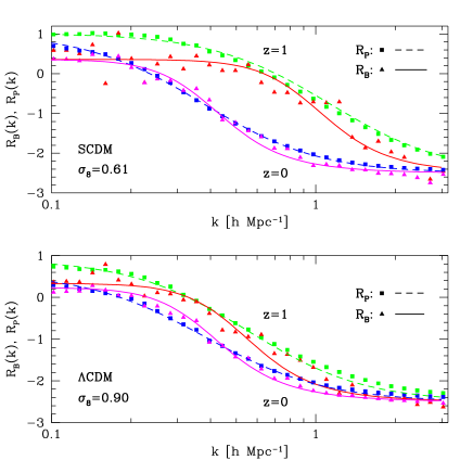
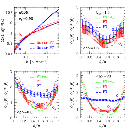
Figure 1: The top two panels show the quadrupole to monopole ratios $R_{\rm P}$ and $R_{\rm B}$ in SCDM (top) and $\Lambda$CDM simulations. The full lines show the predictions of PT convolved with an exponential velocity dispersion model, Eqs. (5-6). The bottom four panels show the power spectrum and the hierarchical amplitude $Q$ in real (squares) and redshift (triangles) space for $k_{2}/k_{1}$ configurations as a function of the angle $\theta$ between ${\hbox{\BF k}}_{1}$ and ${\hbox{\BF k}}_{2}$ for three different scales.

References

- [1] Cole, S., Fisher, K. B., & Weinberg, D. 1994, MNRAS, 267, 785
- [2] Fry, J. N. 1994, Phys. Rev. Lett., 73, 215
- [3] Hamilton, A. J. S. 1992, ApJ , 385, L5
- [4] Hivon, E., Bouchet, F. R., Colombi, S., & Juszkiewicz, R. 1995, A&A, 298, 643
- [5] Kaiser, N. 1987, MNRAS, 227, 1
- [6] Park, C., Vogeley, M. S., Geller, M. J., & Huchra, J. P. 1994, ApJ 431, 569
- [7] Scoccimarro R., Couchman, H. M. P., & Frieman, J. 1998, in preparation