A low frequency radio telescope at Mauritius for a Southern sky survey

Abstract

A new, meter-wave radio telescope has been built in the North-East of Mauritius, an island in the Indian ocean, at a latitude of $-20.14^{\circ}$. The Mauritius Radio Telescope (MRT) is a Fourier Synthesis T-shaped array, consisting of a 2048 m long East-West arm and a 880 m long South arm. In the East-West arm 1024 fixed helices are arranged in 32 groups and in the South arm 16 trolleys, with four helices on each, which move on a rail are used. A 512 channel digital complex correlation receiver is used to measure the visibility function. At least 60 days of observing are required for obtaining the visibilities up to 880 m spacing. The Fourier transform of the calibrated visibilities produces a map of the area of the sky under observation with a synthesized beam width $4^{\prime}\times 4.6^{\prime}$ sec$(\delta+20.14^{\circ})$ at 151.5 MHz.

The primary objective of the telescope is to produce a sky survey in the declination range $-70^{\circ}$ to $-10^{\circ}$ with a point source sensitivity of about 200 mJy ($3\sigma$ level). This will be the southern sky equivalent of the Cambridge 6C survey. In this paper we describe the telescope, discuss the array design and the calibration techniques used, and present a map made using the telescope.

PLATE I. An Aerial view of the Mauritius Radio Telescope. The observatory building is also seen.

PLATE II. A closer view of the helices used.

1 Introduction

Surveying the sky and compiling catalogs of celestial objects has been a major part of astronomical research for centuries. The first systematic survey of the radio universe was carried out by Grote Reber [11] using a backyard telescope with a resolution of 12^∘ operating at a frequency of 160 MHz. With the quest for higher angular resolution the exercise of surveying soon shifted to higher frequencies. Even so, many low frequency surveys were carried out after Reber’s survey some of which are summarized in Table 1. The table clearly indicates that the sixth Cambridge survey (6C) [1] is by far the most extensive survey at low frequencies. This survey provides a moderately deep radio catalog reaching a source density of about $2\times 10^{4}~{}{\rm\ sr}^{-1}$ over most of the sky north of $\delta=+30^{\circ}$ with an angular resolution of $4.2^{\prime}\times 4.2^{\prime}$ cosec$(\delta)$ and a limiting flux density of 120 mJy at 151 MHz. An equivalent of the 6C survey for the southern sky does not exist.

Since the survey of Mills et al. [9] at 80 MHz there has not been much effort at low frequencies to map the southern sky apart from the Parkes 408 MHz survey. The Culgoora [13] observations at 80 and 160 MHz were made mainly to study known sources and determine their spectral indices. The largest existing radio survey of the southern sky is the Parkes-MIT-NRAO survey [7] at 5 GHz. There is an obvious need to survey the southern sky at a frequency around 150 MHz. At this frequency synchrotron sources show up much better than at higher frequencies, such as 408 MHz, due to their spectra. Sources also show up better at 150 MHz than at lower frequencies since the absorption due to the interstellar gas is much less than at deca-meter wavelengths. For this purpose a radio telescope operating at 150 MHz has been constructed at Bras d’Eau, Mauritius.

Northern declination surveys
Freq.	Observatory	Resol.	Dec. Coverage	Sensit.	No. of Sources
408 MHz	Effelsberg	$0.85^{\circ}\times 0.85^{\circ}$	$-10^{\circ}+50^{\circ}$	0.2 Jy	–
178 MHz	Cambr. 3CR	$2^{\prime}\times 2^{\prime}$	$-5^{\circ}+90^{\circ}$	9 Jy	$328$
178 MHz	Cambr. 4C	$7.5^{\prime}\times 7.5^{\prime}$	$-7^{\circ}+80^{\circ}$	2 Jy	$4843$
38 MHz	Cambr. WKB	$45^{\prime}\times 45^{\prime}$	$-45^{\circ}+35^{\circ}$	14 Jy	$1000$
34.5 MHz	GEE TEE	$30^{\prime}\times 30^{\prime}$	$-30^{\circ}+60^{\circ}$	5 Jy	$\approx 3000$
151 MHz	Cambr. 6C	$4^{\prime}\times 4^{\prime}$	$+30^{\circ}+90^{\circ}$	0.12 Jy	$>10^{5}$
Southern declination surveys
38 MHz	Cambr. WKB	$45^{\prime}\times 45^{\prime}$	$-45^{\circ}+35^{\circ}$	14 Jy	$1000$
34.5 MHz	GEE TEE	$30^{\prime}\times 30^{\prime}$	$-30^{\circ}+60^{\circ}$	5 Jy	$\approx 3000$
408 MHz	Parkes	$0.85^{\circ}\times 0.85^{\circ}$	$-60^{\circ}+10^{\circ}$	1 Jy	–
408 MHz	Molongolo	$2^{\prime}\times 2^{\prime}$	$-60^{\circ}+18^{\circ}$	0.6 Jy	$>12000$
843 MHz	MOST	$0.4^{\prime}\times 0.4^{\prime}$	$-90^{\circ}-30^{\circ}$	–	ongoing
151.5 MHz	MRT	$4^{\prime}\times 4^{\prime}$	$-70^{\circ}-10^{\circ}$	0.2 Jy	ongoing

Table 1: Surveys below 1 GHz

The Mauritius Radio-Telescope (MRT) has been constructed and is operated collaboratively by the Raman Research Institute, the Indian Institute of Astrophysics and the University of Mauritius. It is situated in the North-East of Mauritius (Latitude 20.14^∘ South, Longitude 57.74^∘ East), an island in the Indian Ocean. It is a T-shaped array with an East-West (EW) arm of length 2048 m having 1024 helical antennas and a South (S) arm of length 880 m consisting of a rail line on which 16 movable trolleys each with four helical antennas are placed (Figure 1).

Figure 1: A schematic of the array. The EW arm has 1024 helices which are divided in 32 groups of 32 helices each. The NS arm has 16 trolleys each with 4 helices.

The helical antennas respond to frequencies between 80 and 160 MHz. Presently the telescope is operated at 151.5 MHz which allows maximum interference-free observations. The helices are mounted with a tilt of $20^{\circ}$ towards the south so that they point towards a declination of $-40^{\circ}$ at the meridian. The declination coverage corresponding to the Half Power Beam Width (HPBW) of the helices is from $-70^{\circ}$ to $-10^{\circ}$. Plate I shows an aerial view of the telescope and Plate II shows a closer view of the helices used.

The EW arm is divided into 32 groups of 32 helices each. All the EW groups are not at the same height, a situation imposed by the uneven terrain. Each trolley in the S arm constitutes one S group. Both EW and S group outputs are heterodyned to an intermediate frequency (IF) of 30 MHz, using a local oscillator (LO) at 121.6 MHz. The 48 group outputs are then amplified and brought separately to the observatory building via coaxial cables. In the observatory, the 48 group outputs are further amplified and down converted to a second IF of 10.1 MHz. The 32 EW and 16 S group outputs are fed into a $32\times 16$ complex, 2-bit 3-level digital correlator sampling at 12 MHz. The 512 complex visibilities are integrated and recorded at intervals of 1 second. At the end of 24 hours of observation the trolleys are moved to a different position and new visibilities are recorded. A minimum of 60 days of observing are needed to obtain the visibilities up to the 880 m spacing.

The Fourier transform of the phase corrected visibilities obtained after the complete observing schedule produces a map of the area of the sky under observation with a synthesized beam width of $4^{\prime}\times 4.6^{\prime}$ $\sec(\delta+20.14^{\circ})$. The phase corrections mentioned above take into consideration the non-coplanarity of the baselines. The expected root mean squared (RMS) values of the background in the synthesized images, arising from the system noise with a 1 MHz bandwidth and an integration time of 8 seconds and from the confusion noise are expected to be around 200 mJy(3$\sigma$) and 10 mJy respectively.

Table 2 summarizes the MRT specifications.

Observing frequency	151.5 MHz
Telescope configuration	T shaped 2048 m EW arm and 880 m NS arm
Basic element	helical antenna
Polarization	Right Circular
HPBW of helix	$60^{\circ}\times 60^{\circ}$
Declination coverage	-70∘ to -10∘
Collecting area of helix	4 m2 at 150 MHz
East-West arm	32 groups with 32 helices each
North-South arm	15 trolleys each with 4 helices
$1^{st}$ IF frequency	30 MHz
$2^{nd}$ IF frequency	10.1 MHz
Instrumental bandwidths	0.15,1.0,1.5,3.0 MHz
Digitization before correlation	2-bit 3-level
Correlation receiver	32 $\times$ 16 complex channels
No of baselines measured per day	$32\times 16$
Minimum and maximum baselines	0, 1024 $\lambda$
Time to get full resolution image	60 days
Synthesized beam-width	$4^{\prime}\times 4.6^{\prime}$sec$(\delta+20.14^{\circ})$
Point source sensitivity	200 mJy (3 $\sigma$)

Table 2: MRT Specifications

2 The Telescope

2.1 Design criteria

The array was designed by considering, the availability of the 512 channel Clark Lake correlator system[5], the constraints due to the available terrain and the presence of man-made interference.

Configuration

A T-shaped configuration was chosen for its simplicity. Aperture synthesis with fixed antennas in the EW arm and movable elements (trolleys) in the S arm were chosen to minimize the hardware required. An abandoned old railway line running North-South was rebuilt for use as the South arm. This new rail line, slopes downwards at about $1/2^{\circ}$ to the horizontal till about 655 m, and then slopes upwards at about $1^{\circ}$ to the horizontal. On this rail the trolleys cannot approach the EW arm nearer than 11 m.

To ensure that the array responds to structures of all sizes in the sky, the array should provide all spacings available in a square aperture. To meet this requirement at MRT, a 15 m North extension with one trolley almost touching the EW arm has been built and is used to measure the low spatial frequencies. However, this trolley cannot approach the EW array nearer than 2 m. Hence baselines with 1 m spacing in the S direction are not measured. Non-zero EW baselines with zero-spacing along the S direction are obtained by multiplying the groups of the eastern arm with the output of four helices which are a part of the first group (closest to the center) of the western arm. This has the same primary beam as a trolley and ensures a weighting similar to baselines with non-zero spacing along the S direction.

Terrain

The local terrain is rocky and very uneven, especially along the EW arm with height differences of up to 35 m. To minimize the problems of non-coplanarity, it was decided to level the EW arm in multiples of 64 m (32$\lambda$) so that the antennas in each group will be at the same height. The height profile of the groups is shown in the Figure 2. For optimal use of the 512-channel complex correlation receiver, several schemes were considered before arriving at a configuration consisting of 16 movable trolleys in the NS arm and 32 groups in the EW arm. Details of these considerations are given by K. Golap [6].

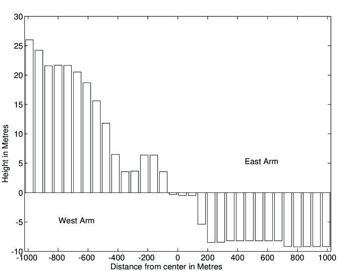
Figure 2: The EW height profile. The maximum height difference in the EW arm is 35 m.

Interference

When this telescope was conceived, man made interference in Mauritius was very low. By the time the array became operational, the increased use of many local communication networks, had increased man-made interference. The front end of the receiver system has been built with sufficient bandwidth so that the observing frequency can be shifted (within 145-155 MHz) to an interference free zone by tuning the LO. The 1 MHz band around 151.5 MHz has been found to be relatively quiet and is therefore presently being used.

2.2 The MRT Array

Helix

The primary element is a peripherally fed monofilar axial-mode helix of 3 turns with a diameter of 0.75 m and a height of 1.75 m (Figure 3). This is mounted above a stainless steel reflector mesh of grid size $2^{\prime\prime}\times 2^{\prime\prime}$. The helix is wound using a 1.5 cm diameter round aluminum tubing supported with a central UV (Ultra Violet) stabilized, light-weight PVC (Poly Vinyl Chloride) cylinder and radial PVC rods. The axial mode provides maximum radiation along the helix axis.

Figure 3: The MRT helix is a peripherally fed monofilar axial mode helix of 3 turns. The helices are mounted with a tilt of $20^{\circ}$ to allow a better coverage of the southern sky.

The helix responds to frequencies between 100 to 200 MHz with right circular polarization (IEEE definition). A quarter-wave transformer used in the feed network optimizes the VSWR to $\leq$1.5 around 150 MHz. The helical antenna, with its reflector, has a canonical collecting area of about $\lambda^{2}$ (4 m² at 150 MHz) with a HPBW of about $60^{\circ}\times 60^{\circ}$. The helices are mounted with a tilt of 20^∘ towards the South to get a better coverage of the Southern sky ($-70^{\circ}$ to $-10^{\circ}$ dec) including the Southern-most part of the Galactic plane, a region largely unexplored at meter wavelengths.

EW and S arms

The EW arm consists of 1024 helices mounted on a 2 m wide ground plane with an inter-element spacing of 2 m ($\lambda$ at 150 MHz) and is divided into 32 groups of 32 helices each.As already mentioned, due to the uneven terrain all the EW groups are not at the same height. The HPBW of the primary beam of each EW group is $1.8^{\circ}\times 60^{\circ}$ and allows observation of a source for roughly $7\times\sec(\delta)$ minutes. In each group, four helices are combined using power combiners and the combined output is pre-amplified in a low noise amplifier (noise temperature $\approx 300$K). Eight such amplified outputs are further combined and amplified to form a group output in the EW array.

Four helices mounted on a trolley with a 4 m wide ground plane constitute a group in the S array with a primary beam of HPBW $15^{\circ}\times 60^{\circ}$. Each of the 32 EW and 16 S group outputs are heterodyned to an IF of 30 MHz, amplified and transmitted, using coaxial cables, to the observatory building situated close to the center of the array. Equal lengths of coaxial cables are used irrespective of the distance of the groups from the observatory to ensure that the interferometer outputs are not affected much by changes in the ambient temperature. The configuration of the EW group is shown in Figure 4. Each NS trolley has a similar signal flow path except that there are only 4 helices and 1 pre-filter unit.

Figure 4: Signal path of an EW group. The NS trolley has a similar flow path except that there are only 4 helices and 1 pre-filter unit

Local Oscillator System

Low loss (2.4 dB /100 m at 120 MHz) heliax cables running parallel to the East, West and South arms of the array are used to distribute the LO signal required for heterodyning. The 121.6 MHz LO signal at each group is obtained by using directional couplers. To maintain a more or less constant power level for the LO signal ($-5$ dBm to $-7$ dBm) across the array, broad-band high-power amplifiers are placed at several places along the heliax cable.

To minimize the spurious correlations in the visibility measurements, the following hardware features are built into the LO system.

• The first LO is phase switched to minimize the effects of cross coupling. The Clark Lake correlator has the facility for generating the Walsh functions required for switching. But it is not practical to use many independent switching waveforms in a series fed LO system owing to the problem of distribution. Hence, we use a simple arrangement in which the LO to the first eight southern groups remain unswitched while, the eastern, the western and the remaining southern groups are switched with orthogonal square waves. The disadvantage of this scheme is that the products of the outputs from groups having same switching signal are prone to spurious correlations (eg. the product of any two eastern arm group outputs).

• The signal generator used to produce the LO also generates spurious signals at other frequencies. The spurious signals around 30 MHz, which is our First IF frequency, leaks to the IF port from the LO port of the mixer and results in correlation several times the detection limit. This is minimized by using a band rejection device centered around 30 MHz in the LO path. Band rejection is achieved using a band-pass filter centered around 30 MHz and a power-splitter (Figure 4). The filter absorbs the signal around 30 MHz and reflects the LO required for heterodyning.

2.3 The Receiver System

2.3.1 Second IF and correlator modules

In the observatory building the 48 group outputs are further amplified. Each of the 32 EW group outputs are split into two using power dividers. One set of the outputs are combined to form a fan beam of $4^{\prime}\times 60^{\circ}$ using phase-shifter modules. This single beam forming receiver provides a two degree tracking system. Details of Pulsar observations carried out using this system are described by N. Issur [8].

The second set of 32 EW group outputs and the 16 S outputs are down converted to 10.1 MHz (second IF). Four IF bandwidths, ranging from 0.15 to 3 MHz are selectable. Signals are then fed to an Automatic Gain Control (AGC) module which keeps the output power level constant. Each of the 16 group outputs of the S arm and the 16 group outputs of the E arm is split in a quadrature hybrid to obtain the in-phase and quadrature components. Then the signals are digitized to 2-bit 3-level, sampled at 12 MHz and fed into the 32 $\times$ 16 complex correlator to obtain the EW $\times$ S outputs. The high sampling rate is to reduce the loss of sensitivity due to quantization. More details of the system are given by Erickson et al.[5]. Figure 5 shows the general layout of the samplers, delay lines and correlators.

Figure 5: Diagram showing the general layout of the signals to the correlators

The last group of the East array (E16) is fed to the correlator in the place of the $16^{\rm th}$ trolley. This gives a set of baselines formed between E16 and the E-W array on all observing days. This helps to check the repeatability of data. These baselines with each trolley give 31 independent closure information which are used in the calibration. This mode of observing reduces the number of usable trolleys to only 15.

Many observing programs require the formation of fan beams [8] corresponding to each arm of the array. The correlator can also be configured to obtain E $\times$ EW and S $\times$ S correlations.

Self-correlators

Sixty four self-correlators are available in the receiver system. This provides the necessary information for obtaining the normalized correlation coefficient from the measured digital correlation counts using the correction given by D’Addario et al.[3].

$$\rho=\gamma-\frac{\gamma^{3}(\alpha_{1}^{2}-1)(\alpha_{2}^{2}-1)}{6}$$ (1)

where $\gamma=(\pi/2)(N/N_{max})\exp{(\alpha_{1}^{2}+\alpha_{2}^{2})/2}$. $\alpha_{1}$ and $\alpha_{2}$ are the $V_{th}/\sigma$ of the two channels being correlated and $N/N_{max}$ is the ratio of the correlation value to the maximum value possible out of the 2-bit 3-level system ($V_{th}$ is the threshold voltage for digitization and $\sigma$ is RMS value of the signal fed to the digitizer).

The AGCs maintain a constant power level to the samplers, even though the brightness distribution of the sky changes. Therefore we do not get the amplitude information of the signal from the sky. This results in identical correlation for a weak source in a weak background and a stronger source in a correspondingly stronger background. To measure the absolute brightness while using the AGC there is a need to measure the gains. In many telescopes this is done by adding a fixed amount of a known signal at each antenna. At the MRT, however, the variation in the background radiation as seen by the EW and the S groups are measured separately by switching off the AGCs, one in each of the EW and the S arms and using the self-correlators to measure the total power output of these groups.

The self correlators of the MRT are wired such that they measure the probability ($P$) that the input signal amplitude, $V$, is between the threshold levels used for digitization. This probability for a zero-mean Gaussian signal with RMS fluctuation of $\sigma$ and a symmetric 2-level digitizer with voltage threshold levels $\pm V_{th}$, is given by

$$P=\frac{1}{\sigma\sqrt{2\pi}}\int_{-V_{th}}^{+V_{th}}e^{-(\frac{V}{\sqrt{2}\sigma})^{2}}dV=erf(\frac{V_{th}}{\sqrt{2}\sigma})$$ (2)

knowing $P$, the RMS fluctuation $\sigma$ of the signal can be obtained. The analog correlation $\rho_{a}$ is obtained using the relation

$$\rho_{a}=\rho\times\sigma_{1}\times\sigma_{2}$$ (3)

where $\sigma_{1}$ and $\sigma_{2}$ are the RMS of the signals correlated.

In a 2-bit 3-level correlator, sampling the digitized signal at Nyquist rate, the maximum sensitivity obtainable relative to an analog correlator is 0.81. This is obtained when $V_{th}/\sigma$ is 0.61. The sensitivity changes by only 5% from this optimal value when the signal power changes by 40% [2]. Hence, switching off the AGC does not affect the signal-to-noise ratio (SNR) of the channels used to measure the total power as the variation of the sky brightness is less than $40\%$.

Recirculator

Although the use of larger bandwidths results in better sensitivity of a telescope, it restricts the angular range over which an image can be made if the relative delays between the signals being correlated are not compensated. When the uncompensated delay between the signals becomes comparable to the inverse of the bandwidth used, the signals will be decorrelated. At MRT we normally use a bandwidth of 1 MHz. Since the EW group has a narrow primary beam of two degrees in RA, this bandwidth does not pose a problem for synthesizing the primary beam in this direction. However both the EW and NS groups have wide primary beams in declination extending from $-70^{\circ}$ to $-10^{\circ}$. For signals arriving from zenith angles greater than 10 degrees on NS baselines longer than 175 m, the uncompensated delay results in bandwidth decorrelation greater than 20%.

To overcome this loss of signal one has to measure visibilities with appropriate delay settings, while imaging different declination regions. To keep the loss of signal for a bandwidth of 1 MHz to less than 15% in the entire declination range $-70^{\circ}$ to $-10^{\circ}$, the longer baselines have to be measured with four delay settings.

With the existing correlator system this implied observations for four days at trolley locations measuring long baselines. Furthermore, to be able to make interference free maps, observations have to be repeated approximately 3 times at each location. This would make the time required to complete the survey very large.

To solve this problem, a recirculator system which measures visibilities with different delay settings using the available correlators in a time multiplexed mode has been incorporated in the receiver system[12]. In this system, the data is sampled at 3 MHz, stored in a buffer memory and the correlations are measured at 12 MHz rate. Such processing by the correlator at a higher speed than the input sampling rate allows correlations to be measured with four delay settings. This ensures that the observations at each trolley allocation, even at longer baselines, can be carried out in one day, thereby, improving the surveying sensitivity. The loss of sensitivity due to the decrease in the input sampling rate from 12 MHz to 3 MHz is not serious. The recirculator system is described in detail by S. Sachdev [12].

The recirculator system can configure the correlator in the $(E+W)\times E$ and $S\times S$ modes for one integration time (roughly 100 ms in every second of data collection). Since both EW and S arrays are linear, this mode provides visibilities on several redundant baselines to calibrate the array using the Redundant Baseline Calibration technique [10]. Presently the software at MRT does not make use of this data for array calibration.

2.4 Observations

In the T configuration, we are interested in sampling baselines with north-south components from 0 m to 880 m with a sampling of 1 m (except the 1 m spacing [Section 2.1]). This ensures that the grating response will be confined well outside the primary beam response. To measure the visibilities with a 1 m spacing using 15 trolleys however requires 60 days of observing. Each day the trolleys are spread over 84 m with an inter-trolley spacing of 6 m. 512 complex visibilities are recorded with 1 sec of integration. After obtaining data for 24 sidereal-hours the trolleys are moved by one meter. After 6 days of successful observing we get visibilities measured over 90 m. The trolleys are then moved en bloc to measure the next set of visibilities.

3 Imaging with the MRT

The visibilities measured are processed off-line using MARMOSAT, the MAuRitius Minimum Operating System for Array Telescopes[4]. This is designed in-house to transfer the visibilities to images which can be ported to AIPS. The flow diagram showing the various processing stages is shown in Figure 6.

Figure 6: Flow Diagram of data acquisition, checking and processing.

The programs in MARMOSAT cater to the following needs: detection of bad data, determination of complex gain of the antennae, position calibration of antennas, combining data of different days, transforming the visibilities to get brightness distribution.

The program Online presents an uncalibrated view of the data. It is designed to read visibilities from several baselines and offers to display many functions such as phase, magnitude, closure and fringe frequencies of the visibility measured. The program Health monitors the signal-to-noise ratio of the visibilities, correlator offsets, magnitudes of the visibility of all the baselines and displays the mean and the scatter. This helps to detect gross errors quickly. The program Interference Detection detects the interference points which are rejected in subsequent processing. The details of interference detection and their statistics at MRT are given by S. Sachdev[12]. The programs Fringe-cal and the Transform are very special to the MRT due to its non-coplanarity and configuration. The following sections describe the concepts behind these programs. Further details of these programs are given by R. Dodson[4].

3.1 Antenna calibration

The complex gains of the 47 antennas are estimated using the measured visibilities for the calibrators MRC0915-119, MRC1932-464 and MRC2211-173. The sensitivity per baseline is 30 Jy for an integration time of one second. In the $1.8^{\circ}$ EW-group primary beam, the above sources are observable in each baseline with a minimum SNR of about 35.

One of the advantages of observing in the Southern sky is that the two very strong sources, Cyg A and Cas A are not in the primary beam, where they would dominate the system temperature causing dynamic range problems.

The disadvantage, however, is a paucity of strong sources required for reliable calibration. This leaves us with a situation where we can calibrate the array only a few times in a sidereal day.

The visibility phase is estimated by fringe fitting (hence the name Fringe-cal for the program), where we assume that the sky in the primary beam is dominated by the calibrator. The instrumental phase estimated is simply the difference between the phase of the observed visibilities and the expected geometric phase due to the point source calibrator (or calibrators). The instrumental gain is estimated by measuring the relative amplitudes of the fringes on different baselines. The instrumental phase is insensitive to short term interference and also to fringes due to other sources in the sky, provided their fringe rate is significantly different from that of the calibrator for a given baseline. Therefore, at short baselines where there are less than two fringes in the EW-group beam due to the calibrator, satisfactory calibration cannot be obtained.

This is tackled at MRT by calculating 47 antenna complex gains from the measured 512 complex visibilities (base2antenna in Figure 6). At this stage we reject those baselines with short EW components (essentially the first four E and W group outputs with the S array) and input the closure information obtained from multiplying the E16 group with the EW and S array group outputs.

We have found that the day-to-day RMS variation per baseline in phase is about $\pm 7^{\circ}$ and the RMS amplitude variation is about $\pm 0.1$ dB. The RMS variation of phase from one calibrator to another (eg. MRC1932-464 and MRC0915-119) is about $\pm 10^{\circ}$.

Transforming Visibilities to Brightness

The u,v coverage of MRT (EW and the NS components of the baseline) can be thought of as a pleated sheet, extended in both u and v, with discrete steps in w (height) as we move from one EW group to the one at a different height. As we are imaging a very large field of view ($60^{\circ}$ field), the approximate coplanar approach, wherein the phase term due to the heights is assumed to be a constant over the synthesized field of view, is invalid. Thus for MRT, a 3D imaging method is required.

Here we transform the visibilities using a Fast Fourier Transform (FFT) along the regularly sampled v axis, apply a Direct Fourier Transform (DFT) along the w axis and finally sum along u to obtain the image on the meridian. A DFT on w is required as the sampling is not uniform. The direct transform corrects every term along the zenith angle on the meridian for the group heights. This is equivalent to phasing the groups to a common (and artificial) 2D plane.

The NS array slopes downwards at about $1/2^{\circ}$ to the horizontal till about 655 m, and then slopes upwards at about $1^{\circ}$ to the horizontal. These two parts are treated separately while transforming. The slope is taken into account by assuming an instrumental zenith appropriate to the slope of the track. While combining contributions from different parts we introduce necessary corrections to get an instrumental zenith equal to the latitude of the place.

The sampling of the visibilities on the EW grid is at intervals equal to the size of each EW group. This gives a grating response which falls on the nulls of the primary beam while synthesizing on the meridian. For synthesis away from the meridian, one of the grating response starts moving into the primary beam. This leads to the synthesized beam being a function of the hour angle. Hence to simplify matters, imaging is presently done on the meridian only.

3.2 Initial Results

One set of observations for all the 880 trolley positions have been made. Because of the presence of the Sun and the day time interference, the data set is not complete for the full RA coverage. A second set of data is being taken to cover the complete accessible sky. The observations are expected to be completed in 1998.

Figure 7: Map at 13’ x 18’ resolution of a typical region away from the galactic plane. The contours are -9 -7 -5 -4 -3 -2 -1 1 2 3 4 5 7 9 11 13 15 17 19 23 27 31 35 45 55 65 Jy/beam. The coordinates are for epoch 2000

RA	Declination	Flux Density (Jy)
01:05:26	-45:04	20
01:07:51	-42:40	6
01:08:53	-52:20	4
01:13:23	-53:23	3
01:15:29	-44:23	4
01:16:30	-47:24	15
01:16:51	-52:08	10
01:17:53	-54:39	3
01:18:54	-62:42	7
01:19:58	-53:48	3
01:21:22	-49:59	4
01:23:27	-50:42	5
01:27:15	-51:37	4
01:27:34	-61:32	9
01:27:57	-48:17	4
01:28:38	-52:58	5
01:31:24	-51:06	8
01:31:44	-61:53	12
01:33:30	-44:40	10
01:43:13	-45:27	6
01:49:04	-57:47	8
01:52:33	-55:49	4
01:54:19	-43:32	5
01:55:41	-49:05	4
01:59:30	-47:30	5

Table 3: Table giving point sources detected in the image of Figure 7, the coordinates are for epoch 2000

For imaging on the meridian with all the 880 m baselines, the point source sensitivity will be about 200 mJy(3 $\sigma$) at the peak of primary beam with 8 seconds of integration and a bandwidth of 1 MHz. The confusion limit for an instrument of resolution $4^{\prime}\times 4^{\prime}$ is about 13 mJy. For extended structures the surface brightness sensitivity is about 5 mJy/arcmin².

While the data collection is under way, we are processing the available data to make a low resolution survey of the sky. Observations up to a baseline of 178 m do not require the recirculator. We have taken this as a natural cutoff and have made low resolution images using only 8 central groups of the EW arm and trolley positions up to 178 m in the NS. A part of the survey covering the RA range 18:00 to 24:00 hrs and 00:00 to 05:00 hrs has been completed. In this paper, we present a deconvolved image, of the region extending from 0100 hrs to 0200 hrs in RA and $-62^{\circ}$ and $-42^{\circ}$ in declination, with a resolution of $13^{\prime}\times 18^{\prime}\sec(\delta+20.14^{\circ})$. MRC1932-464, with a flux density of 81 Jy/beam was used as the primary flux calibrator [6]. The expected RMS noise due to confusion and system temperature (with an integration time of 19 seconds) are expected to be 0.7 Jy. The noise seen on the map is 0.8 Jy and is very close to the expected value. More than 25 point sources in the flux density range 3 to 20 Jy can be seen in the map. Many of them have been identified with Molongolo and Culgoora sources. A comparison of the flux densities of the sources common to MRT and Culgoora lists showed that the error on the estimated flux densities is less than 25%. The vertical line at RA 01h55m and the feature at RA 01h02m, Dec $-59^{\circ}$ are due to man made interference. The image has been presented here for completeness and to illustrate the success of the methods developed for imaging. A separate paper on the low resolution survey will discuss more details such as the deconvolution procedure for a non-coplanar array like MRT, method used for detecting point sources, measurement of the zero spacing and the flux density scale used.

4 Acknowledgment

We thank V. Radhakrishnan for his interest and encouragement from the initial stages of the project. Our thanks are due to W. E. Erickson for providing the CLRO correlator to MRT. We gratefully acknowledge M. Modgekar, C.M. Ateequlla and H.A. Aswathapa from the Raman Research Institute, R. Somanah and N. Issur from the University of Mauritius and G.N. Rajashekar from the Indian Institute of Astrophysics for their efforts in this project. We thank all those from the Raman Research Institute, Indian Institute of Astrophysics, and the University of Mauritius who have contributed towards this project. ChVS thanks J. E. Baldwin for many useful discussions and suggestions.

References

- [1] J.E. Baldwin, R.C. Boysen, J.E. Hales, S.E.G. Jennings, P.C. Waggett, P.J. Warner, and D.M.A. Wilson. The 6c survey of radio sources – 1. Mon. Not. R. astr. Soc., 217:717–730, 1985.
- [2] F.K. Bowers and R.J. Klinger. Quantization noise of correlation spectrometers. Astr. Astrophys. Suppl., 15:373–380, 1974.
- [3] L.R. D’Addario, A.R. Thompson, F.R. Schwab, and J. Granlund. Complex cross correlators with 3-level quantization - design tolerances. Radio Science, 19(3):931–945, 1984.
- [4] R. Dodson. The Mauritius Radio Telescope and a Study of Selected Super Nova Remnants Associated with Pulsars. PhD thesis, University of Durham, 1997.
- [5] W.C. Erickson, M. J. Mahoney, and K. Erb. The clark lake teepee-tee telescope. Astrophys. J. Suppl., 50(403-419), 1982.
- [6] K. Golap. Synthesis Imaging at 151.5 MHz using the MRT. PhD thesis, University of Mauritius, 1998.
- [7] M.R. Griffith and A.E. Wright. Astron. J., 105:1666, 1993.
- [8] N. Issur. Pulsar observation with mrt. Bull. Astr. Soc. India, 1997.
- [9] B.Y. Mills, O.B. Slee, and E.R. Hill. A catalogue of radio sources. Aust. J. Phys., 11:360, 1958.
- [10] J. E. Noordam and A.G. de Bruyn. High dynamic range mapping of strong radio sources,with application to 3c84. Nature, 299:597, 1982.
- [11] G. Reber. Astrophys. J., 100:279, 1944.
- [12] S. Sachdev. Wide Field imaging with the Mauritius Radio Telescope(under preparation). PhD thesis, University of Mauritius, 1998.
- [13] O.B. Slee. Culgoora-3 list of radio source measurements. Aust. J. Phys. Astrophys. Suppl., 43:1–123, 1977.