Expansion of W 3(OH)

Abstract

A direct measurement of the expansion of W 3(OH) is made by comparing Very Large Array images taken $\sim 10\,\rm yr$ apart. The expansion is anisotropic with a typical speed of $\rm 3\,\,to\,\,5\,km\,s^{-1}$, indicating a dynamical age of only $2300\,\rm yr$. These observations are inconsistent with either the freely expanding shell model or a simple bow shock model. The most favored model is a slowly expanding shell-like H ii region, with either a fast rarefied flow or another less massive diffuse ionized region moving towards the observer. There is also a rapidly evolving source near the projected center of emission, perhaps related to the central star.

1 Introduction

Ultra-compact H ii (UCH ii) regions are small but dense envelopes of ionized gas that form out of the natal material around early-type massive stars that have just formed. While the general scenario of how massive stars form and how they might appear were theoretically described more than several decades ago (Davidson & Harwit 1967, Larson 1969a, b, 1972, Yorke & Krügel, 1977), the lack of observational probes have frustrated efforts to understand these regions in greater detail. One of the pressing questions raised recently regarding high-mass star formation is exactly how UCH ii regions evolve with time. Specifically, how long UCH ii regions persist is currently a puzzle.

UCH ii regions are typically under 0.1 pc in size, $\sim 10^{17}\,\rm cm$, but extremely dense, $n_{e}>10^{5}\,\rm cm^{-3}$. The high density and temperatures of $\sim 10^{4}\,\rm K$, typical of H ii regions, together suggest that there should be strong pressure imbalance between the ionized region and its surrounding medium. Massive molecular outflows are commonly observed near UCH ii regions, and highly turbulent velocities are also present in spectral line profiles. UCH ii regions are also closely associated with sites of very energetic $\rm H_{2}O$ and OH masers, indicating that there is a strong interaction between the central stars, which supply the energy for the masers, and the molecular material outside the ionized region. Massive stars are also known to possess strong stellar winds that greatly affect their environment. This combination of observational clues suggests that the ionized regions should be rapidly both evolving and expanding, provided there is no constraint to the expansion. For an unconstrained expansion the estimated age of UCH ii regions is approximately the size of the region divided by the sound crossing speed, and for most UCH ii regions the inferred age is $\sim 10^{3}$ to $10^{4}\,\rm yr$. Presumably, after this phase, most of the material that shrouds the star is blown away, revealing optically the star with its H ii region.

However, several studies of the statistics of UCH ii regions suggest that the lifetime of the ultra-compact phase is of order $10^{5}\,\rm yr$, considerably longer than the dynamical age. Nearly two decades ago, Habing & Israel (1979) recognized that the time scales of several concurrent phenomena were inconsistent with the dynamical age of UCH ii regions. The time scale for natal material to coalesce to form stars, and the time over which $\rm H_{2}O$ masers are thought to exist are both about $10^{5}\,\rm yr$. Since both processes are seen in vicinity of almost all UCH ii regions, it is unlikely that the UCH ii phase could be significantly shorter in duration than the two processes. Therefore, UCH ii regions are perhaps longer lived than suggested by the dynamical age.

More recently the analysis of Infrared Astronomy Satellite (IRAS) sources by Wood & Churchwell (1989b) showed that between perhaps 10 and 20% of all O stars are still embedded in molecular clouds. This implies that the UCH ii phase lasts for up to 20% of the lifetime of an O star or $\sim 10^{5}\,\rm yr$, in good agreement with the age predicted by Habing & Israel (1979). Probably the most convincing argument for UCH ii regions having lifetimes longer than their dynamical ages is the follow-up Very-Large-Array (VLA) survey of UCH ii regions by Wood & Churchwell (1989a). They detected a large excess in the number of UCH ii regions over that expected if the number of UCH ii regions were simply given by the total galactic O star population multiplied by the ratio of the dynamic age to the lifetime of an O star.

Thus, either UCH ii regions are presently too numerous in the Galaxy or their lifetimes are longer than expected by a factor close to $10^{2}$. Discounting the former argument, Wood & Churchwell (1989a) concluded that the UCH ii phase must persist longer than the dynamical age. This conclusion has stirred much theoretical interest and spurred many observational projects (e.g. Van Buren et al. 1990, Mac Low et al. 1990, Hollenbach et al. 1994, García & Franco 1996, Akeson & Carlstrom 1996). It is thought that either UCH ii regions are effectively and stably confined to prevent their rapid expansion, or that the observed size of the emission structure does not change because the material is constantly being replenished. The first reason may apply for some UCH ii objects with shell-like morphology, while the second may apply for others with core-halo morphology, and a combination has been suggested in a model for cometary objects as bow shocks around stars moving through molecular clouds (Van Buren et al 1990).

Clearly, one of the obstacles to understanding UCH ii regions is the lack of good observational probes. First, they are totally obscured at optical wavelengths. The central star exciting the H ii region W 3(OH) is obscured by dust with an V-magnitude extinction of $\sim 50$ (Wynn-Williams, Becklin & Neugebauer 1972). Presently, UCH ii regions can be best studied at centimeter wavelengths using synthesis imaging. Observations in the far infrared can measure the flux from the dusty cocoon that surrounds the H ii region revealing the bolometric luminosity, which indicates the star-type. Millimeter-wave interferometers do not as yet resolve the regions adequately, but should be an excellent probe of the molecular material near the H ii region if slightly higher resolutions are attained.

The compact H ii region W 3(OH) is a limb-brightened shell of dense ionized gas around an O7 star that has recently formed (Dreher & Welch 1981). Regarded as the prototypical UCH ii region, W 3(OH) is associated with a prominent cluster of OH masers (Norris & Booth 1981). The central star is totally optically obscured by an extended dusty cocoon that envelops the H ii region (Wynn-Williams et al. 1972). The H ii region is ensconced in a massive molecular cloud, $M\sim 2000\,M_{\odot}$, which extends about 1 pc across, and exists in the vicinity of two core components (Wilson, Johnston, & Mauersberger 1991). The more massive component, with mass $M\sim 60\,M_{\odot}$, is associated with the source identified by Turner & Welch (1984), which is associated with the cluster of $\rm H_{2}O$ masers about $6^{\prime\prime}$ east of the main H ii region. W 3(OH) is associated with the less massive component, with mass $M\sim 10\,M_{\odot}$. Presumably, a significant fraction of the mass in the protostellar core condensed to form the $\sim 30\,M_{\odot}$ star that excites the H ii region. The ionized region itself is a bright source at centimeter wavelengths, with a total flux of $2.2\,\rm Jy$ at 15 GHz, which is approximately the turnover frequency. The shell measures approximately $1^{\prime\prime}$ across, and for a distance of 2.2 kpc (Humphreys 1978), the H ii region is only $3\times 10^{16}\,\rm cm$ in diameter. With this flux density and dimensions for the nebula, the emission measure is in excess of $10^{9}\,\rm pc\,cm^{-6}$. The dynamical age of the H ii region, given by its diameter divided by the plasma sound speed ($c\approx 10\,\rm km\,s^{-1}$), is only $\tau_{dyn}=10^{3}\,\rm yr$.

This paper describes direct observations of the changes in the W 3(OH) region by comparing centimeter synthesis images made at several time epochs. Specifically, we exploit the proven technique of difference mapping using VLA images taken at epochs separated by several years to observe this well-studied bright UCH ii region. This robust method has been used to measure accurate distances to ionization-bounded planetary nebulae (Masson 1986). In this application the distance is measured by combining the angular expansion with spectroscopically determined velocities. In the present paper, the goal is not to measure the distance to the H ii region, but rather to use the difference maps to understand its evolution.

2 Observations

All observations were made using the NRAO VLA synthesis telescope in the A-configuration, observing in the continuum mode at 2 cm. There are three sets of observations for W 3(OH): 6 Mar 1986, 9 Mar 1990 and 25 Jun 1995. The observations are long tracks to ensure nearly complete, uniform spatial coverage of the source. Thus, the spatial coverage is similar in all epochs. Additionally, a small amount of time in the 1986 run was devoted to making 1.3 cm observations to aid in the modeling. The amplitude was calibrated with 3C 286 in the 1986 and 1990 observations, and with 3C 48 in the 1995 observations. The flux densities were assumed to be 3.49 Jy for 3C 286 and 1.81 Jy for 3C 48. For all epochs the phase calibrator was 0224+671. The 2 cm flux density for the phase calibrator 0224+671 was 0.89 Jy, 1.70 Jy, and 2.73 Jy in 1986, 1990 and 1995, respectively. To improve the sensitivity the intermediate frequency bands were averaged when appropriate. Each data set was calibrated separately in order to make independent measurements of the flux density. We estimate that the uncertainty of the amplitude of the data is 5% at 2 cm, and 10% at 1.3 cm. The flux densities and a summary of the observations are listed in Table 1. The final 1.3 cm map was made with several iterations of self-calibration and CLEAN, convolved with a $0.\kern-3.00003pt^{\prime\prime}\kern-1.00006pt1$ circular Gaussian beam. A contour map of the region is shown in Figure 1. Contour maps of the main H ii region at 15 GHz and 22 GHz are shown in Figure 2.

		No. of	Total	RMS
$\lambda$	Date	Visibilities	Flux Density	Noise
(cm)		($\times 10^{3}$)	(Jy)	($\mu\rm Jy/beam$)
2	1986 Mar 6	434	$2.23\pm 0.11$	65
	1990 Mar 9	302	$2.05\pm 0.10$	45
	1995 Jun 25	881	$2.35\pm 0.12$	40
1.3	1986 Mar 6	184	$2.8\pm 0.2$	490

Table 1: Observation Parameters

Figure 1: A contour map of the W 3(OH) region observed at 15 GHz in 1986. The main source is enclosed by the dashed box, in which the contour levels are 10% of the peak brightness, or $3.2\,\rm mJy\,beam^{-1}$. Outside the dashed box the contour levels are integer multiples of $200\,\mu\rm Jy\,beam^{-1}$. The source associated with water masers is $6^{\prime\prime}$ directly E of the main source; there is another source $8^{\prime\prime}$ to the NE.

Figure 2: Comparison of model calculations and actual maps. The bottom panels show the contour maps of W 3(OH), which, for the purposes of presentation, have been rotated by $30^{\circ}$ in position angle. The figure on the lower left is a 22 GHz map, and lower left a 15 GHz map. The top panels are contour maps of the model. Profiles of the brightness along the major and minor axes of the H ii region are also plotted in the figure. The scale is in asec.

The cross-calibrated difference mapping technique described by Masson (1986) is used to generate difference maps between epochs. In this method the data from each epoch is calibrated and imaged in the standard manner to select the epoch with the best data. The image from the best epoch is then used as the model in the cross-calibration of the data from the other epochs. This ensures that all epochs have common phase errors across the visibility plane, which would otherwise be manifest as systematic features in difference maps. This step also conveniently aligns the position of the image of subsequent subtraction. The cross-calibrated data is imaged, and its CLEAN components are subtracted from the best data set in the visibility domain. The resultant data is imaged and CLEANed. All images are then restored with the same $0.\kern-3.00003pt^{\prime\prime}\kern-1.00006pt128$ circular Gaussian beam.

The difference mapping technique is particularly suited to quantify the angular expansion of objects with sharp boundaries, such as ionization-bounded nebulae like young planetary nebulae and W 3(OH). The angular movement is calculated by either directly computing the ratio of the difference signal and the gradient of the emission, or by suitably modeling the movement. Obviously, both methods should lead to results which concur. In the case of a reasonably uniform expansion, there is little ambiguity about the meaning of the difference map measurements. The technique can also be applied to measure proper motion if there is a fiducial point source in the field.

The main difficulty in the subtraction step is the uncertainty in the source flux density. The difference maps may contain signals only a few times the map noise. For W 3(OH) this means that in order to detect a signal in the difference map, the flux must be known to about 1%. This level of accuracy in the amplitude is not readily possible with the VLA, and at 15 GHz, an uncertainty of $\sim 5\%$ is typical. A possible way to sidestep the measurement uncertainty is to assume that the flux density remains constant. This assumption, for example, is reasonable in the case of optically thin emission from a planetary nebula. In the subtraction step for W 3(OH) the total fluxes were assumed to be same for all epochs.

3 Results

Because there are three sets of observations, three difference maps were also generated. The difference maps are shown in the upper panels of Figures 3, 4 and 5, in which the difference maps are shown in contour superimposed on a grey-scale image of the region itself. Figure 3 is a difference map made from observations separated by 9.3 yr, Figure 4 by 5.3 yr, and Figure 5, by 4.0 yr. Since the difference maps were constructed by subtracting earlier from later data, the expansion is seen as an incomplete positive ring of flux surrounding a negative region. The assumption that the total flux remains constant forces the difference maps to have zero integrated flux and as a result the region inside the ring has an average negative value. Having a number of difference maps is important and convenient because it allows us to easily identify spurious signals. It is also useful to compare maps generated from observations separated by increasing time baselines to recognize and identify trends. If there are complicated difference signals, then a number of different difference maps obviously makes it easier to interpret their meaning. Most notably, in this sequence of difference maps the brightness of the ring is clearly related to the time interval between observations.

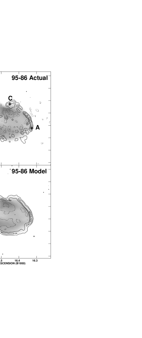
Figure 3: Difference map of W 3(OH) with a time baseline of 9.3 yr. The 15 GHz image is shown in grey scale, and the difference map is shown in contour. In the top panel the actual $95-86$ difference map is shown. A difference map generated from subtracting the 1986 image from a simulated self-similar expansion of the 1986 data is shown in the bottom panel. The frequency of the visibility was divided by a factor of 1.004, which corresponds to an expansion in the image plane. The contour levels are $200\,\mu\rm Jy\,beam^{-1}$ in both panels. Note the presense of a $-1\,\rm mJy$ signal near the center of the nebula in the upper panel.

Figure 4: Difference maps of W 3(OH) with time baseline of 5.3 yr. The 15 GHz image is shown in grey scale, and the difference map is shown in contour. In the top panel, the actual $95-90$ difference map is shown. The simulated difference maps is shown in the lower panel, in which the frequency of the visibility data was divided by a factor of 1.0023. The contour levels are $200\,\mu\rm Jy\,beam^{-1}$ in both panels.

Figure 5: Difference maps of W 3(OH) with time baseline of 4.0 yr. The 15 GHz image is shown in grey scale, and the difference map is shown in contour. In the top panel, the actual $90-86$ difference map is shown. The simulated difference maps is shown in the lower panel, in which the frequency of the visibility data was divided by a factor of 1.0017. The contour levels are $200\,\mu\rm Jy\,beam^{-1}$ in both panels. Note again the presence of the negative feature in the upper panel.

The difference maps reveal not only the expansion of W 3(OH), but also evidence of variability among other sources in the region. The first of these is located at the projected center of the main component, indicated in Figure 3. In fact, the feature is located about $0.05^{\prime\prime}$ S of the centroid of the emission, and could be directly related to the exciting star. The second source is the object located about $7^{\prime\prime}$ NE of the main source. The third source is the object associated with the $\rm H_{2}O$ maser complex, thought to be a source of synchrotron emission arising from protostellar jet (Reid et al 1995).

3.1 Measuring the expansion

Because the expansion between any two epochs is small compared with the beam size of our observations, the angular expansion rate may be computed from the difference signal by $\dot{\theta}=\Delta f(r)/f^{\prime}(r)t,$ where $t$ is the time interval, $\Delta f(r)$ is the signal in the difference map, and $f^{\prime}(r)$ is the observed gradient in the emission along the line of movement. The angular proper motions were calculated at three positions in the difference maps, marked as ‘A’,‘B’, and ‘C’ in Figure 3, and are listed in Table 2. The profiles of the source and difference map intensities along radial cuts centered near these positions are shown in Figure 6. Our experiments with the data show that the signals in the difference maps are repeatable to about $\sim 0.2\,\rm mJy\,beam^{-1}$ among different trial reductions. This level of uncertainty is, furthermore, equivalent to a flux uncertainty of about 1%. We therefore adopt this value as the uncertainty of the difference signal, from which the errors in Table 2 were calculated. This uncertainty dominates all other sources of errors, including map noise.

Figure 6: Profiles of the source and difference map intensities along radial cuts centered at positions A, B and C. The solid lines represent the source intensity, and the dashed line the difference map intensity.

Difference		Position
Map	A	B	C
$95-86$	$0.7\pm 0.2$	$0.8\pm 0.4$	$0.3\pm 0.5$
$95-90$	$0.4\pm 0.1$	$0.4\pm 0.2$	$0.2\pm 0.4$
$90-86$	$0.8\pm 0.3$	$0.6\pm 0.6$	$0.7\pm 0.7$
model	$0.5\pm 0.1$	$0.4\pm 0.1$	$0.2\pm 0.1$

Table 2: Proper motion measurements of W 3(OH). ($\rm m.a.s.\,yr^{-1}$)

When the angular proper motion is combined with the distance to the region, an expansion speed may be calculated. The proper motions are calculated by assuming a distance of 2.2 kpc. If we average the angular proper motions calculated at each position, then the expansion speed at position A is $v\approx 5\rm\,km\,s^{-1}$, at position B is $v\approx 5\rm\,km\,s^{-1}$, and at position C is $v\approx 3\,\rm km\,s^{-1}$. We note that the typical expansion speed is strikingly similar to the non-parametric estimate of the OH maser expansion rate (Bloemhof, Reid & Moran 1992).

To test our analysis and to calibrate the expansion measurement, we made an artificial dataset corresponding to a self-similar expansion of the nebula. The difference maps resulting from this simulated expansion of the nebula are shown in the lower panels of Figures 3, 4 and 5. Here, the frequency parameter in the 1986 visibility data was divided by a factor $1+\epsilon$, where $\epsilon=(4.3\pm 1.0)\times 10^{-4}\,\rm yr^{-1}$. The uncertainty given here corresponds to the range by which $\epsilon$ can vary so that the resulting expansion signal changes by less than $0.2\,\rm mJy\,beam^{-1}$, which was adopted as the uncertainty above. Changing the frequency in this manner artificially contracts the visibility plane, which corresponds to an expansion in the image domain. Difference maps are generated using the same procedure as for making normal difference maps: the CLEAN components from the unaltered data are subtracted from the altered data set in the visibility domain, and the difference data are imaged and CLEANed. The difference images made in this manner show fairly good resemblance to the panels immediately above them. This similarity strongly supports the idea that the expansion signatures in the real difference maps are indeed from actual expansion of the ionized region. The angular expansion rates calculated from using $\epsilon$ are also listed in Table 2.

One salient feature in the simulated difference maps is that the positive expansion signature forms a half circle around the source as in the lower panel of Figure 3. This is caused by the simple fact that difference maps are most sensitive to movements that occur along a steep gradient in the image. It is important to realize that it is not caused by some anisotropy in the expansion. Clearly, difference maps are not sensitive to a motion that occurs transverse to a gradient. Towards the western limb of W 3(OH) the ionization front forms a very sharp cut-off in the emission, and thus there is a positive feature around the limb. Towards the east, however, there is some extended emission and there is less signal in the simulated difference maps. The presence of some significant positive features towards the eastern edge of the source in the actual difference maps suggest that the material there is moving very rapidly. This is a tantalizing possibility because such a rapid flow might explain the tail that extends to the NE and is very prominent in maps made at longer wavelengths. Also, it may explain the velocity gradient of the recombination line seen across the H ii region. It is also quite possible that these changes simply reflect changing physical conditions in the region that occur without any motion of the material. However, since positive features appear in those difference maps that involve the 1986 epoch and not in the 1995–1990 map, it is most likely that these are merely residual calibration errors in the 1986 map.

A major strength of the difference mapping technique applied to objects undergoing expansion is that it is possible to assign a dynamical age without making any assumptions about the physical model. The explicit method is to divide the angular size by the angular proper motion. An equivalent and more convenient method is to calculate the age using the factor used in the simulated expansion, ${\rm age}\approx 1/\epsilon=(2300\pm 600)\,\rm yr$.

3.2 Variability in the central region

At the projected center of the H ii region in the difference maps, there is a negative feature in the 1995–1986 (Figure 3) and 1990–1986 (Figure 5) maps. This feature is not readily visible in the images of the H ii region and only apparent in the difference maps. Its position coincides with the centroid of the emission of the entire H ii region to within $\sim 0.\kern-3.00003pt^{\prime\prime}\kern-1.00006pt05$, and may therefore be related to the central star. This feature is unresolved, and its strength is $\Delta f_{\nu}\sim-1\,\rm mJy$, with a peak brightness temperature of $\Delta T\sim-1000\,\rm K$. On either side of the feature, along the E-W direction, there are positive features, which may indicate a mass flow. Because the source is unresolved, an upper limit to the physical size is $<300\,\rm AU$.

Incidentally, Dreher & Welch (1981) described a feature in the center of their 1.3 cm map, which they tentatively ascribed to emission from residual material in free-fall in the cavity. Under such a configuration, the density varies as $r^{-3/2}$, and the material becomes detectable only very near the star. In our new maps such a structure is not seen. While it is possible that the feature became undetectable when our observations were made, the maps made by Dreher & Welch seem to be poorly calibrated.

3.3 Variability of other sources in the region

A source $6^{\prime\prime}$ to the east of W 3(OH) has recently come under great scrutiny (Turner & Welch, 1984). While at centimeter-wavelengths the source is rather weak, its spectrum was discovered to be consistent with non-thermal synchrotron emission (Reid et al. 1995). Further observations with millimeter-wave interferometers have shown that its thermal continuum emission greatly dwarfs that of the main source (Wink et al. 1994; Wilner, Plambeck & Welch 1996). The object has been proposed to harbor a massive star in its earliest stage of formation.

The difference maps of the region are shown in Figure 7. Reid et al. (1995) used the flux values averaged from 1986 and 1990 data, but the variability of the flux is about $+30\,\mu\rm Jy\,yr^{-1}$. The object is barely resolved and is elongated in the E-W direction, as noted in Reid et al. (1995). Furthermore, since the signal in the difference map is slightly to the E of the centroid of the emission, the source is probably getting further elongated. It is tempting to convert this difference signal to a velocity of a ‘flow,’ but there is very little to support that it represents any movement of material. The time variability of this object suggests that the spectrum, which was taken during observations separated by up to 5 years, might be incorrect. A simultaneous measurement of the flux at each frequency is necessary to determine unambiguously the spectrum of the object.

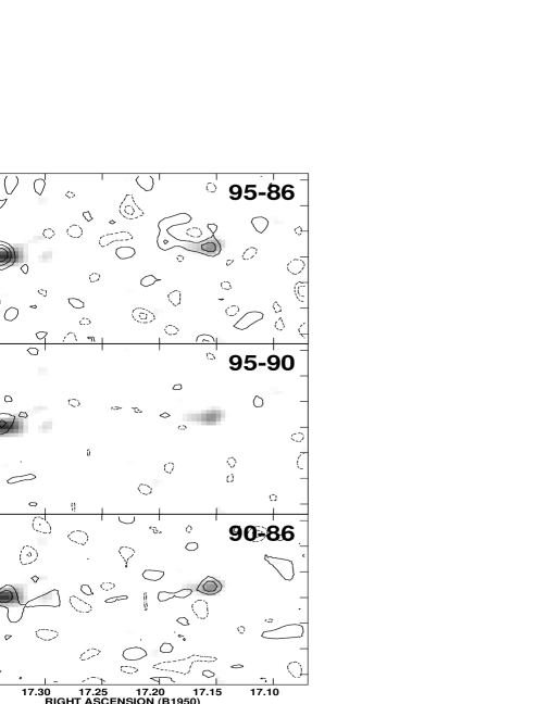
Figure 7: Difference map of the region around the synchrotron source, about $6^{\prime\prime}$ E of W 3(OH). The difference maps are shown in contour, and the image of the region is shown in gray-scale. The object to the left is the synchroton source, and the source to the right is believed to be its associated jet. The contour levels are $100\,\mu\rm Jy\,beam^{-1}$.

There is another feature which was present in the first epoch map but disappeared in those from later observations. The source, shown in Figure 8, is located about $7^{\prime\prime}$ NE of the main source, and is nearly unresolved. We identify this source with the ‘new source’ described in Baudry et al. (1993), who measured a flux density of 0.8 mJy and a peak brightness temperature of 750 K at 8.1 GHz. There is a nearby weak 1.6 GHz OH maser, which is probably excited by the source. In 1986 the source had a 15 GHz flux density of $1.0\,\rm mJy$, and then the source went below the detection threshold in 1990 and 1995. At the later epochs, we can place an upper limit of $0.1\,\rm mJy$ to the flux density.

Figure 8: A source $7^{\prime\prime}$ NE of the main source first described by Baudry et al (1993). The top panel is a map from the 1986 observations; middle, 1990; and bottom, 1995. The contour levels are $100\,\mu\rm Jy\,beam^{-1}$.

Baudry et al. (1993) observed this source in March, 1990, nearly at the same time as the 1990 epoch observations. If we assume that we have properly identified the source, there are three possibilities of what happened. The first one, which we feel is most likely, is that the source had already “turned off” before March 1990, and has a negative spectral index, making this object perhaps similar to the $\rm H_{2}O$ maser source immediately to its south. The other possibility is that the source “turned off” between Baudry’s March 1990 and our March 1990 observations, which would mean that we cannot infer any information about its spectral index. This possibility is not unphysical, since there is sufficient time between the observations for such a change to occur. Finally, it is also possible that this source is cosmological, and completely unrelated to the molecular cloud complex. However, Baudry et al. (1993) calculated that the the number of detectable extragalactic sources of greater or same brightness as the source, and concluded that such sources would be exceedingly rare. Also, the vicinity of the OH maser and the source suggests there is a relation between the two.

4 Discussion

4.1 A static model for W 3(OH)

In order to understand better the physical conditions in and around the H ii region, we have constructed a static model for the H ii region. Dreher & Welch (1981) attempted to model the H ii region as a spherical shell of ionized gas, but realized that this model could not reproduce the high degree of limb brightening that is actually observed. Moreover, rather than having a single model to describe the H ii region, the authors used different parameters to fit the brightness profiles along cuts made along the major and minor axes. The model is a spherical shell with inner and outer radii of 1300 AU and 1900 AU, respectively, with an electron density of $\sim 2\times 10^{5}\,\rm cm^{-3}$. They inferred an electron temperature of $9400\pm 1500\,\rm K$ by comparing the peak brightness in their 2 cm and 1.3 cm maps. Although the spherical models give a reasonable representation of the nebulae, the prolate ellipsoidal model, combined with the new observations, gives a better accounting for its structure and a better estimate of the density of the material in the shell.

From the present 2 cm and 1.3 cm maps, we can similarly measure the electron temperature. The peak brightness temperature occurs near the northern limb and is $10700\pm 500\,\rm K$ at 15 GHz and $8900\pm 500\,\rm K$ at 22 GHz. With these numbers we infer an electron temperature of $11000\pm 1600\,\rm K$, which is somewhat higher than but within error of that measured by Dreher & Welch (1981). However, there appears to be some non-uniformity of the temperature within the nebula, ranging from $\sim 9300\,\rm K$ near the western limb and $\sim 10^{4}\,\rm K$ near the southern limb. For the modeling described below, we adopt an average electron temperature of $10^{4}\pm 1000\,\rm K$.

The prolate ellipsoidal model has been successful in accounting the appearance of a number of planetary nebulae with widely varying morphology, despite its simplicity (Masson 1986). The model assumes a shell of uniform density, whose thickness varies as the inverse square of the distance from the central star. This property approximately accounts for the inverse square dilution of the radiation field. In essence, it ensures that the number of ionized gas particles in any solid angle viewed from the star is the same regardless of the direction. In a spherical model high limb-brightening can only be obtained by invoking a very thin shell. In our prolate model with ionization constraints, the ends of the shells are necessarily fainter than the equator, so lines of sight which pass closer to the major axis show greater degrees of limb brightening. The model has 6 parameters: opacity, minor and major axes of the ellipsoid, thickness of the shell at the minor (or major) axis and the angle of the tilt with which the H ii region is seen. The model is constrained by flux measurements of the source, temperature measurements of the gas, and the size and shape of the emission.

The contour maps of the model and the actual H ii region are shown in Figure 2. For presentation the contour map of W 3(OH) has been rotated by $30^{\circ}$ in position angle. The brightness along cuts made through the apparent major and minor axes are shown along the graph axes. In the model the electron temperature is assumed to be $10^{4}\,\rm K$ and the density $n_{e}=1.1\times 10^{6}\,\rm cm^{-3}$. The shell minor axis radius is $0.\kern-3.00003pt^{\prime\prime}\kern-1.00006pt5$, the major axis radius, $0.\kern-3.00003pt^{\prime\prime}\kern-1.00006pt95$, and the thickness on this minor axis is $0.\kern-3.00003pt^{\prime\prime}\kern-1.00006pt13$. The angle between the plane of the sky and the major axis is $10^{\circ}$. The total mass in the ionized shell is $0.013\,M_{\odot}$.

The thickness of $0.\kern-3.00003pt^{\prime\prime}\kern-1.00006pt13$ along the minor axis means that on the major axis, the thickness is less than $0.\kern-3.00003pt^{\prime\prime}\kern-1.00006pt04$, or about 80 AU. This is a consequence of the assumption of constant density in the ionized gas, and the ionization constraint could alternatively be satisfied by a thicker shell of lower density gas. However, a careful inspection of the brightness profile along the major axis in Figure 2 shows that there are small peaks at the edges of the emission region. This feature is reproduced in the model, and is a consequence of having a very thin shell. Another possible origin of the peaks is insufficient deconvolution of the maps. However, if this were the case, there would be negative features of roughly the same magnitude around the source, which are not present in the maps. It is likely that the actual shell is incomplete with gaps in some areas, especially near the poles of the prolate shell. Towards the eastern limb there is evidence of an “champagne-type” flow emerging, leading to a large area of low-emission level to the NE of the main source (Baudry et al. 1993; Keto et al. 1995), which is discussed in §4.4.

The simple model described here cannot reproduce the bright notch on the northern limb, nor the tail of emission that extends towards the east. As Dreher & Welch (1981) noted, the H ii region is also clumpy, which becomes more evident in their 1.3 cm maps. The present model does not consider the lateral spreading of ionizing photons within the shell, but effects caused by this should be mostly washed out on the size scale of the beam. Finally, a careful inspection of W 3(OH) reveals many fine, wispy structures. No simple model can sufficiently accommodate all such features.

4.2 Molecular environment surrounding the H ii region

By combining the measurement of the angular expansion rate and the density in the ionized shell determined from the model, we can estimate the physical conditions in the region immediately bordering the ionization front and in the ambient region ahead of the shock. These estimates of the physical conditions may then be compared with observed values. For the purpose of simplicity, the ionized shell will be assumed to have spherical symmetry, and we use parameters appropriate to the equatorial region of the shell. This is adequate because the aspect ratio of the model is $0.5:0.95$, which is less than the typical fractional uncertainty of observational measurements and is certainly less than the fractional uncertainties we expect from the estimates in the following discussion. Furthermore, since the real conditions are complicated by clumping and gradient effects, the estimates computed below should be taken to indicate average conditions near the H ii region.

We draw on an analysis which has been carried out by many workers (cf. Spitzer 1978). In this picture the H ii region is excited by a central star with a constant output of ionizing photons. The H ii region is a thin shell, which is radially expanding with a velocity $v_{i}$ with a uniform number density $n_{i}$. The H ii region is bordered by a discontinuous ionization front, where the hot ionized gas meets the shell of molecular material. This neutral shell is relatively thin, but since its bulk velocity is supersonic, there is a shock where the shell impacts the ambient material.

The total amount of material in the shell enclosed in a region less than a distance $r$ from the star is constant: $r^{3}n=\rm constant$. This implies that at the ionization front $3v_{i}n=-r_{i}\dot{n}_{e}$, where the subscript $i$ indicates parameters for material that is immediately next to the ionization front. In order to relate $v_{i}$ to the ionization front velocity, $V_{i}$, we recall that the total number of recombinations in the shell is also constant: $r_{i}^{3}n^{2}=\rm constant$, where $r_{i}$ is the radius of the ionized region. This equation implies that $3V_{i}n_{e}=-2r_{i}\dot{n}_{e}$ at the ionization front. Hence, the velocity of the ionized material can be related to the movement of the ionization front: $v_{i}={1\over 2}V_{i}$. The velocity of ionized gas with respect the ionization front at rest is $u_{i}={1\over 2}V_{i}$.

It is then a simple matter to calculate the conditions across the ionization front. First, we assume that the sound speed in the neutral region is negligible. The value of $u_{i}$ indicates that the ionization front is density-critical, and that the ram pressure of the ionized material is insignificant compared to its thermal pressure. Thus, the ratio of the density in the neutral shell to that in the ionized region may be expressed as $\rho_{s}/\rho_{i}=c_{s}^{2}/c_{i}^{2}$, where $c_{s}$ and $c_{i}$ are the sound speed in the neutral shell and ionized region, respectively. This expression may be then expressed as $n_{s}T_{s}=n_{i}T_{i}$, where $n_{s}$ and $n_{i}$ are the number density in the ionized and neutral regions. Here we assume an isothermal gas, and ignore the pressure arising from the magnetic field and turbulence.

The temperature of the ionized gas is taken to be $T_{i}=T_{e}=10^{4}\,\rm K$, which is typical of temperatures in H ii regions. The density of the H ii region, taken from the model in §4.1, is $n_{i}=1.1\times 10^{6}\,\rm cm^{-3}$, where we assumed that $n_{i}=n_{e}$. The physical conditions in the shocked shell may be inferred from observations of hydroxyl masers, which are believed to be harbored in the same dense shell of material adjacent to the H ii region (Moran et al. 1968, Reid et al. 1980). The masers occur in warm, dense clumps of molecular material, with $T\sim 150\,\rm K$, $n\sim 10^{6-8}\,\rm cm^{-3}$ (Reid & Moran 1988). From VLBI proper motion observations of these masers, Bloemhof et al. (1992) determined that they are also undergoing expansion at a speed of $\sim 3\,\rm km\,s^{-1}$, a value which is consistent with the observed expansion velocity of the ionization front, lending support to the claim that these masers occur in the expanding neutral shell. However, these masers occur in discrete clumps, with sizes $d\sim 10^{14}\,\rm cm$ across, and hence the density range given above are only characteristic of the conditions inside a masing region, which is a very small fraction of the volume. Observations of highly excited transitions of OH, which probably only arise in the warm and dense environment that also fosters the OH masers, indicate that the average density is $n\sim 7\times 10^{6}\,\rm cm^{-3}$ and $T\sim 150\,\rm K$ (Cesaroni & Walmsley 1991, Baudry et al. 1981). Taking $n_{s}=1\times 10^{7}\,\rm cm^{-3}$, we find that the pressures are somewhat different, $n_{s}T_{s}=1\times 10^{9}\,\rm K\,cm^{-3}$ and $n_{i}T_{i}=1\times 10^{10}\,\rm K\,cm^{-3}$. The latter quantity suggests that the number density in the shocked shell should be about $n_{s}=7\times 10^{7}\,\rm cm^{-3}$, which is the upper limit to the density estimate given by Reid & Moran (1988). Such a high density, however, is more favorable to the formation of high-gain masers. We may be able to reconcile this slight discrepancy, however, with the presence of a magnetic field.

If the magnetic field is sufficiently strong, then it can play an important role in the dynamics of the H ii region and its immediate neighborhood. The effect of magnetic fields is particularly important in strong shocks, because their presence limits the degree to which shocked gas can be compressed. Also, if the Alfvén speed exceeds the sound speed, then the magnetic field can dominate the energy transfer through a medium. However, the measurements of magnetic field strengths are difficult, and within the ionized region, such measurements do not exist. Also, it is necessary to have some information about the direction of the magnetic field with respect to the ionization front, but this is not readily observed. Therefore the conditions near the shock fronts cannot be modeled precisely.

The measurements of the magnetic field near W 3(OH) have been made by observing the Zeeman effect in hydroxyl masers. At the positions of the OH masers the typical magnetic field strength is $B_{tot}\sim 5\,\rm mG$ (Moran et al. 1968, Reid et al. 1980). Recently, Güsten, Fiebig & Uchida (1994) measured $3.1\pm 0.4\,\rm mG$ from observations of thermally excited OH. With this field strength, the magnetic field pressure in the gas is $B^{2}/8\pi\sim 6\times 10^{-7}\,\rm dyne\,cm^{-2}$, which is higher than the thermal pressure in the neutral gas by an order of magnitude, $nkT\sim 2\times 10^{-8}\,\rm dyne\,cm^{-2}$. Furthermore, as noted by Reid, Myers & Bieging (1987), the thermal pressure in the ionized material of the H ii region is nearly equal to the magnetic pressure in the neutral region, suggesting that the magnetic field must play an important role in the dynamics of the UCH ii region. However, they do not elaborate this assertion. Reid et al. (1987, Table 1) also tabulate the thermal, magnetic, turbulent and ram pressure contributions in the H ii region and molecular envelope.

To approximate the effect of the magnetic field at ionization front, the ratio of densities can be approximated to first order by $n_{s}/n_{i}=v_{A}^{2}/c_{i}^{2}$, where we replace the sound speed by $v_{A}$, the Alfvén speed. With this approximation, we see that $n_{s}/n_{i}\sim 4$, which is more consistent with the observed data, but surely a very crude estimate. At the shock front the magnetic field pressure dominates the thermal pressure but is comparable to the ram pressure. Thus the effect of the magnetic field is to push the ratio of the densities in the shell region and the ambient medium closer to unity. Thus, although the observations do not permit us a detailed analysis of the ionization front, it is clear that magnetic fields play an important part.

Ahead of this shell of neutral material, there is a shock as the shell impacts the ambient material. Making a similar analysis, we find that at the shock front, $P_{i}=\rho_{a}V_{s}^{2}$, where $\rho_{a}$ is the density of the ambient gas. In this case most of the pressure is supplied by the ram pressure, because the temperatures of the gases are not very different, and the sound speed is much smaller than the expansion rate. This expression predicts that the ambient number density to be $n_{a}/n_{s}=c_{s}^{2}/V_{s}^{2}=0.1$. The ambient material can be probed by observing molecular lines in absorption against the H ii region, although with this method some of the gas in the shocked region will be sampled as well. Absorption of $\rm H_{2}CO$ near the velocity of the OH masers indicates that the density of the foreground $\rm H_{2}$ number density ranges from $n<10^{3}\,\rm cm^{-3}$ towards the eastern limb to $n>5\times 10^{5}\,\rm cm^{-3}$ in the west (Dickel & Goss, 1987). This is consistent with the density observed in the regions harboring OH masers.

In our simple analysis, we have ignored the effects of turbulence, which has been proposed as a mechanism through which UCH ii regions attain their longevity (Xie et al. 1996). The effects of turbulence is usually treated simply as an extra pressure term, $P_{turb}$. The pressure arising from turbulence is particularly important in the H ii region, where its value is comparable to the thermal pressure. This would mean that more pressure is needed from the shocked gas, but would change the value of the density by less than an order of magnitude.

4.3 Stellar wind and radiation pressure

Soon after the central star in W 3(OH) reached the main-sequence, the stellar wind and radiation pressure drove away the circumstellar material to evacuate a cavity, and the H ii region was formed from the inner edge of the shell of material (Davidson & Harwit 1967). Presumably, this is picture still applies to W 3(OH).

In order to maintain the shell structure, and to keep it expanding, there has to be some pressure being exerted from inside the shell. The magnitude of the pressure necessary to support the shell can be easily estimated by setting the thermal pressure in the ionized region equal to the ram pressure in the rarefied region, $P_{ram}=2n_{e}k_{B}T_{e}$. The two possible forces responsible for this pressure are the stellar wind composed of material from the star and radiation pressure acting upon dust in the shell.

It is well-known that early-type stars possess fast strong stellar winds, $v_{w}\sim 1000\,\rm km\,s^{-1}$ and associated mass loss, $\dot{M}\sim 10^{-6}\,M_{\odot}\,\rm yr^{-1}$ for an O7 star, although the nature of their mechanism is poorly understood (e.g. Chiosi & Maeder 1986). If we assume that the mass loss is isotropic, then the ram pressure of the stellar wind is $P_{w}=\dot{M}v_{w}/4\pi r^{2}$, where $r$ is the distance of the shell from the star. The wind pressure is $P_{w}=2\times 10^{-6}\,\rm dyne\,cm^{-2}$, which is nearly equal to the thermal pressure of the gas, $P_{i}=3\times 10^{-6}\,\rm dyne\,cm^{-2}$. Thus we calculate there is sufficient ram pressure from the stellar wind to sustain the shell structure in W 3(OH).

The radiation from the central star is first absorbed by dust particles, which share their momentum with the gas through collisions. Dreher & Welch (1981) show that about two-thirds of the ultra-violet radiation is absorbed by dust in the ionized shell. The pressure from the dust can similarly be expressed as, $P_{rad}=\beta L/4\pi r^{2}c$, where $L$ is the luminosity of the star, $c$ is the speed of light, and $\beta$ indicates the fraction of the radiation that is absorbed by the dust, which in this case is about unity. We calculate that $P_{rad}=3\times 10^{-6}\rm\,dyne\,cm^{-2}$, which is almost equal to the stellar wind pressure.

The outward pressures stated above represent merely lower limits to the actual values. Nevertheless, it is quite clear that there is sufficient pressure from either these mechanism to evacuate W 3(OH) and to keep it expanding. It is not possible to determine which process dominates in evacuating the shell, although they probably work in parallel.

4.4 A dynamical model for W 3(OH)

One of the most perplexing aspects of W 3(OH) is the systematic blue-shifting and broadening of hydrogen recombination lines with increasing quantum number. Early observations of the region with centimeter-wave interferometers revealed that there was a significant velocity difference between the foreground molecular material, probed by OH masers (Reid et al 1980) or methanol absorption lines (Reid et al 1987), and that of the ionized region, probed by high-quantum number recombination lines of hydrogen (Hughes & Viner 1976). Reid et al (1987) measured a difference of about $5\,\rm km\,s^{-1}$, which they interpreted as infall of the molecular material towards the star. However, observations of recombination lines at higher frequencies (lower quantum numbers) showed that the velocity difference becomes less. In a prescient paper, Berulis & Ershov (1983) attributed this trend to non-LTE effects in a rapidly expanding ionized shell. The shell was thought to be expanding at $18\,\rm km\,s^{-1}$. Further study was permitted by the advent of millimeter-wave interferometers, and Welch & Marr (1987) showed that the velocities of the recombination lines at lower quantum numbers closely approach those of molecular lines. They concluded that the infall model was wrong, and also the line width of the recombination line was too narrow for the source to be rapidly expanding.

The present observations unambiguously preclude the rapidly expanding shell model of Berulis & Ershov (1983), unless the expansion only occurs along the viewing axis, which seems highly unlikely. More recent attempts to describe W 3(OH) are the cometary stellar-wind bow shock (Van Buren et al. 1990), the line-broadened fast flow (Keto et al. 1995), and the two layer cloud model (Wilson et al. 1991).

Our expansion measurements do not support the suggestion by Bloemhof et al. (1992) that W 3(OH) is a cometary stellar-wind bow shock (Van Buren et al. 1990). The cometary bow shock model was specifically proposed to explain the longevity of UCH ii regions. In the bow shock model the central star has a large velocity relative to the surrounding molecular cloud, and the stellar wind pushes aside the oncoming molecular material. The ram pressure of the swept-up molecular material effectively confines the H ii region, and its age is thus considerably longer than indicated by the dynamical age. Furthermore, the cometary phase may last as long as there is sufficient material near the star: as it traverses different molecular cloud clumps, the cometary bow shock may reform a number of times. Most relevant to our observations, the bow shock structure can only appear to expand if the star is moving from a more dense to a less dense region of the molecular cloud. We make a simple estimate of the required density gradient as follows.

In the simple stellar-wind bow shock model an early type star is assumed to plow through a molecular cloud at a supersonic speed of about $6\,\rm km\,s^{-1}$. Since Welch & Marr (1987) determined that the relative velocity along the line of sight between the W 3(OH) H ii region and the molecular cloud is less than $1.3\,\rm km\,s^{-1}$, the hypothetical velocity of $6\,\rm km\,s^{-1}$ must occur in the plane of the sky, possibly to the SW (Bloemhof et al 1992). The radius, $l$, of the bow shock is determined by pressure balance between the stellar wind and the ram pressure, and is given by $l\sim n^{-1/2}$ (van Buren et al 1990). The apparent expansion of the H ii region owing to density variations in the molecular cloud may be written as $\epsilon=-d(\ln n_{a})/dr(v_{s}/2)$, where $1+\epsilon$ is the expansion factor, $n_{a}$ is the number density of the ambient medium. By simply solving for the gradient, we compute the lower limit to the density gradient: $d(\ln n_{a})/dr>140\,\rm pc^{-1}$. Given the size of W 3(OH), we estimate that density has to be falling off by a factor of at least 4 from NE to SW across the H ii region. This is in direct contradiction to what is generally observed using various molecular tracers, where the gradient goes in the opposite sense (e.g., Dickel & Goss 1987). Furthermore, if there were such a gradient to begin with it is very difficult to believe that W 3(OH) would be presently so symmetrical, since the radius should change by a factor of 2 across the region.

Keto et al. (1995) modeled the W 3(OH) as a fast flow of ionized gas moving towards the observer that included the effects of pressure broadening in the gas. The flow is densest at its origin, nearest the star, and becomes less dense further along the flow. The flow fills a paraboloid, and the velocity of the material is fixed to conserve mass. For a viewer looking down the flow, the recombination line from the gas to the foreground is optically thin, blue-shifted, and has a thermal line width. However, at the densest part of the flow, the same recombination line is pressure-broadened and is effectively made optically thin. (The opacity integrated over a large velocity range, however, is still proportional to $n_{e}^{2}$.) The effects of pressure broadening, however, decreases at lower quantum numbers. Therefore, the millimeter-wavelength recombination lines will appear thermally broadened and centered at about the same frequency as the molecular gas. At lower frequencies the line becomes broader and more blue-shifted. Keto et al. (1995) also try to account for the observed shell structure using the flow. Specifically, they tilt the parabolic flow so that the flow resembles the shape of W 3(OH), with the opening pointing towards the northeast. The tilted parabolic flow qualitatively describes both the observed structure and the velocity gradient in the recombination line across the major axis of the H ii region. Finally, to account for the limb brightening, the inner one-sixth of the parabola is left without any material flowing through it.

Although the model gives good agreement to the line width and line velocity data, the only physical constraint in the model is mass conservation. Furthermore, Keto et al. (1995) do not propose any physical mechanism responsible for the flow other than to invoke the well-known champagne flow model of Tenorio-Tagle (1979). There are several salient problems even in the simple model they present. First, when the emission measure is calculated from the parameters they give for the flow, it falls short of the observed value. An upper limit to the emission measure may be calculated as $EM=n_{0}^{2}z_{0}/(2\alpha_{ne}-1)\approx 2\times 10^{7}\,\rm cm^{-6}\,pc$, where we use the numbers provided by Keto et al. (1995) and use their notation. Here, $n_{0}$ is the maximum density, $z_{0}$ describes the size scale of the H ii region, and $\alpha_{ne}$ is the exponent by which the density in the region falls off in units of $z_{0}$. We assume that $z_{0}$, which is not mentioned in their paper, is the size of the H ii region itself. The actual EM is about 50 times higher. Thus the flow they describe is optically thin.

Since the flow is optically thin, we might consider a model in which this parabolic flow is actually emerging from the optically thick shell shell. This description is somewhat similar to that given by Wilson et al. (1991) who modeled the H ii region as being composed of two discrete layers of ionized gas moving at different velocities. In this configuration the observed recombination lines would mainly trace the rarefied fast flow because those that originate in the shell are severely pressure-broadened. As noted in §4.1, there is extended emission towards the NE edge of W 3(OH), and we can picture that the fast flow is emerging from the optically thick shell to the foreground.

In this configuration the apparent expansion velocity of shell would be slightly higher than that of the actual bulk motion of the ionized gas, since the radiation can reach further into the neutral medium as the region gets evacuated. We establish that in order to maintain such a flow for an extended period of time, the ionized material must continually be replenished. The time scale for the flow to evacuate the ionized region without replenishment is given by $t_{evac}=M/\dot{M}\sim 1000\,\rm yr$, where $M$ is the mass of the ionized region, and $\dot{M}=vnAm_{H}$ is the mass flux. In the expression for the mass flux $v$ is the velocity of the flow, $n$ is the number density of the flow, $A$ is the cross-sectional area, and $m_{H}$ is the proton mass. Here, we assumed that the scaling length $z_{0}$ in Keto et al. (1995) is the about the same size as the H ii region, $\sim 2\times 10^{16}\,\rm cm$. If the material is replenished from ionization front, then there should be an apparent movement of the ionization front. We can estimate this movement as $v\sim\dot{M}/4\pi r^{2}n$, where $r$ is the radius of the shell. We estimate that $v\sim 2\,\rm km\,s^{-1}$. If the depletion of gas is contributing to the movement of the ionization front, then the masers would appear to expand at a slightly slower speed than the ionization because the bulk movement of the gas would still be determined by radiation or stellar wind pressure. The ionized region does seem to be expanding slightly faster than the masers, although the uncertainties are rather too high to make a decisive conclusion.

We should note that the fast flow model does not adequately agree with several important observational facts. Keto et al. (1995) observed that the $\rm H92\alpha$ line velocity has a gradient of $18\,\rm km\,s^{-1}$ from E to W. When the velocity gradient across the source is calculated from the model, it cannot easily reproduce the observed gradual shift in the recombination line velocity across the source. Furthermore, it may be merely a coincidence that the major axis of W 3(OH) is in the same direction as the velocity gradient. For example, in the case of G34.3, another bright, well-studied UCH ii region, the gradient in the velocity of the recombination line is transverse to the long axis of the UCH ii region (Gaume et al. 1994). The model also makes definite predictions about the lineshapes. The line profiles of millimeter-wave recombination lines have a blue-shifted shoulder because while the bulk of the emission originates at the densest area, the higher velocity material still makes a contribution. Unfortunately, the line profile of $\rm H35\alpha$ does not show even a hint of asymmetry (Wilson et al. 1987). The centimeter-wave line profiles should also be slightly asymmetric, with the shoulder on the low velocity side.

These discrepancies might lead us to conclude that rather than there being a fast flow, there might be layers of ionized gas moving more or less at discrete but uniform speed in the foreground of the main H ii region (Wilson et al. 1991). Wilson et al. (1991) modeled the H ii region as comprised of two components along the line of sight. The first clump has a higher density but smaller mass than the second clump, and the observer sees a blend of the two regions. With this configuration, Wilson et al. (1991) were able to reproduce the line width and line velocity data, and it seems that this model would readily reproduce the observed profiles of the recombination lines.

Thus, we come to the general conclusion that that the most satisfactory model for W 3(OH) is that it is comprised of two components, an optically thick shell and a related or separate regions of ionized gas in the foreground that are moving at different velocities. Ultimately, further constraints to models will have to come from better measurements of the recombination line profiles. The measurement of Wilson et al. (1987) favors the discrete cloud model.

4.5 Lifetime of the UCH ii phase

The direct measurement of the expansion rate in W 3(OH) gives us a good estimate of the age of the H ii region that is independent of any models: The age of the shell is only $2.3\times 10^{3}\,\rm yr$. This assumes that the expansion velocity has been constant in time, which, of course, is a simplified picture. If we linearly extrapolate to the future, then W 3(OH) would cease to become an ultra-compact H ii region in about $2\times 10^{4}\,\rm yr$. This is within an order of magnitude of the expected duration of the ultra-compact phase.

In another simple analysis we can apply the classical equation that governs the expansion rate of an H ii region once it has reached the Strömgren radius. This was first applied to the study of UCH ii regions by De Pree, Rodríguez & Goss (1995), who proposed that if the molecular gas in which the H ii region initially formed is sufficiently dense and warm, the ambient pressure may be sufficient to confine the H ii region for at least $10^{5}\,\rm yr$. We take their example of an O6 star which formed in an ambient density of $n=2\times 10^{7}\,\rm cm^{-3}$. These conditions are reasonable since they are close to the values used for the static model for the shell. The initial Strögrem sphere is only $10^{-3}\,\rm pc$ in radius, and the initial rate of expansion is at the plasma sound speed. To expand to a diameter of 0.01 pc, which is the present size of W 3(OH), it takes only 900 yr, but by this time, the rate of expansion has slowed to $4\,\rm km\,s^{-1}$. This value for the expansion rate is in remarkable agreement with our measured value. In this analysis the expansion rate continues to decrease with time, and at the end of $10^{5}\,\rm yr$ the H ii region reaches a diameter of only $0.14\,\rm pc$. Therefore, in the context of this picture although the H ii region is relatively young, W 3(OH) can apparently remain in the UCH ii phase for almost $10^{5}\,\rm yr$.

In summary it appears that the major properties of the W 3(OH) H ii region can be satisfactorily explained by invoking simple, classical ideas regarding the Strögrem sphere. Though the H ii region is probably be very young, the predicted time it will remain in the UCH ii phase is comparably long to what is expected. The complete picture, is obviously more comlicated than this. For example, since the density gradient would favor faster expansion rates as the region gets larger, the extrapolated lifetimes from the simple analyses might be considered an upper limit. The uncertainties regarding the molecular environment and stellar wind, radiation, and magnetic pressure make it difficult to predict very accurately the expected life time of the ultra-compact phase.

Finally, it is important to distinguish the age of the structure of an H ii region from the actual duration of the ultra-compact phase: the two are not necessarily related. The appearance of the ionized gas may change quite rapidly. Thus, the dynamical age may not indicate the actual age of the H ii region at all. Indeed, in W 3(OH), the shell structure may well disappear in a rather short period of time, if the shell breaks out of the core of the molecular cloud; it would then take on a different appearance, perhaps a core-halo structure. Hence, it will still be an UCH ii region. Since there is evidence of activity near the central star (§4.6) this is a tantalizing possibility, although it is merely a speculation.

4.6 Emission near the central star

As we noted earlier, there is a feature very close to the projected center of the H ii region that exhibits rapid variability, and owing to its location we tentatively link to the central star. If the change in flux at this source can be entirely attributed to mass loss from the region, we infer that the density in the region fell by $\sim 2\times 10^{5}\,\rm cm^{-3}$. If this mass left the region enclosed by $\sim 300\,\rm AU$ around the star within a period of $<4\,\rm yr$, this represents a mass loss of $\sim 10^{-6}M_{\odot}\,\rm yr^{-1}$, which is a value remarkably close to the wind mass loss rate of the star.

Curiously, this value for the mass loss is of the same order of the mass flux expected from the photoevaporation disk model (Hollenbach et al. 1994), and the size scale is also roughly the size of most disk models as well. Furthermore, another approximation can be made: because there are positive features beside the negative feature, a crude velocity may be estimated if we interpret these features to be movement of gas material. The positive features are roughly $0.\kern-3.00003pt^{\prime\prime}\kern-1.00006pt1$ from the negative peak. If this represents a movement of gas, it would correspond to a velocity of $\sim 300\,\rm km\,s^{-1}$. This is the characteristic speed of a stellar jet.

5 Conclusion

We have made direct measurements showing that the UCH ii region W 3(OH) is expanding at $\rm 3\,\,to\,\,5\,km\,s^{-1}$. The expansion rate also implies directly that the age is $\sim 2300\,\rm yr$, much lower than the $10^{5}\,\rm yr$ believed to be typical for UCH ii regions. The new data are consistent with a simple physical model in which the OH masers are in a dense, shocked neutral shell swept up around the UCH ii region, which is expanding anisotropically into the surrounding molecular cloud. Within this simple model there is apparently no difficulty with the age issue regarding UCH ii regions. In addition, from the difference maps we have detected a number of interesting sources, most notably the variability linked to the central star. There is a clear need to study this particular source and other flickering objects in greater detail.

The technique of generating difference maps could be applied to a few of the brightest shell or cometary UCH ii regions. It was recently applied to observe an apparent expansion in G5.89$-$0.4, a well-studied bright shell-shaped UCH ii region (Acord, Churchwell & Wood 1998). Acord et al (1998) concluded that the H ii region is expanding at $35\,\rm km\,s^{-1}$. It should be stressed that the expansion signature can be best translated into a velocity when there are sharp features in the maps, like those found in an ionization-bounded nebula. G5.89 has an extended region of emission around the limb-brightened shell, and this makes the proper motion measurements somewhat ambiguous. However, an important result from Acord et al (1998) is that the time-scale for gross change in the emission structure of the H ii region is of order less than 100 yr. We conclude that W 3(OH) is quite distinct from G5.89, despite their similar morphology. Regardless, this short time-scale clearly has important implications for the study of UCH ii in general. We have already tried the same experiment on a core-halo region, NGC 7538 (Kawamura 1997). Although large differences were observed between maps at different epochs, there was no clear pattern and it was hard to make a simple physical model.

We thank the anonymous referee for suggesting that we expand our discussions regarding the cometary bow-shock model and the lifetime issue.

References

- (1)
- (2) Acord, J. M., Churchwell, E., & Wood, D. 1998 ApJ, 495, L107
- (3)
- (4) Akeson, R. L. & Carlstrom, J. E. 1996 ApJ, 470, 582
- (5)
- (6) Baudry, A., Menton, K. M., Walmsley, C. M., & Wilson, T. L. 1993, A&A, 271, 552
- (7)
- (8) Berulis, I. I. & Ershov, A. A. 1983, Soviet Astron. Lett., 9, 6
- (9)
- (10) Bloemhof, E. E., Reid, M. J., & Moran, J. M. 1992 ApJ, 397, 500
- (11)
- (12) Cesaroni, R. & Walmsley, C. M. 1991, A&A, 241, 537
- (13)
- (14) Chiosi, C. & Maeder, A. 1986, ARA&A, 24, 329
- (15)
- (16) Davidson, K. & Harwit, M. 1967, ApJ, 148, 443
- (17)
- (18) De Pree, C. G., Rodríguez, L. F., & Goss, W. M. 1995, Revista Mexicana de Astronomía y Astrofísica, 31, 39
- (19)
- (20) Dickel, H. R. & Goss W. M. 1987 A&A, 185, 271
- (21)
- (22) Dreher, J. W. & Welch, W. J. 1981, ApJ, 245, 857
- (23)
- (24) García-Segura, G., & Franco, J. 1996, ApJ, 469, 171
- (25)
- (26) Gaume, R. A., Fey, A. L., & Claussen, M. J. 1994, ApJ, 432, 648
- (27)
- (28) Güsten, R., Fiebig, D., & Uchida, K. I. 1994, A&A, 286, L51
- (29)
- (30) Habing, H. J., & Israel, F. P. 1979, ARA&A, 17, 345
- (31)
- (32) Hollenbach, D., Johnstone, D., Lizano, S., & Shu, F. 1994, ApJ, 428, 654
- (33)
- (34) Hughes, V. A. & Viner, M. R. 1976, ApJ, 204, 55
- (35)
- (36) Humphreys, R. M. 1978, ApJS, 38, 309
- (37)
- (38) Kawamura, J., 1997, Ph.D. Thesis, Harvard University.
- (39)
- (40) Keto, E. R., Welch, W. J., Reid, M. J., & Ho, P. T. P. 1995, ApJ, 444, 765
- (41)
- (42) Larson, R. B. 1969a, MNRAS, 145, 271
- (43)
- (44) Larson, R. B. 1969b, MNRAS, 145, 297
- (45)
- (46) Larson, R. B. 1972, A&A, 37, 149
- (47)
- (48) Mac Low, M.-M., Van Buren, D., Wood, D., & Churchwell, E. 1990, ApJ, 369, 395
- (49)
- (50) Masson, C. R. 1986, ApJ, 302, L27
- (51)
- (52) Moran, J. M., Burke, B. F., Barrett, A. H., Rogers, A. E. E., Carter, J. C., Ball, J. A., & Cudaback, D. D. 1968, ApJ, 152, L97
- (53)
- (54) Norris, R. P. & Booth, R. S. 1981, MNRAS, 195, 213
- (55)
- (56) Reid, M. J., Argon, A. L., Masson, C. R., Menten, K. M., & Moran, J. M. 1995, ApJ, 443, 238
- (57)
- (58) Reid, M. J., Haschick, A. D., Burke, B. F., Moran, J. M., Johnston, K. J., & Swenson, G. W. 1980, ApJ, 239, 89
- (59)
- (60) Reid, M. J. & Moran, J. M. 1988, in Galactic and Extragalactic Radio Astronomy, ed. G. L. Verschuur & K. I. Kellermann (2d ed.; New York: Springer), 255
- (61)
- (62) Reid, M. J., Myers, P. C., & Bieging, J. H. 1987, ApJ, 312, 830
- (63)
- (64) Spitzer, L. 1978, Physical Processes in the Interstellar Medium. (New York: Wiley)
- (65)
- (66) Tenorio-Tagle, G. 1979, A&A, 71, 59
- (67)
- (68) Turner, J. L. & Welch, W. J., 1984, ApJ, 287, L81
- (69)
- (70) Van Buren, D., Mac Low, M.-M., Wood, D., & Churchwell, E. 1990, ApJ, 353, 570
- (71)
- (72) Welch, W. J. & Marr, J. 1987, ApJ, 317, L21
- (73)
- (74) Wilner, D. J., Welch, W. J., & Forster, J. R., 1995, ApJ, 449, L73
- (75)
- (76) Wilson, T. L., Johnston, K. J., & Mauersberger, R. 1991, A&A, 251, 220
- (77)
- (78) Wilson, T. L., Mauersberger, R., Brand, J., & Gardner, F. F. 1987, A&A, 186, L5
- (79)
- (80) Wink, J. E., Duvert, G., Guilloteau, S., Güsten, R., Walmsley, C. M., & Wilson, T. L., 1994, A&A, 281, 505
- (81)
- (82) Wood, D. O. S., & Churchwell, E. 1989a, ApJS, 69, 831
- (83)
- (84) Wood, D. O. S., & Churchwell, E. 1989b, ApJ, 340, 265
- (85)
- (86) Wynn-Williams, C. G., Becklin, E. E., & Neugebauer, G. 1972, MNRAS, 160, 1
- (87)
- (88) Yorke, H. W. & Krügel, E. 1977 A&A, 54, 183
- (89)
- (90) Xie, T., Mundy, L. G., Vogel, S. N., & Hofner, P. 1996, ApJ, 473, L131
- (91)