Using SCUBA to place upper limits on arcsecond scale CMB anisotropies at 850$\,\mu$m

Abstract

The SCUBA instrument on the James Clerk Maxwell Telescope has already had an impact on cosmology by detecting relatively large numbers of dusty galaxies at high redshift. Apart from identifying well-detected sources, such data can also be mined for information about fainter sources and their correlations, as revealed through low level fluctuations in SCUBA maps. As a first step in this direction we analyse a small SCUBA data-set as if it were obtained from a Cosmic Microwave Background (CMB) differencing experiment. This enables us to place limits on CMB anisotropy at 850$\,\mu$m. Expressed as $Q_{\rm flat}$, the quadrupole expectation value for a flat power spectrum, the limit is 152$\,\mu$K at 95 per cent confidence, corresponding to $C_{0}^{1/2}{<}\,$355$\,\mu$K for a Gaussian autocorrelation function, with a coherence angle of about 20–25 arcsec; These results could easily be reinterpretted in terms of any other fluctuating sky signal. This is currently the best limit for these scales at high frequency, and comparable to limits at similar angular scales in the radio. Even with such a modest data-set, it is possible to put a constraint on the slope of the SCUBA counts at the faint end, since even randomly distributed sources would lead to fluctuations. Future analysis of sky correlations in more extensive data-sets ought to yield detections, and hence additional information on source counts and clustering.

1 Introduction

Since COBE discovered the existence of anisotropy in the Cosmic Microwave Background Radiation (CMB) at large angular scales, balloon and ground based experiments have detected anisotropy at a range of smaller scales (see e.g. Smoot & Scott 1998). All cosmological models predict that the very smallest scales should be free of primordial anisotropy, because photons in small-scale overdensities which entered the horizon early have been able to random walk out of the potential wells, and also because fluctuations on scales below the thickness of the last scattering surface are suppressed.

Nevertheless, secondary anisotropies can be generated through a wide variety of physical processes occurring at redshifts $<1000$. For an overview of some of these effects see Bond (1996). There is new motivation from the detection of the Far Infrared Background (FIB, Puget et al. 1996, Schlegel, Finkbeiner & Davis 1998, Fixsen et al. 1998, Hauser et al. 1998), as well as recent SCUBA results, that dusty galaxies at high redshifts could be of greater significance than previously assumed – possibly the dominant source of CMB anisotropy at arcsecond scales, and certainly the dominant source of sky fluctuations at $\sim 1\,$mm, at least out of the galactic plane. The smooth FIB is expected to break-up into sources, plus fluctuations due to unresolved sources, and correlations between sources on the sky. Weak Sunyaev–Zel’dovich increments, caused by hot gas in virialised structures, may also contribute to anisotropies in the sub-millimetre, and of course other physical effects could also be important. We attempt here to use SCUBA data to place limits on general fluctuations within the framework of CMB anisotropies, i.e. as intensity fluctuations on a $2.728\,$K blackbody spectrum; but everything can be reinterpretted in terms of fluctuations of some other spectral component.

Experiments probing similar angular scales have already placed upper limits of anisotropy at a variety of wavelengths, and a summary can be found in Table 1. The results are generally quoted in terms of the most sensitive GACF (which will be described in Section 4), although a few experiments simply give a limit to the variance of the temperature measurements. Limits set at radio wavelengths are markedly more sensitive than those in the millimetre region. However, the expected foreground signals at low frequency are expected to be entirely different to those which are likely to dominate fluctuations in the sub-millimetre sky (namely dusty galaxies and hot cluster gas). The most relevant previous measurement is the earlier JCMT limit of Church, Lasenby & Hills (1993), using the single bolometer which was the predecessor to SCUBA.

Table 1: Summary of previous small angular scale CMB limits.

$\lambda$	Angular Scale	${\Delta T}/T$	Instrument	Reference
800$\,\mu$m	17 arcsec	$\leq 146\times 10^{-5}$	JCMT	Church et al. (1993)
1250$\,\mu$m	30 arcsec	$\leq 14\times 10^{-5}$	SEST & IRAM	Andreani (1994)
	70 arcsec	$\leq 24\times 10^{-5}$
	140 arcsec	$\leq 19\times 10^{-5}$
1300$\,\mu$m	12 arcsec	$\leq 18\times 10^{-5}$	IRAM	Kreysa & Chini (1989)
2110$\,\mu$m	66 arcsec	$\leq 2.1\times 10^{-5}$	SuZIE	Church et al. (1997)
3400$\,\mu$m	10 arcsec	$\leq 9\times 10^{-5}$	IRAM	Radford (1993)
15,000$\,\mu$m	156 arcsec	$\leq 1.7\times 10^{-5}$	OVRO	Readhead et al. (1989)
19,700$\,\mu$m	20 arcsec	$\leq 2.3\times 10^{-5}$	Ryle	Jones (1997)
35,000$\,\mu$m	30 arcsec	$\leq 2.3\times 10^{-5}$	ATCA	Subrahmanyan et al. (1998)
	60 arcsec	$\leq 1.6\times 10^{-5}$
	120 arcsec	$\leq 2.5\times 10^{-5}$
35,000$\,\mu$m	6 arcsec	$12.8\times 10^{-5}$	VLA	Partridge et al. (1997)
	18 arcsec	$\leq 4.8\times 10^{-5}$
	60 arcsec	$\leq 2.0\times 10^{-5}$

2 SCUBA Observations

The observations were conducted with the Submillimeter Common-User Bolometer Array [Cunningham et al. 1994, Gear & Cunningham 1995, Lightfoot et al. 1995] on the James Clerk Maxwell Telescope. SCUBA contains a number of detectors and detector arrays cooled to 0.1 K that cover the atmospheric windows from 350$\,\mu$m to 2000$\,\mu$m.

The arrays have a hexagonal arrangement of pixels, with feeds about two beamwidths apart in the focal plane. The two array detectors provide an instantaneous field-of-view of 2.3 arcmin and can be used simultaneously. They consist of the 91 element Short-wave array, which we used with the 450$\,\mu$m filter, and the 37 element Long-wave array, which we used at 850$\,\mu$m. An illustration of the observing strategy is given in Fig. 1, and described in more detail below. Essentially it is a double difference experiment, with some additional complications.

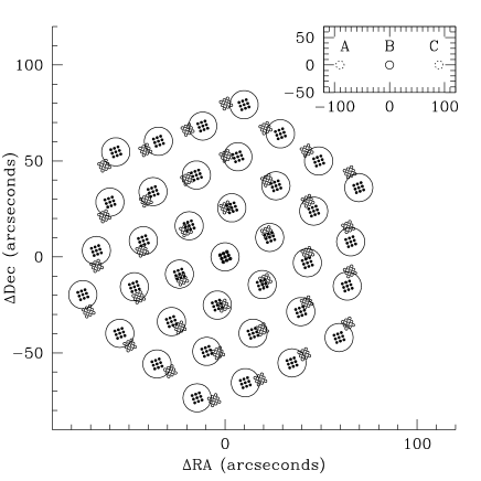
Figure 1: The arrangement of the 37 bolometers in the long wavelength array. The squares of 9 points are the jiggle positions that create an effective beam of 14.7 arcsec, which are shown as the larger circles on the main plot. The solid jiggle pattern shows the bolometer positions for the first integration. Due to earth rotation, the entire array rotates throughout the course of the run, and we have plotted the position of the bolometers for the last integration using open circles. The inset illustrates the three positions for the three beam chop that constitutes a single integration. The entire array is chopped in azimuth with this double-difference pattern.

During an integration, the telescope is ‘jiggled’ in a 3 $\times$ 3 square pattern (with 2 arcsec offsets, shown in Fig. 1). This improves the photometric accuracy, reducing the impact of pointing errors by averaging the source signal over an area slightly larger than the beam. The effective half-power beamwidths for the 450 and 850$\,\mu$m pixels are then 7.5 arcsec and 14.7 arcsec respectively.

Whilst jiggling, the secondary was chopped at 7.8125 Hz between two positions, $A$ and $B$, separated here by 90 arcsec in azimuth, yielding the single difference measurement $I_{B}-I_{A}$. This is followed by a second single difference, $I_{C}-I_{B}$, after the nod to the other side of $B$. By differencing these two differences, we obtain a series of double differences, with the signal defined by $S=-I_{A}+2I_{B}-I_{C}$. For some of the systematic checks we will consider the data on a jiggle by jiggle basis. However, the data are generally treated by lumping the 9 jiggles together, yielding an 18 second double difference for each bolometer, which we refer to as a single ‘integration’. Considered in this way the set-up is the traditional triple beam arrangement common in CMB experiments.

SCUBA can also use a 64 point jiggle in order to fill in the blank space between the pixels (‘mapping mode’), but for this initial study, we use ‘photometry’ observations at 450 and 850$\,\mu$m. Although this provides an undersampled map at both wavelengths, it is more straightforward to analyze.

On 1997 December 3, five ‘scans’ of 900 seconds, consisting of 50 integrations each were taken. The central pixel of SCUBA was fixed on a point source in an otherwise blank field, for which we were interested in obtaining sub-mm photometry (the lensed AGN B1933+503, Chapman, Fahlman & Scott, in preparation). The other pixels rotated relative to the sky through the period of the integration; we show the positions of the first and last integrations in Fig. 1. Pointing was checked hourly on the blazar 2036–419 and a sky-dip was performed between each 15 minute scan to measure the atmospheric opacity. The rms pointing errors were below 2 arcsec, while the average atmospheric zenith opacities at 450$\,\mu$m and 850$\,\mu$m were fairly stable with $\tau$ being 0.51 and 0.12 respectively. However, there were some short time-scale variations, presumably due to water vapour pockets blowing over at high altitude, which caused some parts of the data-set to be noisier (see Fig. 2. The observations were largely reduced using the Starlink package SURF (Scuba User Reduction Facility, Jenness & Lightfoot 1998). Spikes were first carefully rejected from the double difference data. The data were then corrected for atmospheric opacity and calibrated against Saturn and the compact H II region K3–50, which were also observed during the same observing shift. The 850$\,\mu$m calibrations agreed with each other and also the standard gains to within 10 per cent. However, at 450$\,\mu$m, K3–50 is extended and variable, and is not a good calibration source, while the Saturn 450$\,\mu$m calibration agreed with standard gains to within 25 per cent.

3 Data Reduction

It is necessary to identify and remove any non-astronomical signals from the data. One of SCUBA’s many strengths is its ability to redundantly measure the strongest of these contaminants: atmospheric emission. To a lesser extent, cosmic ray hits influence the data, but these are readily identified by the spikes they leave in the timestream, and are therefore easily removed from the data (more details in the next section). Finally, we test for other correlations in the data that indicate a common signal, such as cross-talk between bolometers.

In order to discuss our analysis procedure, we adopt the following notation. The indices $b,s,i,$ and $j$ denote bolometer, scan, integration, and jiggle number respectively, each starting at 1. The variable $N$ subscripted with one of these indices represents the total number of the quantity. For this particular data-set they are: $N_{b}$ = 37 or 91 (for the 450$\,\mu$m and 850$\,\mu$m channels respectively); $N_{s}$ = 5; $N_{i}$ = 50; and $N_{j}$ = 9. It will also be useful to introduce the variable $k=(s-1)N_{i}+i$, which simply indexes a particular integration.

3.1 Removing the atmospheric signal

We plot the signal timestream for two representative bolometers from each of the short and long-wavelength array in Fig. 2. It is clear that the output is highly correlated in time between bolometers, even at different wavelengths. Furthermore, a detailed inspection of all the timestreams shows that the correlation is strong even for bolometers at opposite ends of the array, indicating that a common atmospheric signal subtends an angle greater than 2 arcmin. Order of magnitude considerations suggest that the size of a relevant patch is perhaps 1000 arcsec (e.g. Jenness, Lightfoot & Holland 1998). Much of this signal is removed in the process of chopping and nodding, but some atmospheric noise inevitably remains (e.g. Duncan et al. 1995). It is reasonable to use the correlation across the array to calculate a common atmospheric signal that can be removed from the data. We will now consider two separate methods of removing the atmospheric signal from the long wavelength data, namely use of the average across the long wavelength array, or of the independent average from the short wavelength array.

Figure 2: The raw timestreams from 2 bolometers on each of the 450$\,\mu$m and 850$\,\mu$m arrays. The central pixels at 450$\,\mu$m and 850$\,\mu$m are shown in panels b) and d). The pixels plotted in panels a) and c) were chosen to be far from the central pixel to help illustrate the correlated signal caused by the atmosphere. Vertical dashed lines separate the 5 ‘scans’ (sets of 50 integrations).

3.1.1 Using the 850$\,\mu$m data to remove atmospheric signals

The raw data contains the 2 second double difference signal, $v_{bkj}$ which we use to compute a mean sky signal on a jiggle by jiggle basis:

$$M_{kj}={{1}\over{N_{b}-N_{b}^{E}}}{\sum_{b=1,b\not\subset E}^{N_{b}}v_{bkj}}.$$ (1)

Here $N_{b}^{E}$ is the number of bolometers in the set $E$, which is a list of all bolometers that are excluded from this sky calculation. These include the central pixel (which is ‘contaminated’ by B1933+503) and any bolometers that exhibit excessive noise. These were chosen by looking at the sky-corrected, integrated signal where the mean was computed leaving out only the central pixel. Those excluded show an integrated variance about twice as high as the other bolometers in their channel. For the 850$\,\mu$m data, 7 bolometers were removed ($E{=}\left\{12,19,22,23,24,32,37\right\}$) and the integrated signal changed by only 1$\,\mu$V, with a comparable reduction in the error bar. At 450$\,\mu$m, $E{=}\left\{46,87,8,59,62,64,65,66,67,69,70,71,78,79\right\}$ and the integrated signal changed by no more than 4$\,\mu$V. The sky-corrected signal is then simply

$$V_{bkj}=v_{bkj}-M_{kj}.$$ (2)

The 9 jiggles at each integration are now binned together by taking a direct mean to form the signal $V_{bk}$. Because the readout noise is very stable for a given scan, we can assume that the noise in each integration is drawn from the same random distribution. If we further assume that this noise is uncorrelated from integration to integration, we can compute the mean and variance of the sky-corrected signal for each scan and each bolometer using the data, via the scatter of the points within a scan:

$${\overline{V}}_{bs}={{1}\over{N_{i}-N_{bs}^{E}}}{\sum_{i=1}^{N_{i}}V_{bsi}q_{bsi}}$$ (3)

$${\rm and}\qquad{(\sigma_{bs}^{V})}^{2}={1\over{N_{i}-N_{i}^{E}-1}}\sum_{i=1}^{N_{i}}\left(V_{bsi}-{\overline{V}}_{bs}\right)^{2}q_{bsi}.$$ (4)

Integrations $k=1$–40 and $k=101$–140 (the first parts of scans 1 and 3) were taken while clouds were obscuring the target region (see Fig. 2), rendering them unusable because the rapidly changing opacity cannot be easily characterised. To account for these data, we introduce the quantity $N_{bs}^{E}$ which is the total number of bad integrations in a particular scan for a given bolometer, and the quantity $q_{bsi}$, which takes the values 1 and 0 for good and bad data respectively. For our particular data set, there are then $80\times N_{b}=$ 2960(7280) integrations at 850(450)$\,\mu$m that are not used in the subsequent analysis.

Anomalous signals (e.g. cosmic ray hits) in the corrected data were removed on a bolometer by bolometer, scan by scan basis. Any integration that deviated by more than $3\sigma_{bs}^{V}$ was removed and the variance recalculated. This procedure was repeated once more to ensure that any statistically significant anomalies shadowed by even larger ones were removed during the second pass. The total number of integrations removed was 31/2 (44/4) for the two passes at 850(450)$\,\mu$m. A third pass failed to remove any additional points. The removal of noisy sky sections and anomalous signals left 68 per cent of the data to be used in subsequent analysis. Finally, Fig. 3 plots the integrated signal for each bolometer, which is calculated using the weighted mean

$$I_{b}={{\sum_{s=1}^{N_{s}}\sum_{i=1}^{N_{i}}V_{bsi}{(\sigma_{bs}^{V})}^{-2}}\over{N_{i}\sum_{s=1}^{N_{s}}{(\sigma_{bs}^{V})}^{-2}}}.$$ (5)

Note that the likelihood analysis in Section 4 does not simply use this binned version of the data, but allows for full spatial correlations on the sky.

Figure 3: The integrated signal measured by each bolometer on the 450$\,\mu$m array is shown in the top panel and the 850$\,\mu$m array in the centre panel. The detection in the central pixels, bolometer 19 at 850$\,\mu$m and 46 at 450$\,\mu$m, is readily apparent and due to the known source at that position. The variance of each bolometer is also plotted separately in the bottom panel, to clearly identify noisy bolometers.

The method of removing atmospheric signal described above is very successful, and some variant of it is the usual method adopted for reducing SCUBA data. One disadvantage however, is that its use requires knowing in advance which pixels contain signal, or using some iterative process to remove the sky when low-level signals are present. Another disadvantage, peculiar for our purposes here, is that this method correlates all of the pixels, since the mean has been subtracted from each one. It is possible to take this into account in a full likelihood analysis of the fluctuations by essentially also removing a mean from the theory. However, we simply ignored these correlations, realizing that they will be negligible for the bin sizes used in our analysis. Each binned data point uses $\sim N_{b}N_{i}$ integrations in determining the mean signal, introducing a tiny correlation that is the inverse of this quantity. Also, any correlations in the data will show up as a signal in the likelihood plots of Section 4. Since we ultimately find that the signal is consistent with zero, we can safely assume that our mean subtraction approach is sufficient. Were this not the case, we would have to make the analysis insensitive to the mean using a matrix rotation method [Bunn et al. 1994], or marginalization [Bond, Jaffe & Knox 1998].

3.1.2 Using the 450$\,\mu$m array as an atmospheric monitor

We can avoid the correlation problem altogether by using an independent estimate for removing the baseline from the data. The mean sky signals calculated from equation (1) are extremely correlated for the 450$\,\mu$m and 850$\,\mu$m data, and therefore it is feasible to attempt to subtract the sky using the independent data from the other channel. This may be particularly useful for future SCUBA cosmology studies, since for ‘blank’ fields the 450$\,\mu$m data will generally contain no signal (while the 850$\,\mu$m data may contain a contribution from extragalactic sources). Hence this method may have general utility for helping to look for low levels of fluctuations in long integrations at 850$\,\mu$m, where it becomes important not to remove any of the signal along with the sky.

The 450$\,\mu$m channel is more susceptible to changes in opacity, so we divide each scan into 10 sections with 5 integrations each, and perform a least-squares fit of the form

$$\chi^{2}=\sum_{k}\sum_{j}\left[M_{kj}^{850}-\left(cM_{kj}^{450}+o\right)\right]^{2},$$ (6)

where $k$ runs over the 10 integrations to be fit (excluding, of course those integrations dominated by noisy atmospheric signal) and $j$ over each jiggle point in the integration. The value of $c$ is typically near 0.2 (see also Jenness et al. 1998), and does not vary by more than 10 per cent within a scan. The offset $o$ is on the order of a few $\,\mu$V, and we found it necessary to include it; If we redo the fit and fix $o=0.0$, the integrated signal tends to be biased lower by approximately 4$\,\mu$V. In Fig. 4 we plot the 450$\,\mu$m and 850$\,\mu$m mean sky for a section of scan 4. Also in the figure we plot the residual between the 850$\,\mu$m mean sky and the scaled 450$\,\mu$m data. To appreciate how small this residual is, we take as an example the rms of the residual for the 450 jiggles in scan 4, which turns out to be 100$\,\mu$V. The rms of the sky-corrected signal for a typical bolometer in scan 4 using either the 850$\,\mu$m or 450$\,\mu$m mean is about 380$\,\mu$V.

Figure 4: Using the 450$\,\mu$m array to remove the atmosphere from the 850$\,\mu$m array. The top panel shows the mean sky signals for both arrays over a subset of the timestream, with the 850$\,\mu$m data solid and the 450$\,\mu$m data dashed. The signals are clearly correlated. The bottom panel demonstrates the small residual between the 850$\,\mu$m mean and scaled 450$\,\mu$m mean.

After forming the new mean signal, we subtract it from the 850$\,\mu$m data and calculate the integrated signal. As evident in Fig. 5, the signal level changes by at most 4$\,\mu$V compared to the results obtained by using the 850$\,\mu$m data to subtract a sky signal (top panel). There does not appear to be any bias introduced due to this method, although the variance is systematically higher by about 0.5$\,\mu$V or $0.12\,$mJy (bottom panel). The increased variance is consistent with a signal with an additional independent noise term about one-third the size of the main noise term, as we can predict from the residual of the 850 and 450$\,\mu$m mean signal level.

Therefore this method invariably introduces more uncertainty in the integrated signal, but may be the best option when there is, for example, extended structure in the 850$\,\mu$m map, and nothing but noise in the 450$\,\mu$m. In this case, however, care must be taken to avoid removing a DC level in the 850$\,\mu$m data via the parameter $o$, which is a systematic effect that could be calibrated by analyzing other data sets that are largely free of sources in both channels. For our data set, this additional variance is only 5 per cent, and influences our likelihood fits in Section 4 by roughly this amount.

Figure 5: The difference in the integrated signals between 850$\,\mu$m data sky-subtracted using the 850 and 450$\,\mu$m array averages.

3.1.3 Testing for a plane through the bolometer array

It is plausible that the two dimensional bolometer array exhibits evidence of a systematic temperature gradient, caused either by atmospheric signal or by sources even more local to the telescope. This might introduce extra variance into the data, which could erroneously be identified with larger scale signal. To clarify this, we attempt to fit the data for each array using

$$P(x,y)=A+Bx+Cy$$ (7)

where $x$ and $y$ are the differences in altitude and azimuth respectively from the central beam.

Having found the best fitting plane at each time interval, we want to assess whether it is real (i.e. due to the atmosphere or some other systematic effect) or just statistical (i.e. due to stochastic noise). The simplest approach is to test the hypothesis that a for a given integration there exists a correlation between the best fit plane in the 450 and 850$\,\mu$m data, as would be expected if the plane is a genuine atmospheric effect. To implement this, we apply a Spearman rank correlation test to the following two statistics:

the normalised height of the edge of array with y=0,

$$X(\lambda)={{B\times 70^{\prime\prime}}\over{A}},$$ (8)

and at x=0,

$$Y(\lambda)={{C\times 70^{\prime\prime}}\over{A}}.$$ (9)

Here 70 arcsec is the approximate radius of the SCUBA array.

The results are somewhat more complicated than we expected. Performing the analysis for each integration, we find a highly statistically significant correlation of $r=0.44$ between planes in the azimuthal direction, but with a relatively small slope: (${\overline{Y}}(850\mu\rm m)=0.01$; ${\overline{Y}}(450\mu\rm m)=0.04$). This small residual slope is not surprising, considering that a double difference measurement inherently removes gradients, but the significance of the correlation (formally $P=2\times 10^{-9}$ was unexpected).

The correlation and significance parameters of the test performed on the altitude direction are comparable ($r=0.33$, with a probability of $P=1\times 10^{-5}$), however, the slopes of the planes are, on average, more pronounced: ${\overline{X}}(850\mu\rm m)=-0.11$; ${\overline{X}}(450\mu\rm m)=0.01$.

These results certainly indicate that there is a residual slope across the data, most likely as a result of atmospheric variation. The fit for the 450$\,\mu$m plane is generally better (as verified by inspecting of the reduced chi-square statistic), because there are more bolometers in the short-wavelength array. Particularly at 850$\,\mu$m the best-fitting plane for a particular integration will be largely a stochastic variation, although taking off these planes will statistically remove some atmospheric signal.

We also looked at whether there were correlations in the planes when we binned integrations together, in order to bring down the stochastic variation in the planes. We found that the highest correlation we could obtain was $r=0.60$ when the bin size was 5 integrations. However, there are then only $170/5=34$ planes to use in the rank correlation test, making the probability derived from the rank correlation questionable. Indeed, this fit did a poor job of cleaning up the signal, because the rms after sky subtraction using this plane was twice as large as the single integration plane. With the data binned into 5 integrations we found the azimuthal correlation between the 450 and 850$\,\mu$m planes to be not very significant, while the altitude slope correlation was still very highly significant.

The conclusion is that some evidence of residual sky-planes exists in our data set, perhaps stronger in the altitude direction than the azimuth direction. These effects, however, are quite small, and are almost negligible for our analysis of fluctuations. Nevertheless we will regard the data-set with sky-planes removed as providing our best estimate of any residual fluctuations. Clearly this issue merits further investigation with more comprehensive SCUBA data-sets.

3.2 Testing correlations between the bolometers

Systematic effects might introduce correlations between bolometers in the time domain, while genuine astronomical signal shows up as correlations in the space domain. There are three types of potential correlations introduced by the instrument for which we would like to test: cross-talk between the bolometers grouped 16 per A/D card, crosstalk between exceptionally noisy bolometers and their neighbours (listed in Section 3.1.1), and possibly spill-over from the central pixel which contains the signal from B1933+503.

The cross-correlation coefficient, $r_{XY}$ of the sky-corrected signal was taken between each pair of data points. Here, we are using the 170 18–second integrations calculated previously. We find that $|r_{XY}|<0.3$ except for bolometers 32 and 36, which have a fairly strong positive correlation of 0.5. In fact these two bolometers are adjacent to each other in the array and on the same A/D card. In any case, we find that removing data from this pair (or any other pair) of bolometers affects the final results by no more than 20 per cent. However, we argue that the correlation is not strong enough to say with certainty that cross-talk is the cause. It is of course possible that both bolometers are observing an unresolved source with a flux slightly below the noise level (we will return to this issue in Section 5, when we discuss the impact of unresolved point sources on the CMB fluctuations). For that reason we do not exclude these bolometers from our analysis.

3.3 Calibration and conversion of data into Thermodynamic temperature

Calibration was performed using sources of known flux during the same observing period. Specifically we used Saturn and the H II region K3–50. Corrections were also made for the zenith opacity and the elevation angle. As discussed in Section 2, these calibrations agreed closely with the ‘standard gain’ for the system at 850$\,\mu$m. At 450$\,\mu$m the agreement was not so good, but the shorter wavelength data were less important for our analysis in any case. We list in Table 2 the conversions between voltage and flux density which we used.

The measured intensity of a blackbody at a thermodynamic temperature, $T_{\rm CMB}$, is given by

$$I_{\nu}={{2h\nu^{3}}\over{c^{2}}}{{1}\over{e^{x}-1}},$$ (10)

where $x=h\nu/kT_{\rm CMB}$. To get the flux density in the beam, we multiply this by the solid angle of the beam: $S_{\nu}=I_{\nu}\Omega$. Assuming that the beam is Gaussian, the solid angle is $\Omega=(2\pi/8\ln 2)\,{\rm FWHM}^{2}\simeq 1.133\,{\rm FWHM}^{2}$. Knowing the intensity at a given frequency $\nu$, we can calculate the temperature of the source relative to the CMB by taking the derivative of equation (10):

$$\Delta T_{\rm CMB}={{\Delta S_{\rm CMB}}\over{S_{\rm CMB}}}{{e^{x}-1}\over{xe^{x}}}T_{\rm CMB},$$ (11)

which can also be written as

$$\Delta T_{\rm CMB}={2c^{2}h^{2}\over k^{3}T_{\rm CMB}^{2}}{\sinh^{2}(x/2)\over x^{4}}\Delta S_{\rm CMB}.$$ (12)

For full accuracy equation (11) should be averaged over the bandpass of the filter. Carrying this out for the 850$\,\mu$m filter (see Holland et al. 1998b) we find the effective frequency to be $348.4\,$GHz (or 860.5$\,\mu$m). This corresponds to ${\overline{x}}=6.13$ for the 850$\,\mu$m filter, while the value is 11.9 at 450$\,\mu$m, which is therefore too far out in the Wien tail to have any sensitivity to CMB fluctuations. The resulting conversion factors between Jansky and Kelvin, for the 450 and 850$\,\mu$m data are given in Table 2.

Table 2: Conversion factors between thermodynamic temperature, flux density and voltage.

Wavelength ($\,\mu$m)	Convert from	to	Multiply by	Comment
450	Voltage	Flux density	800 Jy/V
450	Flux density	Temperature	49,800 $\,\mu$K/mJy	FWHM=7.5 arcsec
850	Voltage	Flux density	240 Jy/V
850	Flux density	Temperature	568 $\,\mu$K/mJy	FWHM=14.7 arcsec

4 Placing constraints on an underlying astronomical signal

4.1 Binning the data

Because of sky rotation, the data for each bolometer cannot be simply averaged across the entire observing run. Instead, the timestream is divided into bins that are some reasonable fraction of the beamsize. To choose the bin-size, let us restrict our attention to the bolometers on the outer ring of the array, which will rotate the most throughout the course of the observations. Using the positional information in the data, we calculate that the central beam in the three-beam measurement moved by roughly 6 arcsec (a third of a beamwidth) over the entire run. However, the two ‘off’ beams moved this same distance in just one scan. In addition there is a delay between successive scans, so binning more than one scans’ worth of data would result in a smeared beam. Binning the data any finer than one scan would simply result in a more unwieldy and noisier data-set, with no additional information. This would not be the case if the bolometer noise varied throughout a scan, but for our data-set constant noise in each bolometer is a good approximation.

With these considerations, plus removing those sections of data contaminated by atmospheric emission, we obtain 175 binned spatial points to use in the likelihood fits (5 spatial points for each of the 35 usable bolometers). Since there is potentially significant information contained in the off-diagonal correlations between sky positions, we wanted to avoid binning any more coarsely than this. In addition we also want to retain the possibility of negative correlations introduced between ‘on’ beams and ‘off’ beams when we perform our likelihood analysis, as described in the next section.

4.2 Likelihood analysis

Assuming that the noise and underlying astronomical signal are Gaussian distributed, all the information is contained in the two-point correlation function, $\left\langle{\Delta T}(\hat{n}_{i}){\Delta T}(\hat{n}_{j})\right\rangle$, where $\hat{n}$ is a unit vector on the sky, and $i,j$ correspond to two data points. The traditional approach is to take a parameterized theory that describes the signal and perform a Bayesian likelihood analysis on the data in order to determine the value of the parameters. We consider here the two simplest models for underlying sky fluctuations, the flat power spectrum, and the Gaussian AutoCorrelation Function (GACF).

4.2.1 The flat power spectrum ($Q_{\rm flat}$)

CMB anisotropies can be described by an expansion of spherical harmonics on the sky. The angular power spectrum of the amplitude of the spherical modes is given by $C_{\ell}$, and completely describes the temperature correlations between two spots on the sky:

$$C(\theta_{ij})\equiv \left\langle\Delta T(n_{i})\Delta T(n_{j})\right\rangle$$

$$= {{1}\over{4\pi}}\sum_{\ell=2}^{\infty}(2\ell+1)C_{\ell}P_{\ell}(\hat{n_{i}}\cdot\hat{n_{j}})\,{\rm e}^{-\ell(\ell+1)\sigma^{2}},$$ (13)

where $P_{\ell}$ are the Legendre polynomials and $\cos\theta_{ij}=\hat{n_{i}}\cdot\hat{n_{j}}$. The exponential term at the end accounts for the SCUBA Gaussian beam shape, with Gaussian width given by $\sigma$.

The correlation model is encoded in the $C_{\ell}$, and is the quantity we are trying to fit. For the specific case of a scale-invariant Sachs–Wolfe, or ‘flat’ power spectrum, this takes the form of

$$C_{\ell}={{24\pi}\over{5}}{{Q_{\rm flat}^{2}}\over{\ell(\ell+1)}},$$ (14)

where $Q_{\rm flat}$ is the amplitude parameter to fit using the data (and explicitly is the extrapolation to the quadrupole for a flat spectrum).

For an experiment with $N$ data points, we compute equation (4.2.1) for each pair of points and construct $C_{ij}^{\rm th}$, the theoretical correlation matrix. It completely describes the relationships between the data, and depends on the model of the anisotropy (the $C_{\ell}$), the positions on the sky that the experiment studies (the Legendre polynomials), and the beam response function (the exponential).

These last two terms can be considered as a weighting function of the power spectrum, which is called the ‘window function’ [White and Srednicki 1994] of the experiment,

$$W_{\ell}(\theta_{ij})=P_{\ell}(\hat{n_{i}}\cdot\hat{n_{j}}){\rm e}^{-\ell(\ell+1)\sigma^{2}},$$ (15)

and can be used to judge the range of scales to which an experiment is sensitive.

This is the simplified case for an experiment that measures the temperature of single spots on the sky. A SCUBA data point actually consists of three beams with weights $w=[-1,2,-1]$:

$$\Delta T_{i}^{\prime}=\sum_{\alpha=1}^{3}w_{\alpha}\Delta T(\hat{n}_{i}^{\alpha}),$$ (16)

which changes the window function and correlation matrix to

$$W_{\ell}(\theta_{ij})=\sum_{\alpha}^{3}\sum_{\beta}^{3}w_{\alpha}w_{\beta}P_{\ell}(\hat{n}_{i}^{\alpha}\cdot\hat{n}_{j}^{\beta}){\rm e}^{-\ell(\ell+1)\sigma^{2}},$$ (17)

$$C_{ij}^{th}=\sum_{\alpha}^{3}\sum_{\beta}^{3}w_{\alpha}w_{\beta}C(\cos^{-1}(\hat{n}_{i}^{\alpha}\cdot\hat{n}_{j}^{\beta})).$$ (18)

For estimating the scale to which the experiment is sensitive, the off-axis contributions ($i\neq j$) are ignored. Then equation (17) reduces to the window function at zero lag:

$$W_{\ell}={\rm e}^{-\ell(\ell+1)\sigma^{2}}[3-4P_{l}(\cos\gamma)+P_{l}(\cos 2\gamma)],$$ (19)

where $\gamma$ is the chop amplitude. Fig. 6 is a plot of the zero lag window functions relevant for a SCUBA chop of 90 arcsec. The effective center, $\left\langle\ell\right\rangle$ is derived by taking the window function weighted with a flat power spectrum.

Figure 6: The zero lag window functions for the double-difference SCUBA set-up with a beam throw of 90 arcsec. The high $\ell$ behaviour is set by the beamsize, while the low $\ell$ shape would be different for other beam throws.

Once we have the correlation matrix, we can fit for the the parameter $Q_{\rm flat}$ using

$$L(Q_{\rm flat})\propto{{1}\over{|K|}}\exp\left(d\cdot K^{-1}(Q_{\rm flat})\cdot d^{T}\right),$$ (20)

$${\rm with}\quad K_{ij}(Q_{\rm flat})=C_{ij}^{th}(Q_{\rm flat})+{\cal{N}}_{ij}$$ (21)

[Bunn et al. 1994, Srednicki et al. 1994]. Here $d$ is the $1\times N$ vector of measured data, and $\cal N$ is the noise correlation matrix. We assume that the data have uncorrelated noise signals after sky subtraction, and thus ${\cal{N}}_{ij}=\sigma_{i}\sigma_{j}\delta_{ij}$.

The matrix inversion can be solved using standard techniques such as singular value decomposition, but it is more computationally efficient to use advanced methods, of which signal to noise eigenmode decomposition is the most common (see e.g. Bond 1995; Bunn 1995; Knox 1997), when the number of data points is on the order of 200 or so.

Note that in previous CMB experiments at these scales, it was possible to neglect off-axis contributions because of the large angular separation between data points. This is not the case for SCUBA, as the pixel separation on the array is comparable to the beamsize and is only a factor of 4 smaller than the chop amplitude for this data-set.

A plot of the likelihood function over a range of $Q_{\rm flat}$ is given in Fig. 7. The results indicate that the level of anisotropy is consistent with zero, with an upper limit of 143$\,\mu$K (95 per cent confidence). This result was obtained using the 850$\,\mu$m mean for sky subtraction, and is shown by the dotted line in the figure. The upper limit when the 450$\,\mu$m mean is used is 164$\,\mu$K, approximately 7 per cent higher, as expected from the previous discussion, and is shown by the short-dashed line. The long-dashed curve in Fig. 7 was generated by removing the off-axis contributions to the correlation matrix. This would have given a substantially different (and incorrect) answer, verifying the importance of retaining these terms in the analysis. Note that we have integrated the likelihood using a uniform prior distribution in $Q_{\rm flat}$. Different choices of prior would affect the results somewhat, although the likelihood falls off so rapidly at high $Q_{\rm flat}$ that it is hard to increase the upper limit dramatically by any reasonable choice of prior.

As a test we removed bolometers 32 and 36 from the data and redid the analysis. As mentioned earlier, these bolometers show stronger evidence of correlation than other pairs. The upper limit falls, not surprisingly, to 136$\,\mu$K when these signals are removed. We also tested the effect of removing the noisy bolometers, and found that they do not affect the $Q_{\rm flat}$ limit appreciably. Furthermore, the effect of removing a plane from the data, as described in Section 3 has only a small effect, as we expected from the small gradients that we found. Nevertheless, we consider the data-set with the sky-planes subtracted from the timestream to yield our best estimate of the likehood function, and so we show this curve with a solid line in Fig. 7. The upper limit is 152 $\,\mu$K (95 per cent confidence).

Figure 7: The likelihood function for the flat power spectrum model. The solid line shows our best estimate of the likelihood function, with subtraction of sky-planes using the 850$\,\mu$m data, and including the full correlation matrix. The dotted line is the result obtained using the 850$\,\mu$m mean for sky subtraction, while the short-dashed line shows the limit using the 450$\,\mu$m subtraction. The long dashed line is the 850$\,\mu$m corrected data had we ignored off-axis contributions to the correlation matrix.

4.2.2 Gaussian Auto-Correlation Function (GACF)

Although largely replaced by the flat power spectrum in most recent analyses of CMB anisotropy, it is still useful to calculate the result obtained assuming a GACF as a model for the correlations. This is particularly true since at these angular scales, we do not expect any primary CMB fluctuations, and so any actual signals present could be of any form, even one with a preferred correlation scale. For a GACF assumption, the theoretical correlation between two beams of Gaussian width $\sigma$ separated on the sky by an angle $\theta_{ij}$ is given by

$$C(\theta_{ij})={{C_{0}\theta_{c}^{2}}\over{2\sigma^{2}+\theta_{c}^{2}}}\exp\left[{{-\theta_{ij}^{2}}\over{2(2\sigma^{2}+\theta_{c}^{2})}}\right].$$ (22)

Here $C_{0}$ is the amplitude of the fluctuations, and $\theta_{c}$ is the sky coherence angle.

Again, we construct the correlation matrix for a three beam experiment using equation (18), and redo the likelihood analysis. In this case, we need to evaluate the likelihood function over a two dimensional parameter space in order to fit for $C_{0}$ and $\theta_{c}$.

The result, shown in Fig. 8 for the data sky-subtracted using the 850$\,\mu$m mean, is $C_{0}^{1/2}{<}\,$355$\,\mu$K (95 per cent confidence), at a most sensitive coherence angle of 23 arcsec. To be explicit, we integrated using a uniform prior probability distribution in the quantity $C_{0}^{1/2}$. It is customary to use $C_{0}^{1/2}$ as a measure of the rms temperature sensitivity to compare with other experiments; We obtain $\Delta T/T<1.1\times 10^{-4}$, which is a full order of magnitude lower than the Church et al. (1993) result using the precursor to SCUBA, UKT14, where the wavelength and coherence angle are are essentially identical. Also note that $Q_{\rm flat}/C_{0}^{1/2}\simeq 0.4$, and $1/\theta_{c}\simeq\left\langle\ell\right\rangle$, which are the expected comparisons between these analysis methods [White and Scott 1994]. Fig. 8 makes it clear that the data are not strongly correlated, as the confidence limit in the GACF is fairly broad in coherence angle. Of course, we expect this result based on our $Q_{\rm flat}$ analysis, where the most likely correlation was zero.

Figure 8: The likelihood contours (90, 50, 20 and 10 per cent of the peak) for the two parameter GACF model are shown as solid lines. The dotted line shows the 95 per cent two dimensional confidence region. The most sensitive coherence length is 23 arcsec, where $C_{0}^{1/2}{<}\,$355$\,\mu$K (marginalised 95 per cent confidence limit).

5 Contribution of unresolved point sources to the CMB Power Spectrum

In the usual notation, $C_{\ell}$ denotes the power spectrum of CMB anisotropies on the sky, which is the spherical harmonic analogue of the Fourier power spectrum on a flat plane. Just as in the Fourier case, a population of Poisson-distributed point sources will contribute equally to the power spectrum on all scales, i.e. we expect to obtain $C_{\ell}={\rm constant}$ from random point sources. The amplitude of this contribution clearly depends on the source counts of the population, and can be calculated as

$$C_{\ell}(\nu)=\int_{0}^{S_{\rm cut}}{d{\widetilde{N}}\over dS_{\nu}}S_{\nu}^{2}\,dS_{\nu},$$ (23)

(see e.g. Tegmark & Efstathiou 1996; Scott & White in preparation). Then we convert flux units to thermodynamic temperature units, as discussed in Section 3.3. Note, however that here we are interested in the flux rather than flux per beam, and so we use the same conversion, without the beam solid angle. In equation (23) $\nu$ is the particular frequency under consideration, $S_{\nu}$ is the flux, $d{\widetilde{N}}/dS_{\nu}$ is the differential source count (i.e. ${\widetilde{N}}(S_{\nu})$ is the number of sources per steradian fainter than $S_{\nu}$), and $S_{\rm cut}$ is some flux above which we feel confident we can identify individual sources. All reasonable source counts give convergent $C_{\ell}$ at the faint end, and generally the precise position of the upper flux cut will not be critical. Integrating by parts, and switching to the more conventional notation $N\equiv N({>}S_{\nu})$, the number density brighter than some flux threshold, we obtain

$$C_{\ell}(\nu)=2\int_{0}^{S_{\rm cut}}\!N\,S_{\nu}\,dS_{\nu}-N(S_{\rm cut})\,S_{\rm cut}^{2}.$$ (24)

In order to estimate what we might expect, we have performed this integral using a phenomenological fit to the current SCUBA counts. We find that a simple two power-law fit of the form

$$N=A\left({S_{\nu}\over S_{0}}\right)^{-\alpha}\left(1+{S_{\nu}\over S_{0}}\right)^{-\beta}$$ (25)

fits all the available data (Smail, Ivison & Blain 1997; Barger et al. 1998; Holland et al. 1998a; Hughes et al. 1998, Lilly et al. in preparation), and has the same shape as some successful models for star formation history (e.g. fig. 11.(b) of Blain et al. 1998), with $A\simeq{\rm few}\times 10^{6}\,{\rm Sr}^{-1}$, $S_{0}\simeq 10\,$mJy, $\alpha\simeq 0.8$ and $\beta\simeq 1.8$. For definiteness we normalise to the [Hughes et al. 1998] counts from the Hubble Deep Field (HDF), since this seems to be currently the most robust. However, the small numbers of sources found in any of the deep surveys allows a wide range of possible normalizations. A total of 5 sources were detected in the HDF above $3\,$mJy, and so the 90 per cent confidence range for Poisson statistics spans the range 2.0–10.5. We use the central value of $A=4.1\times 10^{6}\,{\rm Sr}^{-1}$ to give a specific model for estimating the expectations, keeping in mind that a factor of 3 lower or 2 higher would not be very unlikely. Although our parameterized model is a reasonable one, we wish to stress that it is just a convenient example; In reality the shape is only constrained over a narrow range of fluxes, and of course could be quite different at either the bright or faint ends.

Figure 9: $Q_{\rm flat}$ estimates based on the unresolved source count model described in the text. The solid line is the normalization based on the 5 sources detected in the Hubble Deep Field by Hughes et al. (1998), with the 90 per cent confidence region enclosed by the dashed lines.

We plot the resulting power spectrum in Fig. 9 as a function of the flux cut for bright sources. Explicitly, we have converted to the equivalent amplitude of a flat power spectrum through the experimental window function (see Section 4.2.1), as measured by the expectation value of the quadrupole $Q_{\rm flat}$. The dashed lines on the plot represent the 90 per cent CL range from the HDF normalization. We see that an equivalent $Q_{\rm flat}$ of higher than around $200\,\mu$K would be expected for even the most drastic cut of $2\,$mJy. Since this is close to the rms in the data-set that we analysed, our expectation would be that we could set a limit no lower than about $200\,\mu$K.

For sources below the break, $S\ll S_{0}$ the integral becomes analytic and

$$C_{\ell}={A\alpha\over 2-\alpha}\left({S_{0}\over S_{\rm cut}}\right)^{\alpha}S_{\rm cut}^{2},$$ (26)

which is just $(\alpha/(2-\alpha))NS_{\rm cut}^{2}$. Hence for a particular normalization of the counts, and for small values of the slope, the value of $Q_{\rm flat}$ will vary approximately as $\sqrt{\alpha}$. So analysis of fluctuations in SCUBA data-sets, such as the one presented here, are sensitive to the slope of the counts at the faint end.

The phenomenological model gives a central value of 267$\,\mu$K, even for a flux cut as low as $2\,$mJy. We note that if we were to normalise the counts to effectively higher values, such as the Smail et al. (1997) central value, we would predict fluctuations about 1.3 times higher. Recognising that we should have seen evidence of fluctuations in the data if there were a large number of faint sources, we can use our limit to constrain the faint end slope. To do this we fix the flux cut to be $2\,$mJy, which is very conservative for this data-set, and also convenient since it corresponds to the flux cut for the HDF counts [Hughes et al. 1998]. Then we can fold our likelihood distribution for $Q_{\rm flat}$ together with the Poisson probability distribution for the 5 HDF sources to calculate a likelihood function for the faint end slope. We find a 95 per cent confidence limit of $\alpha<0.52$, which is already shallower than some of the models. We stress that this is quite conservative in terms of assuming the lowest feasible flux cut for our data-set. More stringent constraints could possibly be placed by calculating counts and fluctuations for detailed models, but this is probably not warranted for the current modest data-set.

The above discussion considered only sources that are distributed randomly on the sky. On large scales it is reasonable to assume that the clustering of distant sources does have a negligible effect. This is because any three dimensional clustering will be washed out when projected in two dimensions. However, this is no longer justifiable at the smallest angular scales probed, and particularly for the sources which may dominate fluctuations detectable by SCUBA, namely dusty star-forming galaxies at high redshift. In hierarchical clustering scenarios we expect galaxies and clusters to have formed from the build up of smaller units at earlier times. The angular scales probed by SCUBA lie in the range which is typical for a rich cluster of galaxies at high redshift. Hence we might expect to see dusty galaxies clustering together as they form a rich cluster, or sub-clumps of large galaxies being assembled on group scales, or perhaps galaxies flaring up in star formation as they fall into groups or are gobbled up by centrally dominating cluster galaxies. It is to be hoped that issues such as these may be addressed using detailed fluctuation analyses of the deepest SCUBA integrations.

6 Conclusions

The data-set analysed here was obtained using less than an hour of integration time, which makes it significantly shorter than most other CMB experiments! In order to improve on these results, a deeper integration is necessary. The average signal-to-noise for the binned data points in the likelihood fits is roughly 0.1, although we erred on the side of under-binning. Most CMB experiments aim for a S/N of unity, which is generally considered to be the optimal compromise between sky coverage and integration time. This is certainly feasible with more ambitious SCUBA integrations, including existing data-sets. It should be pointed out however, that there may be additional challenges involved with applying correlation analyses to data taken in the mapping mode.

Using the 450$\,\mu$m channel as an atmospheric monitor does introduce more noise in the final results, but at levels of only a few percent. This indicates that another method of sky removal is possible, if there is good reason not to use the 850$\,\mu$m data-set itself. There is also some evidence of residual atmospheric gradients across the SCUBA array, but they are small, and do not appreciably change our results. With the growing amount of blank field SCUBA data, both these effects can and should be studied in more detail.

We have presented here the best upper limit of CMB anisotropy on arcsecond scales at 850$\,\mu$m. A careful treatment of the data was performed in order to test for non-astronomical signals. Our best estimate for the likelihood function yields an upper limit on the flat-spectrum-extrapolated quadrupole of $Q_{\rm flat}<152$$\,\mu$K. Using a recent estimate of the source counts at $2\,$mJy we can convert this into an upper limit on the slope of the faint counts, since otherwise we would have detected the fluctuations due to even Poisson-distributed sources. We find that if $N(>S)\propto S^{-\alpha}$ then $\alpha<0.52$ at the 95 per cent confidence limit.

Larger SCUBA data-sets already exist, and these could easily be subjected to similar analysis techniques to those discussed here. We fully expect that future data-sets will yield detections, since the fluctuations expected in most favoured models lie only just below what we could have detected here. Investigation of such signals should provide independent constraints on the population of sources which are just below the detection threshold, and should also yield new insight into the clustering properties of the SCUBA-bright objects. It is also of course possible that other physical effects will be important at these wavelengths and angular scales, for example Sunyaev-Zel’dovich effects, or perhaps currently unconsidered foreground processes within our own Galaxy. In any case, fluctuation studies with SCUBA are likely to be increasingly important for understanding the sub-millimetre and far-infrared sky, and in particular for planning future satellite missions such as FIRST and Planck.

References

- [Andreani 1994] Andreani P., 1994, ApJ, 428, 447
- [Barger et al. 1998] Barger A. J., Cowie, L.L., Sanders D. B., Taniguchi Y., 1998, Nature, 394, 248
- [Blain et al. 1998] Blain A. W., Smail I., Ivison R. J., Kneib J.-P., 1998, MNRAS, in press, astro-ph/9806062
- [Bond 1995] Bond J. R., 1995, PRL, 72, 4369
- [Bond 1996] Bond J. R., 1995, in Schaeffer, R., et al., eds, Proc. Les Houches Session LX, Cosmology and Large Scale Structure. Elsevier, Amsterdam, pp.–674
- [Bond, Jaffe & Knox 1998] Bond J. R., Jaffe A. H., Knox, L., 1998, PRD, 57, 2117
- [Bunn 1995] Bunn E.F., 1995, PhD thesis, Univ. of California, Berkeley
- [Bunn et al. 1994] Bunn E., White M., Srednicki M., Scott D., 1994, ApJ, 429,1
- [Church et al. 1993] Church S. E., Lasenby A. N., Hills R. E., 1993, MNRAS, 261, 705
- [Church et al. 1997] Church S. E., Ganga K. M., Ade P. A. R, Holzapfel W. L., Mauskopf P. D., Wilbanks T. M., Lange A. E., 1997, ApJ, 484
- [Cunningham et al. 1994] Cunningham C. R., Gear W. K., Duncan W. D., Hastings P. R., Holland W. S., 1994, in Crawford, D. L., Craine, E. R. eds, Proc. SPIE Vol. 2198, Instrumentation in Astronomy VIII. SPIE, Bellingham, p.
- [Duncan et al. 1995] Duncan W. D., Robson E. I., Ade P. A. R., Church S. E., 1995, in Emerson, D. T., Payne, J. M., eds, ASP Conf. Ser. Vol. 75, Multi-feed Systems for Radio Telescopes. Astron. Soc. Pac., San Francisco, p.
- [Fixsen et al. 1998] Fixsen D.J., Dwek E., Mather J.C., Bennett C.L., Shafer R.A., 1998, ApJ, in press, astro-ph/9803021
- [Gear & Cunningham 1995] Gear W. K., Cunningham C. R., 1995, Emerson, D. T., Payne, J. M., eds, ASP Conf. Ser. Vol. 75, Multi-feed Systems for Radio Telescopes. Astron. Soc. Pac., San Francisco, p.
- [Hauser et al. 1998] Hauser M. G. et al., 1998, ApJ, in press
- [Holland et al. 1998a] Holland W. S., et al., 1998, Nature, 392, 788
- [Holland et al. 1998b] Holland W. S., Cunningham C. R., Gear W. K., Jenness T., Laidlaw K., Lightfoot J. F., Robson E. I., 1998, in Phillips, T. G., ed., Proc. SPIE, Vol. 3357, Advance Technology of MMW, Radio and Terahertz Telescopes. SPIE, Bellingham, in press
- [Hughes et al. 1998] Hughes D. H., et al., 1998, Nature, 394, 241
- [Jenness & Lightfoot 1998] Jenness T. & Lightfoot, J. F., 1998, in Albrecht, R., Hook, R. N., Bushouse, H. A., eds, ASP Conf. Ser. Vol. 145, Astronomical Data Analysis Systems and Software. Astron. Soc. Pac., San Francisco, p.
- [Jenness et al. 1998] Jenness T., Lightfoot J. F., Holland W. S., 1998, in Phillips, T. G., ed., Proc. SPIE, Vol. 3357, Advance Technology of MMW, Radio and Terahertz Telescopes. SPIE, Bellingham, in press
- [Jones 1997] Jones M., 1997, Proceedings of the Particle Physics and Early Universe Conference, Cambridge, http://www.mrao.cam.ac.uk/ ppeuc/astronomy/papers/jones/jones.html
- [Kreysa & Chini 1989] Kreysa E., Chini R., 1989, in Norman, E. B., ed., Proc. Workshop on Particle Astrophysics. World Scientific, Singapore, p.
- [Knox 1997] Knox L., 1997, ApJ, 480, 72
- [Lightfoot et al. 1995] Lightfoot J. F., Duncan W. D., Gear W. K., Kelly B. D., Smith I. A., 1995, in Emerson, D. T., Payne, J. M., eds, ASP Conf. Ser. Vol. 75, Multi-feed Systems for Radio Telescopes. Astron. Soc. Pac., San Francisco, p.
- [Partridge et al. 1993] Partridge R. B., Richards E. A., Fomalont E. B., Kellerman K. I., Windhorst R. A., 1997, ApJ, 483
- [Puget et al. 1996] Puget J.-L., Abergel A., Bernard J.-P., Boulanger F., Burton W. B., Désert F.-X., Hartmann D., 1996, A&A, 308, L5
- [Radford 1993] Radford S., 1993, ApJ, 404, L33
- [Readhead et al. 1989] Readhead A. C. S., Lawrence C. R., Myers S. T., Sargent W. L., Hardebeck H. E., Moffet A. T., 1989, ApJ, 346,566
- [Schlegel et al. 1998] Schlegel D. J., Finkbeiner D. P., Davis M., 1998, ApJ, 500, 525
- [Smail et al. 1997] Smail I., Ivison R. J., Blain A. W., 1997, ApJ, 490, L5
- [Smoot & Scott 1998] Smoot G. F., Scott D., 1998, in Caso C., et al., Eur. Phys. J., C3, 1, the Review of Particle Physics. p.
- [Srednicki et al. 1994] Srednicki M., White M., Scott D., Bunn E., 1993, PRL, 71,23
- [Subrahmanyan et al. 1998] Subrahmanyan R., Kesteven M. J., Ekers R. D., Sinclair M., Silk J., 1998, MNRAS, in press
- [Tegmark & Efstathiou 1996] Tegmark M., Efstathiou G., 1996, MNRAS, 281, 1297
- [White and Scott 1994] White M., Scott D., 1994, in Krauss, L. M., ed., CMB Anisotropies 2 Years After COBE: Observations, Theory and the Future. World Scientific, Singapore, p.
- [White and Srednicki 1994] White M., Srednicki M., 1995, ApJ, 443, 6