Internet Resources for Radio Astronomy
Abstract
A subjective overview of Internet resources for radio-astronomical information is presented. Basic observing techniques and their implications for the interpretation of publicly available radio data are described, followed by a discussion of existing radio surveys, their level of optical identification, and nomenclature of radio sources. Various collections of source catalogues and databases for integrated radio source parameters are reviewed and compared, as well as the WWW interfaces to interrogate the current and ongoing large-area surveys. Links to radio observatories with archives of raw (uv-) data are presented, as well as services providing images, both of individual objects or extracts (“cutouts”) from large-scale surveys. While the emphasis is on radio continuum data, a brief list of sites providing spectral line data, and atomic or molecular information is included. The major radio telescopes and surveys under construction or planning are outlined. A summary is given of a search for previously unknown optically bright radio sources, as performed by the students as an exercise, using Internet resources only. Over 200 different links are mentioned and were verified, but despite the attempt to make this report up-to-date, it can only provide a snapshot of the current situation.
To appear in “Astrophysics with Large Databases in the Internet Age”
Proc. IXth Canary Islands Winter School on Astrophysics
Tenerife, Spain, Nov 17–28, 1997
eds. M. Kidger, I. Pérez-Fournon, & F. Sánchez,
Cambridge University Press, 1998
1 Introduction
Radio astronomy is now about 65 years old, but is far from retiring. Karl Jansky made the first detection of cosmic static in 1932, which he correctly identified with emission from our own Milky Way. A few years later Grote Reber made the first rough map of the northern sky at metre wavelengths, demonstrating the concentration of emission towards the Galactic Plane. During World War II the Sun was discovered as the second cosmic radio source. It was not until the late 1940s that the angular resolution was improved sufficiently to allow the first extragalactic sources be identified: Centaurus A (NGC 5128) and Virgo A (M 87). Interestingly, the term radio astronomy was first used only in 1948 ([Haynes et al. (1996)], p. 453, item 2). During the 1950s it became obvious that not only were relativistic electrons responsible for the emission, but also that radio galaxies were reservoirs of unprecedented amounts of energy. Even more impressive radio luminosities were derived once the quasars at ever-higher redshifts were found to be the counterparts of many radio sources. In the 1950s radio astronomers also began to map the distribution of neutral hydrogen in our Galaxy and find further evidence for its spiral structure.
Radio astronomy provided crucial observational data for cosmology from early on, initially based on counts of sources and on their (extremely isotropic) distribution on the sky, and since 1965 with the discovery and precise measurement of the cosmic microwave background (CMB). Only now are the deepest large-area surveys of discrete radio sources beginning to provide evidence for anisotropies in the source distribution, and such surveys continue to be vital for finding the most distant objects in the Universe and studying their physical environment as it was billions of years ago. If this were not enough, today’s radio astronomy not only provides the highest angular resolution achieved in astronomy (fractions of a milliarcecond, or mas), but it also rivals the astrometric precision of optical astronomy (2 mas; [Sovers et al. (1998)]). The relative positions of neighbouring sources can even be measured to a precision of a few micro-arcsec (as), which allows detection of relative motions of 20 as per year. This is comparable to the angular “velocity” of the growth of human fingernails as seen from the distance of the Moon.
The “radio window” of the electromagnetic spectrum for observations from the ground is limited at lower frequencies mainly by the ionosphere, making observations below 30 MHz difficult near maxima of solar activity. While Reber was able to measure the emission from the Galactic Centre at 0.9 MHz from southern Tasmania during solar minimum in 1995, observations below about 1 MHz are generally only possible from space. The most complete knowledge of the radio sky has been achieved in the frequency range between 300 (=1 m) and 5000 MHz (=6 cm). At higher frequencies both meteorological conditions as well as receiver sensitivity become problems, and we have good data in this range only for the strongest sources in the sky. Beyond about 1000 GHz (=0.3 mm) we reach the far infrared. Like the optical astronomers, who named their wavebands with certain letters (e.g. U, B, V, R, I, …), radio astronomers took over the system introduced by radio engineers. Jargon like P-, L-, S-, C-, X-, U-, K- or Q-band can still be found in modern literature and stands for radio bands near 0.33, 1.4, 2.3, 4.9, 8.4, 15, 23 and 40 GHz (see [Reference Data for Radio Engineers, 1975]). The [CRAF Handbook for Radio Astronomy (1997)] gives a detailed description of the allocation and use of the various frequency bands allocated to astronomers (excluding the letter codes).
Unlike optical astronomers with their photographic plates, radio astronomers have used electronic equipment from the outset. Given that they had nothing like the “finding charts” used in optical astronomy to orient themselves in the radio sky, they were used to working with maps showing coordinates, which were rarely seen in optical research papers. Nevertheless, the display and description of radio maps in older literature shows some rare features. Probably due to the recording devices like analogue charts used up to the early 1980s, the terms “following” and “preceding”, were frequently used rather than “east” and “west”. Thus, e.g. “Nf” stands for “NE”, or “Sp” for “SW”. Sometimes the aspect ratio of radio maps was deliberately changed from being equi-angular, just to make the telescope beam appear round ([Graham (1970)]). Neither were radio astronomers at the forefront of archiving their results and offering publicly available databases. Happily all this has changed dramatically during the past decade, and the present report hopes to give a convincing taste of this.
As these lectures are aimed at professional astronomers, I do not discuss services explicitly dedicated to amateurs. I leave it here with a mention of the well-organised WWW site of the “Society of Amateur Radio Astronomers” (SARA; irsociety.com/sara.html). Note that in all addresses on the World-Wide-Web (WWW) mentioned here (the so-called “URL”s) I shall omit the leading characters “http://” unless other strings like “ftp://” need to be specified. The URLs listed have only been verified to be correct as of May 1998.
2 Observing Techniques and Map Interpretation
Some theoretical background of radio radiation, interferometry and receiver technology has been given in G. Miley’s contribution to these proceedings. In this section I shall briefly compare the advantages and limitations of both single dishes and radio interferometers, and mention some tools to overcome or alleviate some of their limitations. For a discussion of various types of radio telescopes see [Christiansen & Högbom (1985)]. Here I limit myself to those items which appear most important to take into account when trying to make use of, and to interpret, radio maps drawn from public archives.
2.1 Single Dishes versus Interferometers
The basic relation between the angular resolution and the aperture (or diameter) of a telescope is radians, where is the wavelength of observation. For the radio domain is 106 times larger than in the optical, which would imply that one has to build a radio telescope a million times larger than an optical one to obtain the same angular resolution. In the early days of radio astronomy, when the observing equipment was based on radar dishes no longer required by the military after World War II, typical angular resolutions achieved were of the order of degrees. Consequently interferometry developed into an important and successful technique by the early 1950s (although arrays of dipoles, or Yagi antennas were used, rather than parabolic dishes, because the former were more suited to the metre-wave band used in the early experiments). Improved economic conditions and technological advance also permitted a significant increase in the size of single dishes. However, the sheer weight of the reflector and its support structure has set a practical limit of about 100 metres for fully steerable parabolic single dishes. Examples are the Effelsberg 100-m dish (www.mpifr-bonn.mpg.de/effberg.html) near Bad Münstereifel in Germany, completed in 1972, and the Green Bank Telescope (GBT; 8) in West Virginia, USA, to be completed in early 2000. The spherical 305-m antenna near Arecibo (Puerto Rico; www.naic.edu/) is the largest single dish available at present. However, it is not steerable; it is built in a natural and close-to-spherical depression in the ground, and has a limiting angular resolution of 1′ at the highest operating frequency (8 GHz). Apart from increasing the dish size, one may also increase the observing frequency to improve the angular resolution. However, the in the above formula is the aperture within which the antenna surface is accurate to better than 0.1, and the technical limitations imply that the bigger the antenna, the less accurate the surface. In practice this means that a single dish never achieves a resolution of better than 10′′–20′′, even at sub-mm wavelengths (cf. Fig. 6.8 in [Rohlfs & Wilson (1996)]).
Single dishes do not offer the possibility of instantaneous imaging as with interferometers by Fourier transform of the visibilities. Instead, several other methods of observation can be used with single dishes. If one is interested merely in integrated parameters (flux, polarisation, variability) of a (known) point source, one can use “cross-scans” centred on the source. If one is very sure about the size and location of the source (and its neighbourhood) one can even use “on–off” scans, i.e. point on the source for a while, then point to a neighbouring patch of “empty sky” for comparison. This is usually done using a pair of feeds and measuring their difference signal. However, to take a real image with a single dish it is necessary to raster the field of interest, by moving the telescope e.g. along right ascension (RA), back and forth, each scan shifted in declination (DEC) with respect to the other by an amount of no more than 40% of the half-power beam width (HPBW) if the map is to be fully sampled. At decimetre wavelengths this has the advantage of being able to cover a much larger area than with a single “pointing” of an interferometer (unless the interferometer elements are very small, thus requiring large amounts of integration time). The biggest advantage of this raster method is that it allows the map size to be adjusted to the size of the source of interest, which can be several degrees in the case of large radio galaxies or supernova remnants (SNRs). Using this technique a single dish is capable of tracing (in principle) all large-scale features of very extended radio sources. One may say that it “samples” spatial frequencies in a range from the the map size down to the beam width. This depends critically on the way in which a baseline is fitted to the individual scans. The simplest way is to assume the absence of sources at the map edges, set the intensity level to zero there, and interpolate linearly between the two opposite edges of the map. A higher-order baseline is able to remove the variable atmospheric effects more efficiently, but it may also remove real underlying source structure. For example, the radio extent of a galaxy may be significantly underestimated if the map was made too small. Rastering the galaxy in two opposite directions may help finding emission close to the map edges using the so-called “basket-weaving” technique ([Sieber et al. (1979)]). Different methods in baseline subtraction and cut-offs in source size have led to two different versions of source catalogues ([Becker et al. (1991)] and [Gregory & Condon (1991)]), both drawn from the 4.85-GHz Green Bank survey. The fact that the surface density of these sources does not change towards the Galactic plane, while in the very similar southern PMN survey ([Tasker & Wright (1993)]) it does, is entirely due to differences in the data reduction method (§3.3).
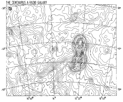
In contrast to single dishes, interferometers often have excellent angular resolution (again , but now is the maximum distance between any pair of antennas in the array). However, the field of view is FOV, where is the size of an individual antenna. Thus, the smaller the individual antennas, the larger the field of view, but also the worse the sensitivity. Very large numbers of antennas increase the design cost for the array and the on-line correlator to process the signals from a large number of interferometer pairs. An additional aspect of interferometers is their reduced sensitivity to extended source components, which depends essentially on the smallest distance, say , between two antennas in the interferometer array. This is often called the minimum spacing or shortest baseline. Roughly speaking, source components larger than radians will be attenuated by more than 50% of their flux, and thus practically be lost. Figure 1 gives an extreme example of this, showing two images of the radio galaxy with the largest apparent size in the sky (10∘). It is instructive to compare this with a high-frequency single-dish map in [Junkes et al. (1993)].
The limitation in sensitivity for extended structure is even more severe for Very Long Baseline Interferometry (VLBI) which uses intercontinental baselines providing 10-3 arcsec (1 mas) resolution. The minimum baseline is often several hundred km, making the largest detectable component much smaller than an arcsec.
[McKay & McKay (1998)] created a WWW tool that simulates how radio interferometers
work. This Virtual Radio Interferometer
(VRI; www.jb.man.ac.uk/~dm/vri/)
comes with the “VRI Guide” describing the basic concepts
of radio interferometry. The applet simulates how the placement of
the antennas affects the uv-coverage of a given array and
illustrates the Fourier transform relationship between the
accumulated radio visibilities and the resultant image.
The comparatively low angular resolution of single dish radio telescopes naturally suggests their use at relatively high frequencies. However, at centimetre wavelengths atmospheric effects (e.g. passing clouds) will introduce additional emission or absorption while scanning, leaving a stripy pattern along the scanning direction (so-called “scanning effects”). Rastering the same field along DEC rather than RA, would lead to a pattern perpendicular to the first one. A comparison and subsequent combination of the two maps, either in the real or the Fourier plane, can efficiently suppress these patterns and lead to a sensitive map of the region ([Emerson & Gräve (1988)]).
A further efficient method to reduce atmospheric effects in single-dish radio maps is the so-called “multi-feed technique”. The trick is to use pairs of feeds in the focal plane of a single dish. At any instant each feed receives the emission from a different part of the sky (their angular separation, or “beam throw”, is usually 5–10 beam sizes). Since they largely overlap within the atmosphere, they are affected by virtually the same atmospheric effects, which then cancel out in the difference signal between the two feeds. The resulting map shows a positive and negative image of the same source, but displaced by the beam throw. This can then be converted to a single positive image as described in detail by [Emerson et al. (1979)]. One limitation of the method is that source components larger than a few times the largest beam throw involved will be lost. The method has become so widely used that an entire symposium has been dedicated to it ([Emerson & Payne (1995)]).
From the above it should be clear that single dishes and interferometers actually complement each other well, and in order to map both the small- and large-scale structures of a source it may be necessary to use both. Various methods for combining single-dish and interferometer data have been devised, and examples of results can be found in [Brinks & Shane (1984)], [Landecker et al. (1990)], [Joncas et al. (1992)], Landecker et al. (1992), [Normandeau et al. (1992)] or [Langer et al. (1995)]. The Astronomical Image Processing System (AIPS; www.cv.nrao.edu/aips), a widely used reduction package in radio astronomy, provides the task IMERG (cf. www.cv.nrao.edu/aips/cook.html) for this purpose. The software package Miriad (www.atnf.csiro.au/computing/software/miriad) for reduction of radio interferometry data offers two programs (immerge and mosmem) to realise this combination of single dish and interferometer data (§2.3). The first one works in the Fourier plane and uses the single dish and mosaic data for the short and long spacings, respectively. The second one compares the single dish and mosaic images and finds the “Maximum Entropy” image consistent with both.
2.2 Special Techniques in Radio Interferometry
A multitude of “cosmetic treatments” of interferometer data have been developed, both for the “uv-” or visibility data and for the maps (i.e. before and after the Fourier transform), mostly resulting from 20 years of experience with the most versatile and sensitive radio interferometers currently available, the Very Large Array (VLA) and its more recent VLBI counterparts the European VLBI Network (EVN), and the Very Large Baseline Array (VLBA); see their WWW pages at www.nrao.edu/vla/html/VLAhome.shtml, www.nfra.nl/jive/evn/evn.html, and www.nrao.edu/vlba/html/VLBA.html. The volumes edited by [Perley et al. (1989), Cornwell & Perley (1991)], and [Zensus et al. (1995)] give an excellent introduction to these effects, the procedures for treating them, as well as their limitations. The more prominent topics are bandwidth and time-average smearing, aliasing, tapering, uv-filtering, CLEANing, self-calibration, spectral-line imaging, wide-field imaging, multi-frequency synthesis, etc.
2.3 Mosaicing
One way to extend the field of view of interferometers is to take “snapshots” of several individual fields with adjacent pointing centres (or phase centres) spaced by no further than about one (and preferably half a) “primary beam”, i.e. the HPBW of the individual array element. For sources larger than the primary beam of the single interferometer elements the method recovers interferometer spacings down to about half a dish diameter shorter than those directly measured, while for sources that fit into the primary beam mosaicing (also spelled “mosaicking”) will recover spacings down to half the dish diameter ([Cornwell (1988)], or [Cornwell (1989)]). The data corresponding to shorter spacings can be taken either from other single-dish observations, or from the array itself, using it in a single-dish mode. The “Berkeley Illinois Maryland Association” (BIMA; bima.astro.umd.edu/bima/) has developed a homogeneous array capability, which is the central design issue for the planned NRAO Millimeter Array (MMA; www.mma.nrao.edu/). The strategy involves mosaic observations with the BIMA compact array during a normal 6–8 hour track, coupled with single-antenna observations with all array antennas mapping the same extended field (see [Pound et al. (1997)] or bima.astro.umd.edu:80/bima/memo/memo57.ps).
Approximately 15% of the observing time on the Australia Telescope Compact Array (ATCA; www.narrabri.atnf.csiro.au/) is spent on observing mosaics. A new pointing centre may be observed every 25 seconds, with only a few seconds of this time consumed by slewing and other overheads. The largest mosaic produced on the ATCA by 1997 is a 1344 pointing-centre spectral-line observation of the Large Magellanic Cloud. Joint imaging and deconvolution of this data produced a 19972230120 pixel cube (see www.atnf.csiro.au/research/lmc_h1/). Mosaicing is heavily used in the current large-scale radio surveys like NVSS, FIRST, and WENSS (§3.7).
2.4 Map Interpretation
The dynamic range of a map is usually defined as the ratio of the peak brightness to that of the “lowest reliable brightness level”, or alternatively to that of the rms noise of a source-free region of the image. For both interferometers and single dishes the dynamic range is often limited by sidelobes occurring near strong sources, either due to limited uv-coverage, and/or as part of the diffraction pattern of the antenna. Sometimes the dynamic range, but more often the ratio between the peak brightness of the sidelobe and the peak brightness of the source, is given in dB, this being ten times the decimal logarithm of the ratio. In interferometer maps these sidelobes can usually be reduced using the CLEAN method, although more sophisticated methods are required for the strongest sources (cf. [Noordam & de Bruyn (1982)], [Perley (1989)]), for which dynamic ranges of up to 5105 can be achieved ([de Bruyn & Sijbring (1993)]). For an Alt-Az single dish the sidelobe pattern rotates with time on the sky, so a simple average of maps rastered at different times can reduce the sidelobe level. But again, to achieve dynamic ranges of better than a few thousand the individual scans have to be corrected independently before they can be averaged ([Klein & Mack (1995)]).
Confusion occurs when there is more than one source in the telescope beam. For a beam area , the confusion limit Sc is the flux density at which this happens as one considers fainter and fainter sources. For an integral source count N(S), i.e. the number of sources per sterad brighter than flux density S, the number of sources in a telescope beam is N(S). Sc is then given by N(S1. A radio survey is said to be confusion-limited if the expected minimum detectable flux density Smin is lower than Sc. Clearly, the confusion limit decreases with increasing observing frequency and with smaller telescope beamwidth. Apart from estimating the confusion limit theoretically from source counts obtained with a telescope of much lower confusion level (see [Condon (1974)]), one can also derive the confusion limit empirically by subsequent weighted averaging of N maps with (comparable) noise level , and with each of them not confusion-limited. The weight of each map should be proportional to . In the absence of confusion, the expected noise, , of the average map should then be
If this is confirmed by experiment, we can say that the “confusion noise” is negligible, or at least that . However, if approaches a saturation limit with increasing N, then the confusion noise, , can be estimated according to . As an example, the confusion limit of a 30-m dish at 1.5 GHz (=20 cm) and a beam width of HPBW=34′ is 400 mJy. For a 100-m telescope at 2.7, 5 and 10.7 GHz (=11 cm, 6 cm and 2.8 cm; HPBW=4.4′, 2.5′ and 1.2′), the confusion limits are 2, 0.5, and 0.1 mJy. For the VLA D-array at 1.4 GHz (HPBW=50′′) it is 0.1 mJy. For radio interferometers the confusion noise is generally negligible owing to their high angular resolution, except for deep maps at low frequencies where confusion due to sidelobes becomes significant (e.g. for WENSS and SUMSS, see §3.7). Note the semantic difference between “confusion noise” and “confusion limit”. They can be related by saying that in a confusion-limited survey, point sources can be reliably detected only above the confusion limit, or 2–3 times the confusion noise, while coherent extended structures can be reliably detected down to lower limits, e.g. by convolution of the map to lower angular resolution. There is virtually no confusion limit for polarised intensity, as the polarisation position angles of randomly distributed, faint background sources tend to cancel out any net polarisation (see [Rohlfs & Wilson (1996)], p. 216 for more details). Examples of confusion-limited surveys are the large-scale low frequency surveys e.g. at 408 MHz ([Haslam et al. (1982)]), at 34.5 MHz ([Dwarakanath & Udaya Shankar (1990)]), and at 1.4 GHz ([Condon & Broderick (1986a)]). Of course, confusion becomes even more severe in crowded areas like the Galactic plane ([Kassim (1988)]).
When estimating the error in flux density of sources (or their
significance) several factors have to be taken into account.
The error in absolute calibration, , depends on the
accuracy of the adopted flux density scale and is usually of the order
of a few per cent. Suitable absolute calibration sources for single-dish
observations are listed in [Baars et al. (1977)] and
[Ott et al. (1994)] for intermediate frequencies,
and in [Rees (1990a)] for low frequencies. Note that
for the southern hemisphere older flux scales are still in use, e.g. [Wills (1975)].
Lists of calibrator sources for intermediate-resolution interferometric
observations (such as the VLA) can be found at the URL
www.nrao.edu/~gtaylor/calib.html, and those for very-high
resolution observations (such as the VLBA) at
magnolia.nrao.edu/vlba_calib/vlbaCalib.txt.
When comparing different source lists it is important to note that,
especially at frequencies below 400 MHz, there are still different
“flux scales” being used which may differ by 10%,
and even more below 100 MHz.
The “zero-level error” is important mainly for single-dish
maps and is given by =/,
where is the number of beam areas contained in the source integration area,
is the number of beam areas in the area of noise determination, and
is the noise level determined in regions “free of emission”
(and includes contributions from the receiver, the atmosphere,
and confusion). The error due to noise in the integration area
is .
The three errors combine to give a total flux density error of
([Klein & Emerson (1981)]).
Clearly, the relative error grows with the extent of a source. This also
implies that the upper limit to the flux density of a non-detected source
depends on the size assumed for it : while a point source of ten times the
noise level will clearly be detected, a source of the same flux, but
extending over many antenna beams may well remain undetected.
In interferometer observations the non-zero size of the shortest baseline
limits the sensitivity to extended sources.
At frequencies 10 GHz the atmospheric absorption starts to
become important, and the measured flux S will depend on elevation
approximately according
to SS∘ exp( csc ),
where S∘ is the extra-atmospheric flux density, and the
optical depth of the atmosphere.
E.g., at 10.7 GHz and at sea level, typical values of are
0.05–0.10, i.e. 5–10% of the flux is absorbed even
when pointing at the zenith. These increase with frequency, but decrease
with altitude of the observatory.
Uncertainties in the zenith-distance dependence
may well dominate other sources of error above 50 GHz.
When estimating flux densities from interferometer maps, the maps should have been corrected for the polar diagram (or “primary beam”) of the individual antennas, which implies a decreasing sensitivity with increasing distance from the pointing direction. This so-called “primary-beam correction” divides the map by the attenuation factor at each map point and thus raises both the intensity of sources, and the map noise, with increasing distance from the phase centre. Some older source catalogues, mainly obtained with the Westerbork Synthesis Radio Telescope (WSRT; e.g. [Oort & van Langevelde (1987)], or [Righetti et al. (1988)]) give both the (uncorrected) “map flux” and the (primary-beam corrected) “sky flux”. The increasing uncertainty of the exact primary beam shape with distance from the phase centre may dominate the flux density error on the periphery of the field of view.
Care should be taken in the interpretation of structural source parameters in catalogues. Some catalogues list the “map-fitted” source size, , as drawn directly from a Gaussian fit of the map. Others quote the “deconvolved” or “intrinsic” source size, . All of these are model-dependent and usually assume both the source and the telescope beam to be Gaussian (with full-width at half maximum, FWHM=), in which case we have . Values of “0.0” in the size column of catalogues are often found for “unresolved” sources. Rather than zero, the intrinsic size is smaller than a certain fraction of the telescope beam width. The fraction decreases with increasing signal-to-noise (S/N) ratio of the source. Estimation of errors in the structure parameters derived from 2-dimensional radio maps is discussed in [Condon (1997)]. Sometimes flux densities are quoted which are smaller than the error, or even negative (e.g. [Dressel & Condon (1978)], and [Klein et al. (1996)]). These should actually be converted to, and interpreted as upper limits to the flux density.
2.5 Intercomparison of Different Observations and Pitfalls
Two main emission mechanisms are at work in radio sources (e.g. [Pacholczyk (1970)]). The non-thermal synchrotron emission of relativistic electrons gyrating in a magnetic field is responsible for supernova remnants, the jets and lobes of radio galaxies and much of the diffuse emission in spiral galaxies (including ours) and their haloes. The thermal free-free or bremsstrahlung of an ionised gas cloud dominates e.g. in H II regions, planetary nebulae, and in spiral galaxies at high radio frequencies. In addition, individual stars may show “magneto-bremsstrahlung”, which is synchrotron emission from either mildly relativistic electrons (“gyrosynchrotron” emission) or from less relativistic electrons (“cyclotron” or “gyroresonance” emission). The historical confirmation of synchrotron radiation came from the detection of its polarisation. In contrast, thermal radiation is unpolarised, and characterised by a very different spectral shape than that of synchrotron radiation. Thus, in order to distinguish between these mechanisms, multi-frequency comparisons are needed. This is trivial for unresolved sources, but for extended sources care has to be taken to include the entire emission, i.e. integrated over the source area. Peak fluxes or fluxes from high-resolution interferometric observations will usually underestimate their total flux. Very-low frequency observations may overestimate the flux by picking up radiation from neighbouring (or “blending”) sources within their wide telescope beams. Compilations of integrated spectra of large numbers of extragalactic sources have been prepared e.g. by [Kühr et al. (1979)], [Herbig & Readhead (1992)], and [Bursov et al. (1997)] (see cats.sao.ru/cats_spectra.html).
An important diagnostic of the energy transfer within radio sources is a two-dimensional comparison of maps observed at different frequencies. Ideally, with many such frequencies, a spectral fit can be made at each resolution element across the source and parameters like the relativistic electron density and radiation lifetime, magnetic field strength, separation of thermal and non-thermal contribution, etc. can be estimated (cf. [Klein et al. (1989)] or [Katz-Stone & Rudnick (1994)]). However, care must be taken that the observing instruments at the different frequencies were sensitive to the same range of “spatial frequencies” present in the source. Thus interferometer data which are to be compared with single-dish data should be sensitive to components comparable to the entire size of the source. The VLA has a set of antenna configurations with different baseline lengths that can be matched to a subset of observing frequencies in order to record a similar set of spatial frequencies at widely different wavelengths – these are called “scaled arrays”. For example, the B-configuration at 1.4 GHz and the C-configuration at 4.8 GHz form one such pair of arrays. Recent examples of such comparisons for very extended radio galaxies can be found in [Mack et al. (1997)] or [Sijbring & de Bruyn (1998)]. Maps of the spectral indices of Galactic radio emission between 408 and 1420 MHz have even been prepared for the entire northern sky ([Reich & Reich (1988)]). Here the major limitation is the uncertainty in the absolute flux calibration.
2.6 Linear Polarisation of Radio Emission
As explained in G. Miley’s lectures for this winter school, the linear polarisation characteristics of radio emission give us information about the magneto-ionic medium, both within the emitting source and along the line of sight between the source and the telescope. The plane of polarisation (the “polarisation position angle”) will rotate while passing through such media, and the fraction of polarisation (or “polarisation percentage”) will be reduced. This “depolarisation” may occur due to cancellation of different polarisation vectors within the antenna beam, or due to destructive addition of waves having passed through different amounts of this “Faraday” rotation of the plane of polarisation, or also due to significant rotation of polarisation vectors across the bandwidth for sources of high rotation measure (RM). More detailed discussions of the various effects affecting polarised radio radiation can be found in Pacholczyk (1970, 1977), [Gardner et al. (1966)], [Burn (1966)], and [Cioffi & Jones (1980)].
During the reduction of polarisation maps, it is important to estimate the ionospheric contribution to the Faraday rotation, which increases in importance at lower frequencies, and may show large variations at sunrise or sunset. Methods to correct for the ionospheric rotation depend on model assumptions and are not straightforward. E.g., within the AIPS package the “Sunspot” model may be used in the task FARAD. It relies on the mean monthly sunspot number as input, available from the US National Geophysical Data Centre at www.ngdc.noaa.gov/stp/stp.html. The actual numbers are in files available from ftp://ftp.ngdc.noaa.gov/STP/SOLAR_DATA/SUNSPOT_NUMBERS/ (one per year: filenames are year numbers). Ionospheric data have been collected at Boulder, Colorado, up to 1990 and are distributed with the AIPS software, mainly to be used with VLA observations. Starting from 1990, a dual-frequency GPS receiver at the VLA site has been used to estimate ionospheric conditions, but the data are not yet available (contact cflatter@nrao.edu). Raw GPS data are available from ftp://bodhi.jpl.nasa.gov/pub/pro/y1998/ and from ftp://cors.ngs.noaa.gov/rinex/. The AIPS task GPSDL for conversion to total electron content (TEC) and rotation measure (RM) is being adapted to work with these data.
A comparison of polarisation maps at different frequencies allows one to derive two-dimensional maps of RM and depolarisation (DP, the ratio of polarisation percentages between two frequencies). This requires the maps to be sensitive to the same range of spatial frequencies. Generally such comparisons will be meaningful only if the polarisation angle varies linearly with , as it indeed does when using sufficiently high resolution (e.g. [Dreher et al. (1987)]). The law may be used to extrapolate the electric field vector of the radiation to 0. This direction is called the “intrinsic” or “zero-wavelength” polarisation angle (), and the direction of the homogeneous component of the magnetic field at this position is then perpendicular to (for optically thin relativistic plasmas). Even then a careful analysis has to be made as to which part of RM and DP is intrinsic to the source, which is due to a “cocoon” or intracluster medium surrounding the source, and which is due to our own Galaxy. The usual method to estimate the latter contribution is to average the integrated RM of the five or ten extragalactic radio sources nearest in position to the source being studied. Surprisingly, the most complete compilations of RM values of extragalactic radio sources date back many years ([Tabara & Inoue (1980)], [Simard-Normandin et al. (1981)], or [Broten et al. (1988)]).
An example of an overinterpretation of these older low-resolution polarisation data is the recent claim ([Nodland & Ralston (1997)]) that the Universe shows a birefringence for polarised radiation, i.e. a rotation of the polarisation angle not due to any known physical law, and proportional to the cosmological distance of the objects emitting linearly polarised radiation (i.e. radio galaxies and quasars). The analysis was based on 20-year old low-resolution data for integrated linear polarisation ([Clarke et al. (1980)]), and the finding was that the difference angle between the intrinsic (=0) polarisation angle and the major axis of the radio structure of the chosen radio galaxies was increasing with redshift. However, it is now known that the distribution of polarisation angles at the smallest angular scales is very complex, so that the integrated polarisation angle may have little or no relation with the exact orientation of the radio source axis. Although the claim of birefringence has been contested by radio astronomers ([Wardle et al. (1997)]), and more than a handful of contributions about the issue have appeared on the LANL/SISSA preprint server (astro-ph/9704197, 9704263, 9704285, 9705142, 9705243, 9706126, 9707326, 9708114) the original authors continue to defend and refine their statistical methods (astro-ph/9803164). Surprisingly, these articles neither explicitly list the data actually used, nor do they discuss their quality or their appropriateness for the problem (cf. the comments in sect. 7.2 of [Trimble & McFadden (1998)]).
2.7 Cross-Identification Strategies
While the nature of the radio emission can be inferred from the spectral and polarisation characteristics, physical parameters can be derived only if the distance to the source is known. This requires identification of the source with an optical object (or an IR source for very high redshift objects) so that an optical spectrum may be taken and the redshift determined. By adopting a cosmological model, the distance of extragalactic objects can then be inferred. For sources in our own Galaxy kinematical models of spiral structure can be used to estimate the distance from the radial velocity, even without optical information, e.g. using the H I line (§6.4). More indirect estimates can also be used, e.g. emission measures for pulsars, apparent sizes for H I clouds, etc.
The strategies for optical identification of extragalactic radio sources are very varied. The easiest case is when the radio position falls within the optical extent of a galaxy. Also, a detailed radio map of an extended radio galaxy usually suggests the position of the most likely optical counterpart from the symmetry of the radio source. Most often two extended radio lobes straddle a point-like radio core which coincides with the optical object. However, various types of asymmetries may complicate the relation between radio morphology and location of the parent galaxy (see e.g. Figs. 6 and 7 of [Miley (1980)]). These may be wiggles due to precession of the radio jet axis, or bends due to the movement of the radio galaxy through an intracluster medium (see www.jb.man.ac.uk/atlas/icon.html for a fine collection of real maps). For fainter and less extended sources the literature contains many different methods to determine the likelihood of a radio-optical association ([Notni & Fröhlich (1975)], [Richter (1975)], [Padrielli & Conway (1977)], [de Ruiter et al. (1977)]). The last of these papers proposes the dimensionless variable where and are the positional differences between radio and optical position, and and are the combined radio and optical positional errors in RA () and DEC (), respectively. The likelihood ratio, , between the probability for a real association and that of a chance coincidence is then , where , with being the density of optical objects. The value of will depend on the Galactic latitude and the magnitude limit of the optical image. Usually, for small sources, 2 is regarded as sufficient to accept the identification, although the exact threshold is a matter of “taste”. A method that also takes into account also the extent of the radio sources, and those of the sources to be compared with (be it at optical or other wavelengths), has been described in [Hacking et al. (1989)]). A further generalisation to elliptical error boxes, inclined at any position angle (like those of the IRAS satellite), is discussed in [Condon et al. (1995)].
A very crude assessment of the number of chance coincidences from two random sets of and sources distributed all over the sky is chance pairs within an angular separation of less than (in radians). In practice the decision on the maximum acceptable for a true association can be drawn from a histogram of the number of pairs within , as a function of . If there is any correlation between the two sets of objects, the histogram should have a more or less pronounced and narrow peak of true coincidences at small , then fall off with increasing up to a minimum at , before rising again proportional to due to pure chance coincidences. The maximum acceptable is then usually chosen near (cf. [Bischof & Becker (1997)] or [Boller et al. (1998)]). At very faint (sub-mJy) flux levels, radio sources tend to be small (10′′), so that there is virtually no doubt about the optical counterpart, although very deep optical images, preferably from the Hubble Space Telescope (HST), are needed to detect them ([Fomalont et al. (1997)]).
However, the radio morphology of extended radio galaxies may be such that only the two outer “hot spots” are detected without any trace of a connection between them. In such a case only a more sensitive radio map will reveal the position of the true optical counterpart, by detecting either the radio core between these hot spots, or some “radio trails” stretching from the lobes towards the parent galaxy. The paradigm is that radio
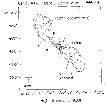
galaxies are generally ellipticals, while spirals only show weak radio emission dominated by the disk, but with occasional contributions from low-power active nuclei (AGN). Recently an unusual exception has been discovered: a disk galaxy hosting a large double-lobed radio source (Figure 2), almost perpendicular to its disk, and several times the optical galaxy size ([Ledlow et al. (1998)]).
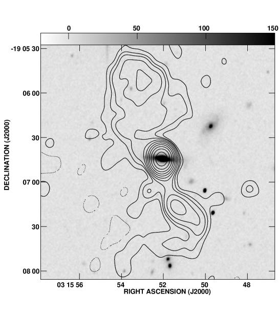
An approach to semi-automated optical identification of radio sources using the Digitized Sky Survey is described in [Haigh et al. (1997)]. However, Figure 3 shows one of the more complicated examples from this paper. Note also that the concentric contours near the centre of the radio source encircle a local minimum, and not a maximum. To avoid such ambiguities some software packages (e.g. “NOD2”, [Haslam (1974)]) produce arrowed contours indicating the direction of the local gradient in the map.
Morphological considerations can sometimes lead to interesting misinterpretations. A linear feature detected in a Galactic plane survey with the Effelsberg 100-m dish had been interpreted as probably being an optically obscured radio galaxy behind our Galaxy ([Seiradakis et al. (1985)]). It was not until five years later ([Landecker et al. (1990)]) that interferometer maps taken with the Dominion Radio Astrophysical Observatory (DRAO; www.drao.nrc.ca) revealed that the linear feature was merely the straighter part of the shell of a weak and extended supernova remnant (G 65.10.6).
One of the most difficult classes of source to identify optically are the so-called “relic” radio sources, typically occurring in clusters of galaxies, with a very steep radio continuum spectrum, and without clear traces of association with any optical galaxy in their host cluster. Examples can be found in [Giovannini et al. (1991)], [Feretti et al. (1997)], or [Röttgering et al. (1997)]. See astro-ph/9805367 for the latest speculation on their origin.
Generally source catalogues are produced only for detections above the 3–5 level. However, [Lewis (1995)] and [Moran et al. (1996)] have shown that a cross-identification between catalogues at different wavelengths allows the “detection” of real sources even down to the 2 level.
3 Radio Continuum Surveys
3.1 Historical Evolution
Our own Galaxy and the Sun were the first cosmic radio sources to be detected due the work of K. Jansky, G. Reber, G. Southworth, and J. Hey in the 1930s and 1940s. Several other regions in the sky had been found to emit strong discrete radio emission, but in these early days the angular resolution of radio telescopes was far too poor to uniquely identify the sources with something “known”, i.e. with an optical object, as there were simply too many of the latter within the error box of the radio position. It was not until 1949 that [Bolton et al. (1949)] identified three further sources with optical objects. They associated Tau A with the “Crab Nebula”, a supernova remnant in our Galaxy, Vir A with M 87, the central galaxy in the Virgo cluster, and Cen A with NGC 5128, a bright nearby elliptical galaxy with a prominent dust lane. By 1955, with the publication of the “2C” survey ([Shakeshaft et al. (1955)]) the majority of radio sources were still thought to be Galactic stars, albeit faint ones, since no correlation with bright stars was observed. However, in the previous year, the bright radio source Cyg A had been identified with a very faint (16m) and distant (z=0.057) optical galaxy ([Baade & Minkowski (1954)]).
Excellent accounts of early radio astronomy can be found in the volumes by Hey (1971, 1973), [Graham-Smith (1974), Edge & Mulkay (1976)], [Sullivan III (1982)], Sullivan III (1984), [Kellermann & Sheets (1984), Robertson (1992)], and in [Haynes et al. (1996)], the latter two describing the Australian point of view. The growth in the number of discrete source lists from 1946 to the late 1960s is given in Appendix 4 of [Pacholczyk (1970)]. Many of the major source surveys carried out during the late 1970s and early 1980s (6C, UTR, TXS, B2, MRC, WSRT, GB, PKS, S1–S5) are described in [Jauncey (1977)]. The proceedings volume by [Condon & Lockman (1990)] includes descriptions of several large-scale surveys in the continuum, H I, recombination lines, and searches for pulsars and variable sources.
3.2 Radio Source Nomenclature : The Good, the Bad and the Ugly
As an aside, Appendix 4 of [Pacholczyk (1970)] explains the difficulty (and liberty!) with which radio sources were designated originally. In the early 1950s, with only a few dozen radio sources known, one could still afford to name them after the constellation in which they were located followed by an upper case letter in alphabetic sequence, to distinguish between sources in the same constellation. This method was abandoned before even a couple of sources received the letter B. Curiously, even in 1991, the source PKS B1343601 was suggested a posteriori to be named “Cen B” as it is the second strongest source in Centaurus ([McAdam (1991)]). Apparently the name has been adopted (see [Tashiro et al. (1998)]). Sequential numbers like 3C NNN were used in the late 1950s and early 1960s, sorting the sources in RA (of a given equinox, like B1950 at that time and until rather recently). But when the numbers exceeded a few thousand, with the 4C survey ([Pilkington & Scott (1965)] and [Gower et al. (1967)]) a naming like 4C DD.NN was introduced, where DD indicates the declination strip in which the source was detected and NN is a sequence number increasing with RA of the source, thus giving a rough idea of the source location (although the total number of sources in one strip obviously depends on the declination). A real breakthrough in naming was made with the Parkes (PKS) catalogue ([Bolton et al. (1964)]) where the “IAU convention” of coordinate-based names was introduced. Thus e.g. a name PKS 1234239 would imply that the source lies in the range RA= 12h34m…12h35m and DEC=23∘ 54′…24∘ 0′. Note that to construct the source name the exact position of the source is truncated, not rounded. An even number of digits for RA or DEC would indicate integer hours, minutes or seconds (respectively of time and arc), while odd numbers of digits would indicate the truncated (i.e. downward-rounded) tenth of the unit of the preceding pair of digits. Since the coordinates are equinox-dependent and virtually all previous coordinate-based names were based on B1950, it has become obligatory to precede the coordinate-based name with the letter J if they are based on the J2000 equinox. Thus e.g. PKS B0000506 is the same as PKS J00025024, and the additional digit in DEC merely reflects the need for more precision nowadays. Vice versa, the lack of a fourth digit in the B1950 name reflects the recommendation to never change a name of a source even if its position becomes better known later. The current sensitivity of surveys and the resulting surface density of sources implies much longer names to be unique. Examples are NVSS B102023+252903 or FIRST J102310.0+251352 (which are actually the same source!). Authors should follow IAU recommendations for object names (§8.8). The origin of existing names, their acronyms and recommended formats can be traced with the on-line “Dictionary of Nomenclature of Celestial Objects” (vizier.u-strasbg.fr/cgi-bin/Dic; [Lortet et al. (1994)]). A query for the word “radio” (option “Related to words”) will display the whole variety of naming systems used in radio astronomy, and will yield what is perhaps the most complete list of radio source literature available from a single WWW site. Authors of future radio source lists, and project leaders of large-scale surveys, are encouraged to consult the latter URL and register a suitable acronym for their survey well in advance of publication, so as to guarantee its uniqueness, which is important for its future recognition in public databases.
3.3 Major Radio Surveys
Radio surveys may be categorised into imaging and discrete source surveys. Imaging surveys were mostly done with single dishes and were dedicated to mapping the extended emission of our Galaxy (e.g. [Haslam et al. (1982)], [Dwarakanath & Udaya Shankar (1990)]) or just the Galactic plane ([Reich et al. (1984)], [Jonas et al. (1985)]). Only some of them are useful for extracting lists of discrete sources (e.g. [Reich et al. (1997)]). The semi-automatic procedure of source extraction implies that the derived catalogues are usually limited to sources with a size of at most a few beamwidths of the survey. The highest-resolution radio imaging survey covering the full sky, and containing Galactic foreground emission on all scales, is still the 408 MHz survey ([Haslam et al. (1982)]) with HPBW50′. Four telescopes were used and it has taken 15 years from the first observations to its publication. Its 1.4 GHz counterpart in the northern hemisphere ([Reich (1982)], [Reich & Reich (1986)]) is being completed in the south with data from the 30-m dish at Instituto Argentino de Radioastronomía, Argentina.
The discrete source surveys may be done either with interferometers or with single dishes. Except for the most recent surveys (FIRST, NVSS and WENSS, see §3.7) the interferometer surveys tend to cover only small parts of the sky, typically a single field of view of the array, but often with very high sensitivities reaching a few Jy in the deepest surveys. The source catalogues extracted from discrete source surveys with single dishes depend somewhat on the detection algorithm used to find sources from two-dimensional maps. There are examples where two different source catalogues were published, based on the same original maps. Both the “87GB” ([Gregory & Condon (1991)]) and “BWE” ([Becker et al. (1991)]) catalogues were drawn from the same 4.85 GHz maps ([Condon et al. (1989)]) obtained with the Green Bank 300-ft telescope. The authors of the two catalogues (published on 510 pages of the same volume of ApJS), arrived at 54,579 and 53,522 sources, respectively. While the 87GB gives the peak flux, size and orientation of the source, the BWE gives the integrated flux only, plus a spectral index between 1.4 and 4.85 GHz from a comparison with another catalogue. Thus, while being slightly different, both catalogues complement each other. The same happened in the southern hemisphere, using the same 4.85 GHz receiver on the Parkes 64-m antenna: the “PMN” ([Griffith et al. (1994)]) and “PMNM” catalogues ([Gregory et al. (1994)]) were constructed from the same underlying raw scan data, but using different source extraction algorithms, as well as imposing different limits in both signal-to-noise for catalogue source detection, and in the maximum source size. The larger size limit for sources listed in the PMN catalogue, as compared to the northern 87GB, becomes obvious in an all-sky plot of sources from both catalogues : the Galactic plane is visible only in the southern hemisphere ([Tasker & Wright (1993)]), simply due to the large number of extended sources near the plane which have been discarded in the northern catalogues ([Becker et al. (1991)]). [Baleisis et al. (1998)] have also found a 2%–8% mismatch between 87GB and PMN. Eventually, a further coverage of the northern sky made in 1986 (not available as a separate paper) has been averaged with the 1987 maps (which were the basis for 87GB) to yield the more sensitive GB6 catalogue ([Gregory et al. (1996)]). Thus, a significant difference in source peak flux density between 87GB and GB6 may indicate variability, and [Gregory et al. (1998)] have indeed confirmed over 1400 variables.
If single-dish survey maps (or raster scans) are sufficiently large, they may be used to reveal the structure of Galactic foreground emission and discrete features like e.g. the “loops” or “spurs” embedded in this emission. These are thought to be nearby supernova remnants, an idea supported by additional evidence from X-rays (Egger & Aschenbach 1995) and older polarisation surveys ([Salter (1983)]). Surveys of the linear polarisation of Galactic emission will not be dealt with here. As pointed out by [Salter & Brown (1988)], an all-sky survey of linear polarisation, at a consistent resolution and frequency, is still badly needed. No major polarisation surveys have been published since the compendium of [Brouw & Spoelstra (1976)], except for small parts of the Galactic plane ([Junkes et al. (1987)]). This is analogous to a lack of recent surveys for discrete source polarisation (§2.6). Apart from helping to discern thermal from non-thermal features, polarisation maps have led to the discovery of surprising features which are not present in the total intensity maps ([Wieringa et al. (1993b)], [Gray et al. (1998)]). Although the NVSS (§3.7) is not suitable to map the Galactic foreground emission and its polarisation, it offers linear polarisation data for 2 million radio sources. Many thousands of them will have sufficient polarisation fractions to be followed up at other frequencies, and to study their Faraday rotation and depolarisation behaviour.
3.4 Surveys from Low to High Frequencies: Coverage and Content
There is no concise list of all radio surveys ever made. Purton & Durrell (1991) used 233 different articles on radio source surveys, published 1954–1991, to prepare a list of 386 distinct regions of sky covered by these surveys (cats.sao.ru/doc/SURSEARCH.html). While the source lists themselves were not available to these authors, the list was the basis for a software allowing queries to determine which surveys cover a given region of sky. A method to retrieve references to radio surveys by acronym has been mentioned in §3.2. In §4.1 a quantitative summary is given of what is available electronically.
In this section I shall present the “peak of the iceberg”: in Table 1, I have listed the largest surveys of discrete radio sources which have led to source catalogues available in electronic form. The list is sorted by frequency band (col. 1), and the emphasis is on finder surveys with more than 800 sources and more than 0.3 sources/deg2. However, some other surveys were included if they constitute a significant contribution to our knowledge of the source population at a given frequency, like e.g. re-observations of sources originally found at other frequencies. It is supposedly complete for source catalogues with 2000 entries, whereas below that limit a few source lists may be missing for not fulfilling the above criteria. Further columns give the acronym of the survey or observing instrument, the year(s) of publication, the approximate range of RA and DEC covered (or Galactic longitude l and latitude b for Galactic plane surveys), the angular resolution in arcmin, the approximate limiting flux density in mJy, the total number of sources listed in the catalogue, the average surface density of sources per square degree, and a reference number which is resolved into its “bibcode” in the Notes to the table. Three famous series of surveys are excluded from Table 1, as they are not contiguous large-area surveys, but are dedicated to many individual fields, either for Galactic or for cosmological studies (e.g. source counts at faint flux levels). These are the source lists from various individual pointings of the interferometers at DRAO Penticton (P), Westerbork (W) and the Cambridge One-Mile telescope (5C).
Both single-dish and interferometer surveys are included in Table 1. While interferometers usually provide much higher absolute positional accuracy, there is one major interferometer survey (TXS at 365 MHz; [Douglas et al. (1996)], utrao.as.utexas.edu/txs.html), for which one fifth of its 67,000 catalogued source positions suffer from possible “lobe-shifts”. These sources have a certain likelihood to be located at an alternative, but precisely determined position, about 1′ from the listed position. It is not clear a priori which of the two positions is the true one, but the ambiguity can usually be solved by comparison with other sufficiently high resolution maps (see Fig. B1 of [Vessey & Green (1998)] for an example). For a reliable cross-identification with other catalogues these alternative positions obviously have to be taken into account.
Table 1. Major Surveys of Discrete Radio Sources
Freq Name Year RA(h) Decl(deg) HPBW S_min N of n/ Ref Electr
(MHz) of publ or l(d) or b(d) (’) (mJy) objects sq.deg Status
10-25 UTR-2  78-95    0-24     > -13      25-60 10000    1754   0.2   54  A C
  31  NEK     88   350<l<250  |b|<~2.5   13x 11  4000     703   0.7   51  A C
  38  8C     90/95    0-24     > +60       4.5   1000    5859   1.7    1  A C n
  80# CUL1   73/95    0-24    -48,+35      3.7   2000     999   0.04  41  A C
  80# CUL2   73/95    0-24    -48,+35      3.7   2000    1748   0.06  42  A C
  82  IPS     87      0-24    -10,+83    27x350   500    1789   0.08  52    C
 151  6CI     85      0-24     > +80       4.5    200    1761   5.7    2  A C
 151  6CII    88    8.5-17.5  +30,+51      4.5    200    8278   4.1    3  A C
 151  6CIII   90    5.5-18.3  +48,+68      4.5    200    8749   4.5    4  A C
 151  6CIV    91      0-24    +67,+82      4.5    200    5421   3.8   28  A C
 151  6CVa    93    1.6- 6.2  +48,+68      4.5   ~300    2229   3.0   39  A C
 151  6CVb    93   17.3-20.4  +48,+68      4.5   ~300    1229   2.6   39  A C
 151  6CVI    93   22.6- 9.1  +30,+51      4.5   ~300    6752   2.7   40  A C
 151* 7CI     90   (10.5+41)  (6.5+45)     1.2     80    4723   9.7   21    C
 151  7CII    95     15-19    +54,+76      1.2   ~100    2702   6.5   49  A C n
 151  7CIII   96      9-16    +20,+35      1.2   ~150    5526   4.0   56  A C N
 151  7C(G)   98   80<l<180   |b|<5.5      1.2   ~100    6262   4.8   55    C n
 160# CUL3   77/95    0-24    -48,+35      1.9   1200    2045   0.08  43  A C
 178  4C     65/67    0-24     -7,+80    ~23.    2000    4844   0.2   57  A C N M
 232  MIYUN   96      0-24    +30,+90      3.8   ~100   34426   3.3   24  A C
 325  WENSS  97/98    0-24    +30,+90      0.9     18  229420  ~22.   58    C
 327* WSRT   91/93  5 fields (+40,+72)    ~1.0      3    4157  ~50.   32  A C
 327  WSRTGP  96    43<l<91   |b|<1.6     ~1.0    ~10    3984  ~25.   30  A C n
 365  UTRAO36 92      0-24    +31,+41     ~0.1    250    3196   ~2.   38    C
 365  TXS     96      0-24   -35.5,+71.5  ~0.1    250   66841   ~2.   22  A C n
 408  MRC    81/91    0-24    -85,+18.5   ~3.     700   12141   0.5    6  A C N
 408  B2     70-74    0-24    +24,+40     3 x10   250    9929   3.1    7  A C   M
 408  B3      85      0-24    +37,+47     3 x 5   100   13354   5.2    8  A C N
 408  MC1     73      1-17    -22,-19      2.7    100    1545   2.3    9  A C   M
 408  MC4     76      0-18    -74,-62      2.7    130    1257   1.0   10  A C   M
 408  MDS2    84      5-23    -21,-20      2.8     60     799   2.7   11    C
 611  NAIC    75     22-13     -3,+19     12.6    350    3122   0.6   12    C
 608* WSRT   91/93 sev.fields (~40,~72)    0.5      3    1693  ~50.   32  A C
1400  GB      72      7-16    +46,+52    10 x11    90    1086   2.0   13    C
1400  GB2     78      7-17    +32,+40    10 x11    90    2022   2.2   14    C
1400  WB92    92      0-24     -5,+82    10 x11  ~150   31524   0.7   27  A C N
1400  GPSR    90    20<l<120  |b|<0.8      0.08    25    1992   8.9   33  A C
1400  NVSS34  98     0-24    -40,+90       0.9    2.0 1807317  ~55.   60    C
1400  FIRST5  98   7.3,17.4  +22.2,57.6    0.1    1.0  382892  ~90.   59  A C
1400  FIRST5  98   21.3,3.3  -11.5,+1.6    0.1    1.0   54537  ~90.   59  A C
1408  RRF     90   357<l<95.5  |b|<4.0     9.4     98     884   1.1   29  A C
1420  RRF     98   95.5<l<240 -4<|b|<+5    9.4     80    1830   1.5   44  A C
1420* PDF     98   B0112-46   r=1deg       0.1     0.1   1079  ~340.  62    C
1400  ELAISR  98   3 fields   +32,+55      0.25   0.14    867   205.  61    C
1400  GPSR    92   350<l<40   |b|<1.8      0.08    25    1457   8.1   37    C
1500  VLANEP  94   17.4,18.5  63.6,70.4    0.25   0.5    2436  83.    47  A C n
2700  PKS    (90)     0-24    -90,+27     ~8.     ~50    8264   0.3   15  A C N M
2700  F3R     90   357<l<240   |b|< 5      4.3     40    6483   2.7   34  A C
3900  Z       89      0-24     0,+14     1.2x52    50    8503   1.7   16  A C
3900  Z2      91      0-24     0,+14     1.2x52    40    2944   0.6    5  A C
3900  RC     91-93    0-24     4.5,5.5   1.2x52     4    1189   3.2   26    C n
4775# NAIC-GB 83    22.3-13   -3,+19       2.8    ~20    2661   0.6   17    C
4760  GBdeep  86      0-24      ~33        2.8     15     882   6.6   18    C
4850  MG1-4  86-91    var.   -0.5,+51      2.8     40   24180   1.5   20    C n
4850  87GB    91      0-24     0,+75      ~3.5     25   54579   2.7   19  A C N
4850  BWE     91      0-24     0,+75      ~3.5     25   53522   2.7   23  A C N
4850  GB6     96      0-24     0,+75      ~3.5     18   75162   3.7   53  A C
4850  PMNM    94      0-24    -88,-37      4.9     25   15045   1.8   45  A C N
4850  PMN-S   94      0-24   -87.5,-37     4.2     20   23277   2.8   31a A C N
4850  PMN-T   94      0-24    -29,-9.5     4.2     42   13363   2.0   31b A C N
4850  PMN-E   95      0-24    -9.5,+10     4.2     40   11774   1.9   48  A C N
4850  PMN-Z   96      0-24    -37,-29      4.2     72    2400   1.1   50  A C N
4875  ADP79   79   357<l< 60   |b|<1       2.6   ~120    1186   9.4   25    C
5000  HCS79   79   190<l< 40   |b|<2       4.1    260     915   1.1   46  A C
5000  GT      86    40<l<220   |b|<2       2.8     70    1274   1.8   35    C
5000  GPSR    94   350<l< 40   |b|<0.4    ~0.07     3    1272  26.    36  A C
A total of 66 surveys are listed with altogether 3,058,035 entries.
See the explanations and references in the Notes to this Table.
References and Notes to Table 1
 1a 1995MNRAS.274..447Hales+         | 29  1990A&AS...83..539Reich W.+
 1b 1990MNRAS.244..233Rees           | 30  1996ApJS..107..239Taylor+
 2  1985MNRAS.217..717Baldwin+       | 31a 1994ApJS...91..111Wright+
 3  1988MNRAS.234..919Hales+         | 31b 1994ApJS...90..179Griffith+
 4  1990MNRAS.246..256Hales+         | 32  1993BICDS..43...17Wieringa +PhD Leiden
 5  1991SoSAO..68...14Larionov+      | 33  1990ApJS...74..181Zoonematkermani+
 6a 1991Obs...111...72Large+         | 34  1990A&AS...85..805Fuerst+
 6b 1981MNRAS.194..693Large+         | 35  1986AJ.....92..371Gregory & Taylor
 7a 1970A&AS....1..281Colla+         | 36  1994ApJS...91..347Becker+
 7b 1972A&AS....7....1Colla+         | 37  1992ApJS...80..211Helfand+
 7c 1973A&AS...11..291Colla+         | 38  1992ApJS...82....1Bozyan+
 7d 1974A&AS...18..147Fanti+         | 39  1993MNRAS.262.1057Hales+
 8  1985A&AS...59..255Ficarra+       | 40  1993MNRAS.263...25Hales+
 9  1973AuJPA..28....1Davies+        | 41a 1973AuJPA..27....1Slee & Higgins
10  1976AuJPA..40....1Clarke+        | 41b 1995AuJPh..48..143Slee
11  1984PASAu...5..290White          | 42a 1975AuJPA..36....1Slee & Higgins
12  1975NAICR..45.....Durdin+        | 42b 1995AuJPh..48..143Slee
      NAIC Internal Report           | 43a 1977AuJPA..43....1Slee
13  1972AcA....22..227Maslowski      | 43b 1995AuJPh..48..143Slee
14  1978AcA....28..367Machalski      | 44  1997A&AS..126..413Reich, P.+
15  1991PASAu...9..170Otrupcek+Wright| 45a 1994ApJS...90..173Gregory+
16  1989MIRpubl.......Amirkhanyan+   | 45b 1993AJ....106.1095Condon+
      MIR Publ., Moscow              | 46  1979AuJPA..48....1Haynes+
17  1983ApJS...51...67Lawrence+      | 47  1994ApJS...93..145Kollgaard+
18  1986A&AS...65..267Altschuler     | 48  1995ApJS...97..347Griffith+
19  1991ApJS...75.1011Gregory+Condon | 49  1995A&AS..110..419Visser+
20a 1986ApJS...61....1Bennett+       | 50  1996ApJS..103..145Wright+
20b 1990ApJS...72..621Langston+      | 51  1988ApJS...68..715Kassim
20c 1990ApJS...74..129Griffith+      | 52  1987MNRAS.229..589Purvis+
20d 1991ApJS...75..801Griffith+      | 53  1996ApJS..103..427Gregory+
21  1990MNRAS.246..110McGilchrist+   | 54  1995Ap&SS.226..245Braude+ +older refs
22  1996AJ....111.1945Douglas+       | 55  1998MNRAS.294..607Vessey & Green D.A.
23  1991ApJS...75....1Becker+        | 56  1996MNRAS.282..779Waldram+
24  1997A&AS..121...59Zhang+         | 57a 1965MmRAS..69..183Pilkington & Scott
25  1979A&AS...35...23Altenhoff+     | 57b 1967MmRAS..71...49Gower+
26a 1991A&AS...87....1Parijskij+     | 58  1997A&AS..124..259Rengelink+ and WWW
26b 1992A&AS...96..583Parijskij+     | 59  1997ApJ...475..479White+  and WWW
26c 1993A&AS...98..391Parijskij+     | 60  1998AJ....115.1693Condon+ and WWW
27  1992ApJS...79..331White & Becker | 61  1998MNRAS... Ciliegi+ astro-ph/9805353
28  1991MNRAS.251...46Hales+         | 62  1998MNRAS.296..839Hopkins+ +PhD Sydney
Notes to Table 1. #: not a finder survey, but re-observations of previously catalogued sources. *: circular field, central coordinates and radius are given. The catalogue electronic status is coded as follows : A: available from ADC/CDS (§4.1); C: (all of them!) searchable simultaneously via CATS (§4.2); N: fluxes are in NED; n: source positions are in NED (cf. §4.3); M: included in MSL (§4.1). An update of this table is kept at cats.sao.ru/doc/MAJOR_CATS.html.
The angular resolution of the surveys tends to increase with observing frequency, while the lowest flux density detected tends to decrease (but increase again above 8 GHz). In fact, until recently the relation between observing frequency, , and limiting flux density, , of large-scale surveys between 10 MHz and 5 GHz followed rather closely the power-law spectrum of an average extragalactic radio source, . This implied a certain bias against the detection of sources with rare spectra, like e.g. the “compact steep spectrum” (CSS) or the “GHz-peaked spectrum” (GPS) sources ([O’Dea (1998)]). With the new, deep, large-scale radio surveys like WENSS, NVSS and FIRST (§3.7), with a sensitivity of 10–50 times better than previous ones, one should be able to construct much larger samples of these cosmologically important type of sources (cf. [Snellen et al. (1996)]). A taste of some cosmological applications possible with these new radio surveys has been given in the proceedings volume by [Bremer et al. (1998)].
Table 1 also shows that there are no appreciable source surveys at frequencies higher than 5 GHz, mainly for technical reasons: it takes large amounts of telescope time to cover a large area of sky to a reasonably low flux limit with a comparatively small beam. New receiver technology as well as new scanning techniques will be needed. For example, by continuously (and slowly) slewing with all elements of an array like the VLA, an adequately dense grid of phase centres for mosaicing could be simulated using an appropriate integration time. More probably, the largest gain in knowledge about the mm-wave radio sky will come from the imminent space missions for microwave background studies, MAP and PLANCK (see §8.3). Currently there is no pressing evidence for “new” source populations dominating at mm waves (cf. sect. 3.3 of [Condon et al. (1995)]), although some examples among weaker sources were found recently ([Crawford et al. (1996)], [Cooray et al. (1998)]). Surveys at frequencies well above 5 GHz are thus important to quantify how such sources would affect the interpretation of the fluctuations of the microwave background. Until now, these estimates rely on mere extrapolations of source spectra at lower frequencies, and certainly the information content of the surveys in Table 1 has not at all been fully exploited for this purpose.
Table 1 is an updated version of an earlier one ([Andernach (1992)]) which listed 38 surveys with 450,000 entries. In 1992 I speculated that by 2000 the number of measured flux densities would have quadrupled. The current number (in 1998!) is already seven times the number for 1992.
3.5 Optical Identification Content
The current information on sources within our Galaxy is summarized in §3.6. The vast majority of radio sources more than a few degrees away from the Galactic plane are extragalactic. The latest compilation of optical identifications of extragalactic radio sources dates back to 1983 ([Véron-Cetty & Véron (1983)], hereafter VV83) and lists 14,585 entries for 10,173 different sources, based on 917 publications. About 25% of these are listed as “empty”, “blank” or “obscured” fields (EF, BF, or OF), i.e. no optical counterpart has been found to the limits of detection. The VV83 compilation has not been updated since 1983, and is not to be confused with the “Catalogue of Quasars and Active Galactic Nuclei” by the same authors. Both compilations are sometimes referred to as the (“well-known”) “Véron catalogue”, but usually the latter is meant, and only the latter is being updated ([Véron-Cetty & Véron (1998)] or “VV98”). The only other (partial) effort of a compilation similar to VV83 was PKSCAT90 ([Otrupcek & Wright (1991)]), which was restricted to the 8 263 fairly strong PKS radio sources and, contrary to initial plans, has not been updated since 1990. It also lacks quite a few references published before 1990.
For how many radio sources do we know an optical counterpart ?
From Table 1 we may very crudely estimate that currently well over
2 million radio sources are known (3.3 million individual measurements
are available electronically). A compilation of references
(not included in VV83) on optical identifications of
radio sources maintained by the present author currently holds
560 references dealing with a total of 56,000 objects.
This leads the author to estimate that an optical identification (or absence thereof)
has been reported for 20–40,000 sources. Note that probably
quite a few of these will either occur in more than one reference or
be empty fields. Most of the information contained in VV83 is absent
from pertinent object databases (§4.3), given that these
started including extragalactic data only since 1983
(SIMBAD) and 1988 (NED). However, most of the optical identifications
published since 1988 can be found in NED. Moreover, numerous
optical identifications of radio sources have been made quietly
(i.e. outside any explicit publication) by the NED team. Currently
(May 98) NED contains 9,800 extragalactic objects which are
also radio sources. Only 57% of these have a redshift in NED.
Even if we add to this some 2–3,000 optically identified Galactic
sources (§3.6) we can state fairly safely that
of all known radio sources, we currently know the optical counterpart
for at most half a percent, and the distance for no more
than a quarter percent.
The number of counterparts is likely to increase by thousands
once the new large radio survey catalogues (WENSS, NVSS, FIRST),
as well as new optical galaxy catalogues, e.g. from APM
(www.ast.cam.ac.uk/~apmcat), SuperCOSMOS
(www.roe.ac.uk/scosmos.html) or SDSS (§3.7.3),
become available. Clearly, more automated
identification methods and multifibre spectroscopy (like e.g. 2dF,
FLAIR, and 6dF, all available from www.aao.gov.au/)
will be the only way to reduce the growing gap between the number of
catalogued sources and the knowledge about their counterparts.
3.6 Galactic Plane Surveys and Galactic Sources
Some of the major discrete source surveys of the Galactic plane are included in Table 1 (those for which a range in l and b are listed in columns 4 and 5, and several others covering the plane). Lists of “high”-resolution surveys of the Galactic radio continuum up to 1987 have been given in [Kassim (1988)] and [Reich (1991)]. Due the high density of sources, many of them with complex structure, the Galactic plane is the most difficult region for the preparation of discrete source catalogues from maps. The often unusual shapes of radio continuum sources have led to designations like the “snake”, the “bedspring” or “tornado”, the “mouse” (cf. [Gray (1994a)]) or a “chimney” ([Normandeau et al. (1996)]). For extractions of images from some of these surveys see §6.3.
What kind of discrete radio sources can be found in our Galaxy ?
Of the 100,000 brightest radio sources in the sky, fewer than 20 are stars.
A compilation of radio observations of 3000 Galactic stars has been
maintained until recently by [Wendker (1995)].
The electronic version is available from ADC/CDS
(catalogue # 2199, §4.1) and includes flux densities for about 800
detected stars and upper limits for the rest.
This compilation is not being updated any more. The most recent
push for the detection of new radio stars has just come from
a cross-identification of the FIRST and NVSS catalogues with star catalogues.
In the FIRST survey region the number of known radio stars has
tripled with a few dozen FIRST detections (S 1 mJy at 1.4 GHz,
[Helfand et al. (1997)]), and 50 (mostly new) radio stars were found
in the NVSS ([Condon et al. (1997)]), many of them radio variable.
A very complete WWW page on Supernovae (Sne), including
SNRs, is offered by Marcos J. Montes at
cssa.stanford.edu/~marcos/sne.html.
It provides links to other supernova-related pages, to catalogues of SNe
and SNR, to individual researchers, as well as preprints, meetings and
proceedings on the subject.
D.A. Green maintains his
“Catalogue of Galactic Supernova Remnants”
at www.mrao.cam.ac.uk/surveys/snrs/.
The catalogue contains details of confirmed Galactic SNRs (almost all
are radio SNRs), and includes bibliographic references, together with lists
of other possible and probable Galactic SNRs. From a Galactic plane survey
with the RATAN-600 telescope ([Trushkin (1996)]) S. Trushkin
derived radio profiles along RA at 3.9, 7.7, and 11.1 GHz for 70 SNRs
at cats.sao.ru/doc/Atlas_snr.html
(cf. [Trushkin (1996)]). Radio continuum spectra
for 192 of the 215 SNRs in Green’s catalogue ([Trushkin (1998)]) may be
displayed at cats.sao.ru/cats_spectra.html.
Planetary nebulae (PNe), the expanding shells of stars in a late stage of evolution, all emit free-free radio radiation. The deepest large-scale radio search of PNe has been performed by [Condon & Kaplan (1998)], who cross-identified the “Strasbourg-ESO Catalogue of Galactic Planetary Nebulae” (SESO, available as ADC/CDS # 5084) with the NVSS catalogue. To do this, some of the poorer optical positions in SESO for the 885 PNe north of =40∘ had to be re-measured on the Digitized Sky Survey (DSS; archive.stsci.edu/dss/dss_form.html). The authors detect 680 (77%) PNe brighter than about S(1.4 GHz) = 2.5 mJy/beam. A database of Galactic Planetary Nebulae is maintained at Innsbruck (ast2.uibk.ac.at/). However, the classification of PNe is a tricky subject, as shown by several publications over the past two decades (e.g. [Kohoutek (1997)], [Acker et al. (1991)], or [Acker & Stenholm (1990)]). Thus the presence in a catalogue should not be taken as ultimate proof of its classification.
H II regions are clouds of almost fully ionised hydrogen found
throughout most late-type galaxies. Major compilations of H II regions
in our Galaxy were published by [Sharpless (1959)] (N=313)
and [Marsalkova (1974)] (N=698).
A graphical tool to create charts with objects from 17 catalogues
covering the Galactic Plane, the Milky Way Concordance
(cfa-www.harvard.edu/~peterb/concord),
has already been mentioned in my tutorial in this volume.
Methods to find candidate H II regions based on IR colours
of IRAS Point Sources have been given in [Hughes & MacLeod (1989)] and
Wood & Churchwell (1989), and were further exploited to confirm
ultracompact H II regions (UC H II) via radio continuum observations
([Kurtz et al. (1994)]) or 6.7 GHz methanol maser searches
([Walsh et al. (1997)]). [Kuchar & Clark (1997)] merged six
previous compilations to construct an all-sky list of 1048 Galactic H II
regions, in order to look for radio counterparts in the 87GB and
PMN maps at 4.85 GHz. They detect
about 760 H II regions above the survey threshold of 30 mJy
(87GB) and 60 mJy (PMN). These authors also point out the
very different characteristics of these surveys, the 87GB being much
poorer in extended Galactic plane sources than the PMN, for the reasons
mentioned above (§3.3).
The “Princeton Pulsar Group” (pulsar.princeton.edu/) offers basic explanations of the pulsar phenomenon, a calculator to convert between dispersion measure and distance for user-specified Galactic coordinates, software for analysis of pulsar timing data, links to pulsar researchers, and even audio-versions of the pulses of a few pulsars. The largest catalogue of known pulsars, originally published with 558 records by [Taylor et al. (1993)] is also maintained and searchable there (with currently 706 entries). Pulsars have very steep radio spectra (e.g. [Malofeev (1996)], or astro-ph/9801059, 9805241), are point-like and polarised, so that pulsar candidates can be found from these criteria in large source surveys ([Kouwenhoven et al. (1996)]). Data on pulsars, up to pulse profiles of individual pulsars, from dozens of different papers can be found at the “European Pulsar Network” (www.mpifr-bonn.mpg.de/pulsar/data/). They have developed a flexible data format for exchange of pulsar data ([Lorimer et al. (1998)]), which is now used in an on-line database of pulse profiles as well as an interface for their simultaneous observations of single pulses. The database can be searched by various criteria like equatorial and/or Galactic coordinates, observing frequency, pulsar period and dispersion measure (DM). Further links on radio pulsar resources have been compiled at pulsar.princeton.edu/rpr.shtml, including many recent papers on pulsar research. [Kaplan et al. (1998)] have used the NVSS to search for phase-averaged radio emission from the pulsars north of =40∘ in the [Taylor et al. (1993)] pulsar catalogue. They identify 79 of these pulsars with a flux of S(1.4 GHz) 2.5 mJy, and 15 of them are also in the WENSS source catalogue.
An excellent description of the various types of Galactic radio sources, including masers, is given in several of the chapters of [Verschuur & Kellermann (1988)].
Last, but not least, Galactic plane radio sources can point us to galaxies and clusters in the “Zone of Avoidance” (ZOA). In fact, in a large number of surveys for discrete radio sources, the Galactic plane does not show any excess number density of (usually compact) sources, e.g. in TXS ([Douglas et al. (1996)]) or BWE ([Becker et al. (1991)]). In a 2.7 GHz survey of the region 3∘ 240∘, 5∘, with the Effelsberg 100-m telescope, the density of unresolved sources ( 1′ intrinsic size) was not found to vary with Galactic latitude ([Fürst et al. (1990)]). At much higher resolution (5′′), using the VLA to cover the area 10∘ 40∘, 1.8∘, a concentration of compact sources (size 20′′) towards the Galactic plane becomes noticeable, but only for 0.4∘ ([Helfand et al. (1992)]). [Becker et al. (1994)] have shown that at 5 GHz this distribution has a width of only 10′–15′. Most of the extragalactic sources will be far too optically faint to be ever identified. Two notable counter-examples are the prototype “head-tail” radio source 3C 129 (z=0.021; [Miley et al. (1972)]), now known to be a member of the Perseus supercluster of galaxies ([Hauschildt (1987)]), and “Centaurus B” (see §3.2). Other examples are two tailed radio sources, PKS B1610608 and PKS B1610605 in Abell cluster A 3627, which is thought to be the central clump of the “Great Attractor” ([Kraan-Korteweg et al. (1997)]). A typical wide-angle tailed (WAT) radio source (G 357.3001.24) has been found very close to the Galactic centre, indicating the presence of a cluster of galaxies in that direction ([Gray (1994b)]). Due to the extreme optical obscuration, there is little hope of optically identifying this cluster and determining its distance.
3.7 Modern Large-Scale Discrete Source Surveys: NVSS, FIRST, WENSS and SUMSS
Some of the first large-scale contiguous surveys with interferometers had become available in the 1980s. These were made with arcmin resolution at low frequencies where the large fields of view required only a few pointings (e.g. 6C or 8C; www.mrao.cam.ac.uk/surveys/). Only in the 1990s, however, has the increase in computing power allowed such surveys to be made at even sub-arcmin resolution with the most powerful interferometers like the VLA and the WSRT, requiring up to a quarter of a million pointings. Four ongoing or recently finished surveys in this category are described below.
3.7.1 The “WENSS” Survey at 325–350 MHz
The “Westerbork Northern Sky Survey” (WENSS; www.strw.leidenuniv.nl/wenss) is a radio survey made with the WSRT (www.nfra.nl/wsrt/wsrtpage.htm) from late 1990 to 1996, at frequencies 325 and 610 MHz ( 92 and 49 cm). The entire sky north of declination 30∘ has been covered with 6000 pointings, using a central frequency of 325 MHz below =74∘, and 350 MHz for the polar region. Only 2000 square degrees (20% of the sky north of 30∘) were mapped at 610 MHz, and for the time being only the 325 MHz data have been made available to the public. At 325 MHz the resolution is 5454′′ csc(), and the positional accuracy for strong sources is 1.5′′. The limiting flux density is 18 mJy (5 ) at both frequencies. The final products of WENSS, a 325-MHz atlas of 6∘6∘ maps centred on the new POSS plate positions (5∘ grid) as well as a source catalogue are now available. FITS maps can be drawn from the anonymous ftp server at ftp://vliet.strw.leidenuniv.nl/pub/wenss/HIGHRES/. A postage stamp server for extraction of smaller images is planned for the near future. Also total intensity maps at a lower resolution of 4.2′ will soon be made available. Ionospheric instabilities make the generation of polarisation maps (Stokes Q, U and V) formidably difficult and their production is not currently foreseen.
Presently there are two source catalogues at 325 MHz. The main catalogue contains 211,235 sources for 28∘ 76∘ . The polar catalogue contains 18,341 sources above 74∘ . These can be browsed at the URL www.strw.leidenuniv.nl/wenss/search.html. A detailed description of the survey and the contents of the source lists are given in [Rengelink et al. (1997)].
Due to its low frequency and sensitivity to extended structure the WENSS survey is well-suited to detect very extended or low surface brightness objects like giant radio galaxies (cf. [Schoenmakers et al. (1998)]), cluster haloes, and nearby galaxies. Comparing WENSS with other surveys at higher frequencies allows one to isolate candidates for high-redshift radio galaxies, GHz-peaked spectrum (GPS) sources, flat spectrum sources (e.g. high-redshift quasars), and pulsars.
3.7.2 The “NRAO VLA Sky Survey” at 1.4 GHz (NVSS)
The VLA has been used from 1993 to 1997 to map the entire sky north of =40∘ (82% of the sky) in its most compact (D) configuration, giving an angular resolution of 45′′ at 1.4 GHz. About 220,000 individual snapshots (phase centres) have been observed. They were of a mere 23.5 sec duration each, except at low elevation when they were increased to up to 60 sec to make up for the loss of sensitivity due to ground radiation and air mass. A detailed description is given in [Condon et al. (1998)] (ftp://www.cv.nrao.edu/pub/nvss/paper.ps). The principal data products are:
-
A set of 2326 continuum map “cubes,” 4∘4∘ with images of Stokes parameters I, Q, and U. The noise level is 0.45 mJy/beam in I, and 0.29 mJy/beam in Q and U. Positional accuracy varies from 1′′ for strong (S15 mJy) point sources to 7′′ for the faintest (2.3 mJy) detectable sources.
-
A catalogue of 2,000,000 discrete sources detected in the entire survey
-
Processed uv-data (visibilities) for each map cube constructed from over 100 individual pointings, for users wishing to investigate the data underlying the images.
The NVSS is accessible from www.cv.nrao.edu/~jcondon/nvss.html,
and is virtually complete at the time of writing.
The latest version of the NVSS catalogue (# 34, May 98) is a single
152 Mb FITS file with 1.8106 sources. It can be downloaded via anonymous
ftp, but users interested in exploiting the entire catalogue may
consider requesting a tape copy from NRAO. The publicly available program
NVSSlist can extract selected portions of the catalogue very rapidly
and is easily installed on the user’s local disk
for extensive cross-identification projects.
The catalogue can also be browsed at www.cv.nrao.edu/NVSS/NVSS.html and a “postage stamp server” to extract NVSS images is available at www.cv.nrao.edu/NVSS/postage.html. Images are also available from Skyview (skyview.gsfc.nasa.gov/), but they neither are as up-to-date as those at NRAO, nor do thay have the same FITS header (§6.2). As always, care must be taken in the interpretation of these images. Short integration times and poor uv-coverage can cause grating residuals and limited sensitivity to extended structure (see Fig. 4).
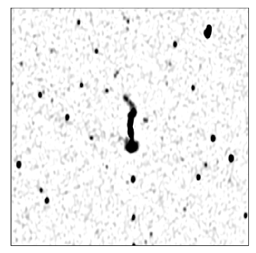
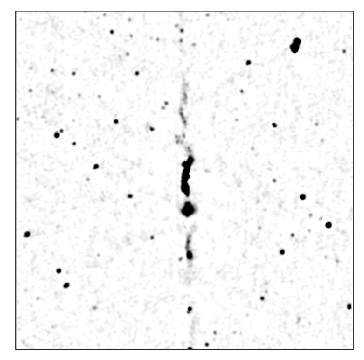
3.7.3 The “FIRST” Survey at 1.4 GHz
The VLA has been used at 1.4 GHz (=21.4 cm) in its B-configuration for another large-scale survey at 5′′ resolution. It is called FIRST (“Faint Images of the Radio Sky at Twenty-centimeters”) and is designed to produce the radio equivalent of the Palomar Observatory Sky Survey over 10,000 square degrees of the North Galactic Cap. An automated mapping pipeline produces images with 1.8′′ pixels and a typical rms noise of 0.15 mJy. At the 1 mJy source detection threshold, there are 90 sources per square degree, about a third of which have resolved structure on scales from 2′′–30′′.
Individual sources have 90% confidence error circles of radius 0.5′′ at the 3 mJy level and 1′′ at the survey threshold. Approximately 15% of the sources have optical counterparts at the limit of the POSS-I plates (E20.0), and unambiguous optical identifications are achievable to m24. The survey area has been chosen to coincide with that of the Sloan Digital Sky Survey (SDSS; www-sdss.fnal.gov:8000/). This area consists mainly of the north Galactic cap (∘) and a smaller region in the south Galactic hemisphere. At the m24 limit of SDSS, about half of the optical counterparts to FIRST sources will be detected.
The homepage of FIRST is sundog.stsci.edu/. By late 1997 the survey had covered about 5000 square degrees. The catalogue of the entire region (with presently 437,000 sources) can be searched interactively at sundog.stsci.edu/cgi-bin/searchfirst. A postage stamp server for FIRST images (presently for 3000 square degrees) is available at third.llnl.gov/cgi-bin/firstcutout. For 1998 and 1999, the FIRST survey was granted enough time to cover an additional 3000 square degrees.
The availability of the full NVSS data products has reduced the enthusiasm of parts of the community to support the finishing of FIRST’s goals. However, only the FIRST survey (and less so the NVSS) provides positions accurate enough for reliable optical identifications, particularly for the cosmologically interesting faint and compact sources. On the other hand, in Figure 5 I have shown an extreme example of the advantage of NVSS for studies of extended sources. In fact, the Figure shows the complementary properties of NVSS and FIRST. A very extended source, perhaps just recognisable with NVSS, will be broken up by FIRST into apparently unrelated components. Thus, it would be worthwhile to look into the feasibility of merging the uv data of NVSS and FIRST to create maps at 10′′–15′′ resolution in the region covered by both surveys.

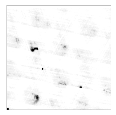
3.7.4 The “SUMSS” 843 MHz Survey with “MOST”
Since 1994 the “Molonglo Observatory Synthesis Telescope” (MOST) has been upgraded from the previous 70′ field of view to a 2.7∘ diameter field of view. As MOST’s aperture is almost filled, the image contains Fourier components with a wide range of angular scales, and has low sidelobes. In mid-1997, the MOST started the “Sydney University Molonglo Sky Survey” (SUMSS; [Hunstead et al. (1998)]). The entire sky south of DEC=30∘ and 10∘ will be mapped at 843 MHz, a total of 8000 square degrees covered by 2713 different 12-h synthesis field centres. It complements northern surveys like WENSS and NVSS, and it overlaps with NVSS in a 10∘ strip in declination (30∘ to 40∘), so as to allow spectral comparisons. SUMSS is effectively a continuation of NVSS to the southern hemisphere (see Table 2). However, with its much better uv coverage it surpasses both WENSS and NVSS in sensitivity to low surface brightness features, and it can fill in some of the “holes” in the uv plane where it overlaps with NVSS. The MOST is also being used to perform a Galactic plane survey (§8).
SUMSS positions are uncertain by no more than 1′′ for sources brighter than 20 mJy, increasing to 2′′ at 10 mJy and 3–5′′ at 5 mJy, so that reliable optical identifications of sources close to the survey limit may be made, at least at high Galactic latitude. In fact, the identification rate on the DSS (§3.6) is 30% down to b22 ([Sadler (1998)]). Observations are made only at night, so the survey rate is 1000 deg2 per year, implying a total period of 8 years for the data collection. The south Galactic cap (30∘) should be completed by mid-2000. The release of the first mosaic images (4∘4∘) is expected for late 1998. The SUMSS team at Univ. Sydney plans to use the NVSS WWW software, so that access to SUMSS will look similar to that for NVSS. For basic information about MOST and SUMSS see www.physics.usyd.edu.au/astrop/SUMSS/.
| WENSS | SUMSS | NVSS | FIRST | |
| Frequency | 325 MHz | 843 MHz | 1400 MHz | 1400 MHz |
| Area (deg2) | 10,100 | 8,000 | 33,700 | 10,000 |
| Resolution (′′) | 45 | 5 | ||
| Detection limit | 15 mJy | 5 mJy | 2.5 mJy | 1.0 mJy |
| Coverage | , | , | ||
| Sources / deg2 | 21 | 40 | 60 | 90 |
| No. of sources | 230,000 | 320,000 | 2,000,000 | 900,000 |
4 Integrated Source Parameters on the Web
In this section I shall describe the resources of information on “integrated” source parameters like position, flux density at one or more frequencies, size, polarisation, spectral index, etc. This information can be found in two distinct ways, either from individual source catalogues, each of which have different formats and types of parameters, or from “object databases” like NED, SIMBAD or LEDA (§4.3). The latter have the advantage of providing a “value-added” service, as they attempt to cross-identify radio sources with known objects in the optical or other wavebands. The disadvantage is that this is a laborious process, implying that radio source catalogues are being integrated at a slow pace, often several years after their publication. In fact, many valuable catalogues and compilations never made it into these databases, and the only way for the user to complement this partial information is to search the available catalogues separately on other servers. Due to my own involvement in providing the latter facilities, I shall briefly review their history.
4.1 The Evolution of Electronic Source Catalogues
Radio astronomers have used electronic equipment from the outset and already needed powerful computers in the 1960s to make radio maps of the sky by Fourier transformation of interferometer visibilities. Surprisingly radio astronomers have not been at the forefront of archiving their results, not even the initially rather small-sized catalogues of radio sources. It is hard to believe that the WSRT maintained one of the earliest electronic and publicly searchable archives of raw interferometer data (see www.nfra.nl/scissor/), but at the same time the source lists of 65 WSRT single-pointing surveys, published from 1973 to 1987 with altogether 8200 sources, had not been kept in electronic form. Instead, 36 of them with a total of 5250 sources were recovered in 1995–97 by the present author, using page-scanners and “Optical Character Recognition” (OCR) techniques.
During the 1970s, R. Dixon at Ohio State Univ. maintained what he called the “Master Source List” (MSL). The first version appeared in print almost 30 years ago ([Dixon (1970)]), and contained 25,000 entries for 12,000 distinct sources. Each entry contained the RA, DEC and flux density of a source at a given observing frequency; any further information published in the original tables was not included. The last version (# 43, Nov. 1981) contained 84,559 entries drawn from 179 references published 1953–1978. The list gives 75,000 distinct source names, but the number of distinct sources is much smaller, though difficult to estimate. It was typed entirely by hand, for which reason it is affected by numerous typing errors ([Andernach (1989)]). Also, it was meant to collect positions and fluxes only from new finder surveys, not to update information on already known sources.
Although the 1980s saw a “renaissance” of radio surveys (e.g. MRC, B3, 6C, MIT-GB, GT, NEK, IPS in Table 1) that decade was a truly “dark age” for radio source databases ([Andernach (1992)]). The MSL, apart from being distributed on tape at cost, was not being updated any more, and by the end of the 1980s there was not a single radio source catalogue among the then over 600 catalogues available from the archives of the two established astronomical data centres, the “Astronomical Data Center” (ADC; adc.gsfc.nasa.gov/adc.html) at NASA-GSFC, and the “Centre de Données astronomiques de Strasbourg” (CDS; cdsweb.u-strasbg.fr/CDS.html). This may explain why even in 1990 the MSL was used to search for high-redshift quasars of low radio luminosity, simply by cross-correlating it with quasar catalogues ([Hutchings et al. (1991)], HDP91 in what follows). These authors (using a version of MSL including data published up to 1975!) noted that the MSL had 23 coincidences within 60′′ from QSOs in the HB 89 compilation ([Hewitt & Burbidge (1989)]) which were not listed as “radio quasars” in HB 89. However, HDP91 failed to note that 13 of these 23 objects were already listed with an optical identification in VV83, published seven years before! From the absence of weak ( 100 mJy) radio sources associated with z 2.5 quasars, HDP91 concluded that there were no high-z quasars of low radio luminosity. However, had the authors used the 1989 edition of VV98 ([Véron-Cetty & Véron (1989)], ADC/CDS # 7126) they would have found about ten quasars weaker than 50 mJy at 5-GHz, from references published before 1989. This would have proven the existence of the objects searched for (but not found) by HDP91 from compilations readily available at that time. The most recent studies by [Bischof & Becker (1997)] and [Hooper et al. (1996)]), however, indicate that these objects are indeed quite rare.
Alerted by this deficiency of publicly available radio source catalogues, I initiated, in late 1989, an email campaign among radio astronomers world-wide. The response from several dozen individuals ([Andernach (1990)]) was generally favourable, and I started to actively collect electronic source catalogues from the authors. By the time of the IAU General Assembly in 1991, I had collected the tabular data from about 40 publications totalling several times the number of records in the MSL. However, it turned out that none of the major radio astronomical institutes was willing to support the idea of a public radio source database with manpower, e.g. to continue the collection effort and prepare the software tools. As a result, the EINSTEIN On-line Service (EINLINE or EOLS), designed to manage X-ray data from the EINSTEIN satellite, offered to serve as a testbed for querying radio source catalogues. Until mid-1993 some 67 source tables with 523,000 entries had been integrated in collaboration with the present author ([Harris et al. (1995)]). These are still searchable simultaneously via a simple telnet session (telnet://einline@einline.harvard.edu). However, in 1994 NASA’s funding of EOLS ceased, and no further catalogues have been integrated since then. A similar service is available from DIRA2 (www.ira.bo.cnr.it/dira/gb/), providing 54 radio catalogues with 2.3 million records, including older versions of the NVSS and FIRST catalogues, as well as many items from the present author’s collection. However, due to lack of manpower, DIRA’s catalogue collection is now outdated, and many items from Table 1 are missing. In late 1993, Alan Wright (ATNF) and the present author produced a stand-alone package (called “COMRAD”) of 12 major radio source catalogues with some 303,600 entries. It comes with dBaseIV search software for PCs and can still be downloaded from URL wwwpks.atnf.csiro.au/databases/surveys/comrad/comrad.html. Several other sites offer more or less “random” and outdated sets of catalogues (a few radio items included) and are less suitable when seeking up-to-date and complete information. Among these are ESO’s STARCAT (arch-http.hq.eso.org/starcat.html), ASTROCAT at CADC (cadcwww.dao.nrc.ca/astrocat), and CURSA within the Starlink project (www.roe.ac.uk/acdwww/cursa/home.html). CURSA is actually designed to be copied to the user’s machine, and to work with local catalogues in a CURSA-compatible format.
From late 1989 until the present, I have continued my activities of collecting source catalogues, and since 1995, I have also employed OCR methods to convert printed source lists into electronic form, among them well-known compilations such as that of [Kühr et al. (1979)] of 250 pages, for which the electronic version had not survived the transition through various storage media. Recovery by OCR requires careful proof-reading, especially for those published in tiny or poorly printed fonts (e.g. Harris & Miley (1978), [Walterbos et al. (1985)], and [Bystedt et al. (1984)]). In many cases the original publications were impossible to recover with OCR. For some of these I had kept preprints (e.g. for [Tabara & Inoue (1980)]) whose larger fonts facilitated the OCR. Numerous other tables (e.g. [Braude et al. (1979)], [Quiniento et al. (1988)] or [Altenhoff et al. (1979)]) were patiently retyped by members of the CATS team (see below). Since about 1996, older source tables are also actively recovered with OCR methods at CDS. Unfortunately, due to poor proof-reading methods, errors are found quite frequently in tables prepared via OCR and released by CDS. Occasionally, tables were prepared independently by two groups, allowing the error rate to be further reduced by inter-comparison of the results. Up to now, radio source tables from 177 articles with a total of 75,000 data records and many thousand lines of text (used as documentation for the tables) were prepared via OCR, mostly by the present author. Surprisingly, about half of the tables (including those received directly from the authors) show some kind of problem (e.g. in nomenclature, internal consistency, or formatting, etc.) that requires attention, before they are able to be integrated into a database or searchable catalogue collection. This shows, unfortunately, that not enough attention is paid to the data section by the referees of papers. While this section may appear uninteresting to them, one should keep in mind that in future re-analyses based on old published data, it is exactly the data section which remains as a heritage to future researchers, and not the interpretations given in the original papers. In the early 1990s, most of the tables were received from the original authors upon request, but currently about half of the tables can be collected from the LANL/SISSA electronic preprint server (xxx.lanl.gov). However, this has the danger that they may not be identical to the actual publication. The vast majority of tabular data sets are received in TeX format, and their conversion to ASCII requires substantial efforts.
Currently my collection of radio source lists
(cats.sao.ru/~cats/doc/Andernach.html) contains
source lists from 500 articles, but only 22% of the tables
are also available from ADC or CDS (§4.2).
While the collection started in 1989, half the 500 data sets were
collected or prepared since 1996, and the current growth rate
is 80 data sets per year. About three dozen further
source lists exist in the CDS archive (§4.2), most of which
are either from the series of nine AAS CDROMs, issued twice a year
from 1994 to 1997 with tables from the ApJ and AJ journals,
or from recent volumes of the A&AS journal, thanks to a 1993 agreement
between the Editors of A&AS and CDS to archive all major
tables of A&AS at the CDS. Unfortunately
such an agreement does not exist with other journals, for which
reason my collection efforts will probably continue until virtually
all astronomical journals provide electronic editions.
Presently some tabular data (e.g. in the electronic A&A)
are offered only as images, while other journals offer only hypertext
versions of their tables, which frequently need further treatment
to be converted to plain ASCII format, required for their
ingestion into databases.
The size distribution of electronic radio source catalogues (including my collection and that of CDS) is plotted in the left panel of Figure 6. For catalogues with more than 200 entries the curve follows a power law with index near , a manifestation of Zipf’s law in bibliometrics ([Nicholls (1987)]). The decline for smaller catalogues is due to the fact that many of them simply do not exist in electronic form. In the right panel of Fig. 6 the growth over time of the cumulative number of records of these catalogues is plotted. The three major increases are due to the MSL in 1981, to the 87GB/GB6/PMN surveys in 1991, and, more recently, to the release of NVSS, FIRST and WENSS in 1996/97.
Already, since the early 1990s, the author’s collection of radio catalogues has been the most comprehensive one stored at a single site. However, the problem of making this heterogeneous set of tables searchable with a common user interface was only solved in 1996, when the author started collaborating with a group of radio astronomers at the Special Astrophysical Observatory (SAO, Russia), who had built such an interface for their “Astrophysical CATalogs support System” (CATS; §4.2). Their common interests in radio astronomy stimulated the ingestion of a large number of items from the collection. By late 1996, CATS had surpassed EOLS in size and scope, and in mid-1997 an email service was opened by CATS, allowing one to query about 200 different source lists simultaneously for any number of user-specified sky positions, with just a single and simple email request.
4.2 Searching in Radio Catalogues: VizieR and CATS
The largest collections of astronomical catalogues, and published tabular data in general, are maintained at the CDS and ADC. The “Astronomer’s Bazaar” at CDS (cdsweb.u-strasbg.fr/Cats.html) has over 2200 catalogues and tables for downloading via anonymous ftp. The full list of items (ftp://cdsarc.u-strasbg.fr/pub/cats/cats.all) may be queried for specific catalogues by author name, keyword, wavelength range, or by name of (space) mission. At NASA’s ADC (adc.gsfc.nasa.gov/adc.html) a similar service exists. Despite the claims that “mirror copies” exist in Japan, India and Russia, CDS and ADC are the only ones keeping their archives current. Both have their own catalogue browsers: VizieR at CDS (vizier.u-strasbg.fr/cgi-bin/VizieR), and Catseye at ADC (tarantella.gsfc.nasa.gov/catseye/ViewerTopPage.html), but currently none of them allows one to query large numbers of catalogues at the same time, although such a system is in preparation within VizieR at the CDS. Presently 200 catalogues appear when VizieR is queried for the waveband “radio”. This includes many lists of H II regions, masers, etc., but excludes many of the major radio continuum surveys listed in Table 1. For radio source catalogues, the CATS system currently has the largest collection, and CATS is definitely preferable when radio continuum data are needed.
The CATS system (cats.sao.ru) currently permits searches through about 200 radio source catalogues from about 150 different references, with altogether over 3 million entries, including current versions of the NVSS, FIRST and WENSS catalogues. Many further radio source lists are available via anonymous FTP, as they have not yet been integrated into the search facility (e.g. when only source names, and not positions, are given in the available electronic version of the catalogue). Documentation is available for most of the source lists, and in many cases even large parts of the original paper text were prepared from page scans.
Catalogues in CATS may be selected individually from cats.sao.ru/cats_search.html, or globally by wavelength range. One may even select all searchable catalogues in CATS (including optical, IR, X-ray), making up over 4 million entries. They may be searched interactively on the WWW, or by sending a batch job via email. To receive the instructions about the exact format for such a batch request, send an empty email to cats@sao.ru (no subject required). The output can be delivered as a homogeneous table of sources from the different catalogues, or each catalogue in its native format. The latter assures that all columns as originally published (but not included in the homogenised table format) may be retrieved, although currently the user has to check the individual catalogue documentation to find out what each column means. With the select option one may retrieve sources from a single sky region, either a rectangle or a circle in different coordinate systems (equatorial B1950 or J2000, or Galactic), while the match option allows a whole list of regions to be searched in order to find all the objects in each region. It is then the responsibility of the user to find out which of these data represent the object (or parts of an object, depending on the telescope characteristics) and may be used for inter-comparisons.
CATS offers a few other useful features. For several multi-frequency radio catalogues (or rather compilations of radio sources) CATS allows radio spectra to be plotted on-the-fly, e.g. for [Kühr et al. (1979)], [Kühr et al. (1981)], ([Otrupcek & Wright (1991)], =PKSCAT90), [Trushkin (1996)], [Kallas & Reich (1980)], [Bursov et al. (1997)]. Various options for fitting these spectra and weighting the individual flux errors are provided. Examples for two sources are shown in Fig. 7. Note that PKSCAT90 includes data obtained at only one epoch per frequency, while the Kühr compilations include several epochs at a given frequency. Therefore the variability of QSO 221603 (=PKS B2216038) becomes obvious only in the lower right panel of Fig. 7.
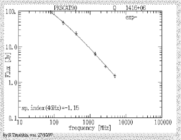
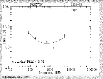
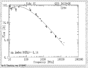
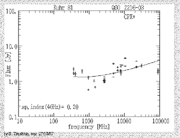
Note that CATS (at least at present) is a searchable collection of catalogues, and not a relational database, i.e. no cross-identifications have yet been made between catalogues (except for a few, which resulted in yet other catalogues). However, given its vastly larger collection of radio source data, it is an indispensable tool that complements the information on radio sources found e.g. in NED or SIMBAD.
In future it is planned that the user may display both the sky distribution and a spectral energy distribution (radio spectrum) of all entries found for a (sufficiently narrow) positional search. The sky plot will indicate the angular resolution, the positional error box, and (if available) the shape of each catalogued source, so that the user may interactively discard possibly unrelated sources, and arrive at the radio spectrum of the object of interest, as mentioned by [Verkhodanov et al. (1997)].
4.3 Object Databases: NED, SIMBAD, and LEDA
These databases have already been described in my tutorial for this winter school, so I shall concentrate here on their relevance for radio astronomy. All three databases were originally built around catalogues of optical objects (galaxies in the case of NED and LEDA, and stars in the case of SIMBAD). It is quite natural that information on otherwise unidentified radio sources is not their priority. Also, being an extragalactic database, NED tends to provide more information on radio sources than SIMBAD, which was originally dedicated to stars, which constitute only a negligible population of radio continuum sources in the sky. The fact that before being included into NED or SIMBAD, every new (radio or other) source has to be checked for its possible identification with another object already in these databases, implies that the integration of large catalogues may take years from their publication. The rightmost column of Table 1 gives an idea of this problem. A further obstacle for database managers is that they have to actively collect the published data from the authors or other resources. If you wish to see your data in databases soonest, the best thing is to send them (preferably in plain ASCII format) to the database managers directly after publication.
SIMBAD is accessible via password from simbad.u-strasbg.fr/Simbad, and has its priority in maintaining a good bibliography for astronomical objects (not necessarily those detected as a radio source only). NED can be accessed freely through the URL nedwww.ipac.caltech.edu and tends to make an effort to also populate its various “data frames” (like optical magnitude, fluxes at various frequencies, etc.) with recently published measurements.
Searches by object name rely on rather strict rules. In databases these may not always conform to IAU recommendations (cdsweb.u-strasbg.fr/iau-spec.html), mainly due to deviations from these recommendations by individual authors. In case of doubt about the exact name of a source, it is wise to start searching the databases by position.
The “Lyon-Meudon Extragalactic Database” (LEDA; www-obs.univ-lyon1.fr/leda) is primarily intended for studying the kinematics of the local Universe, and as such has little interest in radio continuum data on galaxies. However, LEDA is the ideal place to look for integrated neutral hydrogen (H I) data of nearby (z 0.2) galaxies. These H I measurements play an important role for distance estimates of galaxies, independent of their radial velocities. This allows their “peculiar motions” to be calculated, i.e. the deviations of their radial velocities from the Hubble law.
Finally, one should keep in mind that SIMBAD and NED started to include references on extragalactic objects only since 1983 and 1988 respectively, although a few major references before these dates have now been included. In the following I give just one example in which the consequences of this have not been considered by users of NED or SIMBAD. The X-ray source RX J15237+6339 was identified (from NED) with the radio source 4C63.22 by [Brinkmann & Siebert (1994)], and these authors comment that “One object (4C63.22) is classified as ‘Radio Source’ only in the NED data base, so, strictly speaking, it belongs to the class of unidentified objects.” However, according to VV83 (their ref. 603=[Porcas et al. (1980)]) the source 4C63.22 had actually been identified with an 18.5 m galaxy. This object is within 5′′ of the brightest source in the NVSS catalogue within a radius of 90′′. However, the NVSS map shows a large triple radio galaxy with a North-South extent of 4′. Later re-observation at 5 GHz with the VLA at 1.3′′ resolution ([Laurent-Muehleisen et al. (1997)]) detected only a radio core coincident with a 16.6 m object which the 1980 authors had already mentioned in their notes as 1′ offset from their prime candidate identification for the source 1522638. I should add that the data table of the 1980 paper was published on microfiche.
5 Miscellaneous Databases and Surveys of Radio Sources
Several WWW sites offering topical databases of special types of radio source research will be mentioned briefly in this section.
5.1 Clusters of Galaxies
A collection of well-chosen radio source catalogues has been used, together with optical sky surveys like the DSS, to develop a database of radio-optical information on Abell/ACO ([Abell et al. (1989)]) clusters of galaxies. It is managed by A. Gubanov at the St.-Petersburg State University in collaboration with the present author (Gubanov & Andernach 1997). At the URL future.astro.spbu.ru/Clusters.html, the user may interactively prepare schematic radio-optical overlays, charts from the FIRST, NVSS, APM or DSS survey data, or retrieve references for cluster data. Radio continuum spectra of cluster radio galaxies may be displayed and fitted with user-specified functions. Source luminosities may be derived assuming cluster membership.
5.2 VLBI and Astrometric Surveys
The VLBA Calibrator Survey (magnolia.nrao.edu/vlba_calib/) is an ongoing project to provide phase-reference calibrators for VLBA experiments. When completed it will contain astrometric (1 mas) positions and 2.7 and 8.4 GHz images of the 3000 sources in the JVAS catalogue (§5.3).
The “Pearson-Readhead” (PR) and “Caltech – Jodrell Bank” (CJ)
imaging data base is a VLBI source archive at Caltech
(astro.caltech.edu/~tjp/cj/).
It offers images of over 300 VLBI sources at
35∘ observed in the PR ([Pearson & Readhead (1988)]),
CJ1 ([Xu et al. (1995)]), and CJ2 ([Henstock et al. (1995)])
surveys. Many of these sources are
excellent calibrators for the VLA and VLBA.
It has mostly 5 GHz (6 cm) and some 1.67 GHz (18 cm) VLBI images,
as well as 1.4 and 5-GHz VLA images of extragalactic sources.
Contour maps are publicly available as PostScript files.
A sample of 132 compact sources have been observed in “snapshot” mode with the VLBA at 15 GHz (2 cm; [Kellermann et al. (1998)]). At present it contains images at one epoch (www.cv.nrao.edu/2cmsurvey/ and www.mpifr-bonn.mpg.de/zensus/2cmsurvey/), but it eventually will have multi-epoch sub-milliarcsecond data.
The “Radio Reference Frame Image Database” (RRFID) is maintained at the U.S. Naval Observatory (USNO). Data obtained with the VLBA and the “Global Geodetic Network” at 2.3, 8.4, and 15 GHz (13, 3.6 and 2 cm) are publicly available as over 1400 images for more than 400 sources, at maia.usno.navy.mil/rorf/rrfid.html. In April 1998 first-epoch imaging of northern hemisphere radio reference frame sources was completed. Images at both 2.3 and 8.5 GHz now exist for 97 % of the “Radio Optical Reference Frame” (RORF) sources ([Johnston et al. (1995)]) north of =20∘, which is 90% of the “International Celestial Reference Frame” (ICRF) sources in this region of sky. A number of links are available from the RRFID page, in particular to the RORF data base of sources (maia.usno.navy.mil/rorf/rorf.html).
The European VLBI Network (EVN; www.nfra.nl/jive/evn/evn.html) was formed in 1980 by the major European radio astronomy institutions, and is an array of radio telescopes spread over Europe, the Ukraine, and China. A catalogue of observations carried out so far can be retrieved from terra.bo.cnr.it/ira/dira/vlbinet.dat. The column explanation is available at www.ira.bo.cnr.it/dira/vlbinet.doc.
5.3 Gravitational Lens Surveys
About 2500 compact northern sources stronger than 200 mJy at 5 GHz have
been mapped with the VLA at 8.4 GHz in the
“Jodrell-Bank/VLA Astrometric Survey”
(JVAS; www.jb.man.ac.uk/~njj/glens/jvas.html).
The goal was ([Patnaik et al. (1992)]) to find phase calibrator sources for
the MERLIN interferometer (www.jb.man.ac.uk/merlin/) and
gravitational lens candidates. If the redshift of both the
parent object of the compact source and that of the intervening
galaxy or cluster (causing the lensing effect) can be determined,
and if in addition the compact source shows variability (not uncommon
for such sources), the time delay between radio flares in the different
images of the lensed object may be used to constrain the Hubble
constant.
The “Cosmic Lens All-Sky Survey” (CLASS;
astro.caltech.edu/~cdf/class.html),
is a project to map more than 10,000 radio sources in
order to create the largest and best studied statistical sample of
radio-loud gravitationally lensed systems. Preliminary 8.4-GHz fluxes
and positions are already available from
www.jb.man.ac.uk/~njj/glens/class.html and
www.jb.man.ac.uk/~ceres1/list_pub.html. The whole
database will eventually be made public.
The “CfA – Arizona Space Telescope Lens Survey” (CASTLeS) provides information and data on gravitational lens systems at cfa-www.harvard.edu/glensdata/. It includes HST and radio images that can be downloaded via ftp. The service distinguishes between multiply imaged systems and binary quasars.
The “VLBI Space Observatory Program” (VSOP or HALCA; www.vsop.isas.ac.jp/) has put an 8-m radio antenna into a highly elliptical Earth orbit so as to extend terrestrial interferometer baselines into space. Several hundred sources in the VSOP Survey Program (www.vsop.isas.ac.jp/obs/Survey.html) are listed, together with their observational status, at www.ras.ucalgary.ca/survey.html. These were selected to have 5-GHz flux above 1 Jy and a radio spectrum flatter than S. Galactic masers are also being surveyed. An image gallery, including the first images ever made in Space-VLBI, may be viewed at www.vsop.isas.ac.jp/general/Images.html. Further images of EVN-HALCA observations are available at www.nfra.nl/jive/evn/evn-vsop.html. The same page will soon provide access to VLBA images of over 350 extragalactic sources observed with the VLBA at 5 GHz prior to the VSOP launch and some results of the pre-launch OH-maser survey.
5.4 Variable Sources and Monitoring Projects
Since 1997, about forty Galactic and extragalactic variable sources have been monitored with the Green Bank Interferometer (GBI) at 2.25 and 8.3 GHz (HPBW 11′′ and 3′′, resp.), under NASA’s OSIRIS project. The instrument consists of three 26-m antennas, and the targets are preferentially X-ray and -ray active. Radio light curves and tables of flux densities are provided at info.gb.nrao.edu/gbint/GBINT.html.
The “University of Michigan Radio Astronomy Observatory” (UMRAO) database (www.astro.lsa.umich.edu/obs/radiotel/umrao.html; [Hughes et al. (1992)]) contains the ongoing observations of the University of Michigan 26-m telescope at 5, 8.5 and 15 GHz. A number of strong sources are frequently (weekly) monitored and some weaker sources a bit less often. Currently the database offers flux densities, and polarisation percentage and angle (if available), for over 900 sources. For some objects the on-line data go back to 1965.
5.4.1 Solar Radio Data
An explanation of the types of solar bursts and a list of special
events observed can be found at www.ips.gov.au/culgoora/spectro/.
Daily flux measurements of the Sun at 2.8 GHz (10.7 cm) back
to 1947 are offered at www.drao.nrc.ca/icarus/www/sol_home.shtml.
The Ondrejov Solar Radio Astronomy Group
(sunkl.asu.cas.cz/~radio) provides an archive
of events detected with a 3.0 GHz
continuum receiver and two spectrographs covering the range 1.0–4.5 GHz.
The Metsahovi Radio Station in Finland offers solar radio data
at kurp.hut.fi/sun, like e.g. radio images of the full Sun
at 22, 37 and 87 GHz, a catalogue of flares since 1989, or “track plots”
(light curves) of active regions of the solar surface.
For further data, get in contact with the staff at
solar@hut.fi or Seppo.Urpo@hut.fi.
The “National Geophysical Data Center” (NGDC) collects solar radio data from several dozen stations over the world at www.ngdc.noaa.gov/stp/SOLAR/getdata.html. This “Radio Solar Telescope Network” (RSTN) of 55 stations has now collected 722 station-years worth of data. Information about solar bursts, the solar continuum flux, and spectra from RSTN may be retrieved and displayed graphically at the URL www.ngdc.noaa.gov:8080/production/html/RSTN/rstn_search_frames.html.
Since July 1992, the Nobeyama Radio Observatory (NRO) has been offering (at solar.nro.nao.ac.jp/) a daily 17 GHz image of the Sun, taken with its Nobeyama Radio Heliograph. Also available are daily total flux measurements at five frequencies between 1 and 17 GHz observed since May 1994, as well as some exciting images of solar radio flares.
Cracow Observatory offers daily measurements of solar radio emission at six decimetric frequencies (410–1450 MHz) from July 1994 to the present (www.oa.uj.edu.pl/sol/).
Measurements with the Tremsdorf radio telescope of the
Astrophysics Institute Potsdam (AIP), Germany, based on
four solar sweep spectrographs (40–800 MHz) are available
at aipsoe.aip.de/~det.
The Radio Astronomy Group (RAG) of the ETH Zürich offers the data from its various digital radio spectrometers and sweep spectrograph at www.astro.phys.ethz.ch/rag, and also hosts the homepage of the “Community of European Solar Radio Astronomers” (CESRA). The “Joint Organization for Solar Observations” (JOSO) offers a comprehensive list of links to solar telescopes and solar data centres at joso.oat.ts.astro.it.
A wide variety of solar data, including East-West scan images from the Algonquin Radio Observatory 32-element interferometer, and reports of ionospheric data, are provided by the University of Lethbridge, Alberta, Canada (holly.cc.uleth.ca/solar, or its ftp server at ftp://ftp.uleth.ca/pub/solar/).
Finally, there are many sites about solar-terrestrial processes and “Space Weather Reports”, e.g. at www.sel.noaa.gov or www.ips.gov.au/. There are spacecraft solar radio data at lep694.gsfc.nasa.gov/waves/waves.html and www-istp.gsfc.nasa.gov/.
6 Raw Data, Software, Images and Spectral Line Data
6.1 Radio Observatories and their Archives
A list of 70 radio astronomy centres with direct links to their WWW pages
has been compiled at
www.ls.eso.org/lasilla/Telescopes/SEST/html/radioastronomy.html,
and the URL
msowww.anu.edu.au/~anton/astroweb/astro_radio.html presents
links to 65 radio telescopes. Further WWW sites of radio observatories
may be found on AstroWeb (www.cv.nrao.edu/fits/www/astronomy.html),
searching for “Telescopes” or “Radio Astronomy”.
A recent inquiry by E. Raimond of NFRA revealed the following (priv.comm., cf. also www.eso.org/libraries/iau97/commission5.html).
-
Most major radio observatories saved their data, which does not necessarily mean that they are still usable. Only the larger institutions kept data readable by copying them to modern media.
-
Data usually become available publicly after 18 months. Outside users can (sometimes) search a catalogue of observations and/or projects.
-
Retrieval of archived data often requires the help of observatory staff. Support is offered in general.
-
Radio observatories with a usable archive, and user support for those who wish to consult it, typically do not advertise this service well !
6.1.1 Archives of Centimetre- and Metre-wave Telescopes/Arrays
For the 305-m antenna at Arecibo (Puerto Rico; www.naic.edu/) all data were kept, some still on reel-to-reel magnetic tapes, but no catalogue is available remotely. A catalogue of projects is searchable with the help of the staff.
Data obtained at the Effelsberg 100-m telescope of the Max-Planck Institut für Radioastronomie (MPIfR) at Bonn, Germany (www.mpifr-bonn.mpg.de/effberg.html) were originally archived only for the five years prior to the overwriting of the storage medium. Presently data are archived on CD-ROMs, but these are not accessible to the outside world. There is no public observations catalogue on-line, and help from staff is required to work with data taken with the 100-m antenna.
The “Australia Telescope National Facility” (ATNF) has archived all raw data of its “Compact Array” (ATCA; www.narrabri.atnf.csiro.au/). Observations and project databases are available at www.atnf.csiro.au/observers/data.html.
The ATNF Parkes 64-m telescope, despite its 27 years of operation, has no data archive so far. The multibeam H I surveys (§6.4.1), just started, will be archived, and results will be made public.
At the “Dominion Radio Astronomy Observatory” (DRAO; www.drao.nrc.ca) raw and calibrated data are archived. Observatory staff will assist in searching the observations catalogue. Results of the Galactic Plane Survey (in progress, §8.1) will be made available publicly via the CADC.
The Molonglo Observatory (www.physics.usyd.edu.au/astrop/most/) has archived its raw data. In general, data can be retrieved via collaborations with staff. Results of recently started surveys (§3.7.4, §8.1) will be made publicly available.
The archive of NRAO’s Very Large Array contains data from 1979 to the present (excluding 1987) and can be interrogated at info.aoc.nrao.edu/doc/vladb/VLADB.html. Data are reserved for the observing team for 18 months following the end of the observations. Archive data after this period must be requested from either the Assistant Director or the Scheduler at the VLA.
The Netherlands Foundation for Research in Astronomy (NFRA) keeps an archive of all the raw data ever taken with the Westerbork Synthesis Radio Telescope (WSRT), an aperture synthesis telescope of 14 antennas, of 25-m diameter, in the Netherlands. At URL www.nfra.nl/scissor/ one may browse this archive by various criteria (RA, DEC, frequency, observation date, etc.) and even formulate a request to obtain the data. Note that you need to specify a username and password (both “guest”) before you may query the database. However, special auxiliary files will be needed to reduce these data e.g. with AIPS. For the processed results of the WENSS survey, see §3.7.1.
The “Multi-Element Radio-Linked Interferometer” (MERLIN), in the UK, has all raw data archived since MERLIN became a National Facility in 1990. The catalogue of observations older than 18 months is searchable on position and other parameters (www.jb.man.ac.uk/merlin/archive). For the actual use of archived data, a visit to Jodrell Bank is recommended in order to get the processing done properly.
6.1.2 Archives of (Very) Long Baseline Interferometers
At the “Very Long Baseline Array” (VLBA; www.nrao.edu/doc/vlba/html/VLBA.html) in the USA, all correlated data are archived, and the observations catalogue may be retrieved from www.nrao.edu/ftp/cumvlbaobs.txt. (When I inquired about the latter URL, the reply came with a comment : “I’m not sure any URL is sufficiently permanent to be mentioned in a book.”)
The “European VLBI Network” (EVN) has its correlated data archived at MPIfR Bonn, Germany, so far. A catalogue of observations is available (§5.2), but the data are not in the public domain. Once the correlator at the “Joint Institute for VLBI in Europe” (JIVE) becomes operational, archiving will be done at Dwingeloo (www.nfra.nl/jive). A general problem is that in order to re-analyse archived data, calibration data are also needed, and these are not routinely archived.
The US Naval Observatory (USNO) has made VLBI observations for geodetic and reference frame purposes for more than a decade. Among other results, these lead to the latest estimates of the precession and nutation constants (maia.usno.navy.mil/eo/). This archive (§5.2) contains all of the images available from the Geodetic/Astrometric experiments, including the VLBA. Almost all of these VLBA observations have been imaged. However, the USNO Geodetic/Astrometric database is huge, and the large, continuing project of imaging has been only partially completed. Examples of archival use of the Washington VLBI Correlator database can be found in [Tateyama et al. (1998)] and references therein.
6.1.3 Millimetre Telescopes and Arrays
The “Berkeley-Illinois-Maryland Association” (BIMA, bima.astro.umd.edu/bima/, [Welch et al. (1996)]) maintains a millimetre array which has no formal archiving policy. However, there is a searchable observatory archive of raw data. To request authorisation for access, visit the page bima-server.ncsa.uiuc.edu/bima/secure/bima.html.
At the “Caltech Millimeter Array” (www.ovro.caltech.edu/mm/main.html) all observed data are in a database. Searching requires the help of the staff, because it is not easy to protect proprietary data in another way.
The “Institut de RadioAstronomie Millimétrique” (IRAM) maintains the 30-m dish at Pico Veleta (Spain, ram.fr/PV/veleta.html), and the “Plateau de Bure Interferometer” (PDBI; iram.fr/PDBI/bure.html). The raw data from the PDBI are archived, but so far the observation catalogues are made available only via Newsletter and e-mail. Web-access is bein considered for the future. The P. de Bure archive is only accessible within iram.fr, the IRAM local network. The only external access to the P. de Bure archive is to pull up the observations list month by month (from 1990 to the present) from the page iram.fr/PDBI/project.html.
The “James-Clerk-Maxwell Telescope” (JCMT; www.jach.hawaii.edu/JCMT/) on Mauna Kea (Hawaii) has its raw and processed data archived at the Canadian Astronomy Data Center (CADC; cadcwww.dao.nrc.ca/jcmt/).
The “Caltech Sub-mm Observatory” (CSO; www.cco.caltech.edu/~cso/)
is a 10.4-m sub-mm dish on Mauna Kea (Hawaii) in operation since 1988.
Its archive can be reached via the URL
puuoo.submm.caltech.edu/doc_on_vax/html/doc/archive.html.
The “Nobeyama Millimetre Array” (NMA; www.nro.nao.ac.jp/NMA/nma-e.html)
and the Smithsonian Sub-mm Array (SMA; sma2.harvard.edu/)
have their archives in the software development stage.
In conclusion, archiving in radio astronomy is far from optimal, but not too bad either. Most major radio observatories have an archive of some sort, and accessibility varies from excellent to usable. Some observatories could advertise their archives better, e.g. on their own Web-pages, or by registering it in AstroWeb’s links. Most importantly, these archives are very little used by astronomers, and would be well worth many (thesis) projects, e.g. to study source variability over more than a decade. The following section gives some hints on where to start searching when software is needed to reduce some of the raw data retrievable from the Internet.
6.2 Software for Radio Astronomy
As are the observing techniques for radio astronomy, its data reduction methods are much more diverse than those in optical astronomy. Although AIPS (www.cv.nrao.edu/aips) has been the dominating package for radio interferometer data, many other packages have been developed for special purposes, e.g. GILDAS, GREG, & CLASS at IRAM (iram.fr/doc/doc/doc/gildas.html), Analyz at NAIC (ftp://naic.edu/pub/Analyz), GIPSY at Groningen (ftp://kapteyn.astro.rug.nl/gipsy/), Miriad by the BIMA and ATNF staff (www.atnf.csiro.au/computing/software/miriad/), and Karma at ATNF (ftp://ftp.atnf.csiro.au/pub/software/karma/). A comprehensive compilation of links can be found from the AstroWeb at www.cv.nrao.edu/fits/www/yp_software.html. The “Astronomical Software and Documentation Service” (ASDS; asds.stsci.edu/asds) contains links to the major astronomical software packages and documentation. It allows one to search for keywords in all the documentation files available.
A complete rewrite of the AIPS package from Fortran to C++ code, known as the AIPS++ project (aips2.nrao.edu/aips++/docs/html/aips++.html), has been under way since mid-1991.
A note on preparing radio-optical overlays with AIPS : With the public availability of 2-dimensional maps from radio (NVSS, FIRST, WENSS) and optical (DSS) surveys, it is relatively easy to prepare radio-optical overlays for identification or publication purposes. Radio and optical maps of similar size should be culled in FITS format from the WWW. To identify the coordinate system of a map, AIPS looks for the FITS-header keyword “EPOCH” rather than “EQUINOX” (which is one of the very few bugs in the FITS definition !). Maps from SkyView (e.g. DSS and NVSS) seem to lack the EPOCH keyword in their FITS header, thus AIPS assumes (!) them to be of equinox 1950.0. (Both FIRST and NVSS maps, when taken from their home institutions, STScI and NRAO, respectively, do have the EPOCH keyword properly set.) Thus, for AIPS to work correctly on SkyView maps, it is necessary to introduce the proper “EPOCH” value in the map headers. This may be done with gethead and puthead in AIPS. Then, one of the maps (usually the one with the coarser pixel size) has to be prepared for re-gridding to the grid of the map with the finer pixel size. This preparation may be done with EPOSWTCH, before the actual re-gridding is done with HGEOM. Finally the task KNTR permits one to plot one of the maps (usually the optical) in greyscale, and the other as contours (usually the radio map). However, for more sophisticated combined plots of greys and contours (including white contours), other software packages (§6.2) allow finer artwork to be produced.
6.3 Radio Images on the Internet
Here we have to distinguish between images extracted from large-scale surveys, and images of individual sources. Both types will be discussed in the following two subsections.
6.3.1 Images from Large-scale Surveys
I had already mentioned (§3.7) that the very
large-scale radio surveys like NVSS, FIRST, and WENSS offer
(or are in the process of developing)
so-called “postage-stamp servers”, i.e. WWW interfaces where
desired pieces of the 2-dimensional maps may be extracted, either
in gif format, or, if one needs to work with the data, in
the (usually about 10 times larger) FITS format.
For the retrieval of large lists of small images, typically for
identification projects, it is worth noting that several sites
offer scripts (mostly based on perl) which allow the
retrieval of these maps “from the command line”, i.e. without
even opening a WWW browser ! The source list and map sizes may
be pre-edited locally within a sequence of commands which are run in background
(e.g. during the night, if necessary), and which will save the requested
maps as files with names of the user’s choice. For the NVSS,
these may be obtained from W. Cotton (bcotton@nrao.edu) or
from skyview.gsfc.nasa.gov/batchpage.html. For FIRST images
look at www.ast.cam.ac.uk/~rgm/first/collab/first_batch.html,
or use the lynx browser from the command line
(consult R. White at rlw@stsci.edu in case of doubt).
FIRST and NVSS have mirror sites for their data products at the “Mullard Radio Astronomical Observatory” (MRAO, Cambridge, UK; www.mrao.cam.ac.uk/surveys), to allow faster access from Europe. Presently only part of the FIRST maps (and not the FIRST source catalogue) are available from there. Make sure that the piece of information you need is included at this site before concluding that it has not been observed.
A number of large-scale radio surveys are accessible from NASA’s SkyView facility (skyview.gsfc.nasa.gov/). These are the 34.5 MHz survey with the GEETEE telescope in India ([Dwarakanath & Udaya Shankar (1990)]), the 408 MHz all-sky survey (Haslam et al. 1982), the 1.4 GHz Stockert 25-m dish surveys ([Reich (1982)], [Reich & Reich (1986)]), FIRST and NVSS at 1.4 GHz (see §3.7), and the 4.85 GHz surveys of 198687 with the Green Bank 300-ft telescope ([Condon et al. (1994)]), as well as their southern counterparts made with the Parkes 64-m dish (PMN; [Condon et al. (1993)]). A 4.85 GHz survey made with the NRAO 140-ft antenna (covering 0RA20h, 40∘5∘) is also available ([Condon et al. (1991)]). Descriptions of the surveys accessible from Skyview can be found at URL skyview.gsfc.nasa.gov/cgi-bin/survey.pl.
An attempt to list some of the survey work at radio wavelengths in both hemispheres was made with the page “Radio Surveys of the Southern and Northern Sky” (wwwpks.atnf.csiro.au/databases/surveys/surveys.html). Links to the data from these surveys are included, where available.
Extractions from the large-scale surveys made at MPIfR Bonn can be retrieved interactively from the URL www.mpifr-bonn.mpg.de/survey.html, including polarisation maps (Stokes Q and U) of the Galactic plane at 2.7 GHz.
The WSRT has been used to survey a section of the Galactic plane at 327 MHz ([Taylor et al. (1996)]). The region 43∘91∘, 1.6∘ was covered with 23 overlapping fields. Each field was observed at two epochs, several years apart, to identify variable sources. Combined intensity maps from both epochs, having a sensitivity of typically a few mJy and angular resolution of 11′ csc(), may be viewed or retrieved as FITS images from the URL www.ras.ucalgary.ca/wsrt_survey.html.
The Hartebeesthoek Radio Astronomy Observatory (HartRAO) has used its 26-m dish at 2.3 GHz to map 67% of the southern sky (012h,80∘13∘; 1224h,83∘32∘) with an angular resolution of 20′ ([Jonas et al. (1998)]). Until now this is the highest frequency at which such large areas have been mapped, while preserving large-scale emission features. To see a combination with northern sky surveys, go to www.ru.ac.za/departments/physics/physics.html, and click on “Radio Astronomy Group”. Survey maps are available at ftp://phlinux.ru.ac.za/pub/survey (or contact J. Jonas at phjj@hippo.ru.ac.za).
The southern Galactic plane has been surveyed with the Parkes 64-m dish
at 2.42 GHz ([Duncan et al. (1995)]). The region 238∘5∘,
5∘was mapped with 10.4′ resolution. The polarisation
data of that survey have been published in [Duncan et al. (1997)],
and are accessible from
www.rp.csiro.au/~duncan/project.html.
With a noise level of 17 mJy/beam in total intensity, and
5–8 mJy/beam in Stokes Q and U, it is currently the most sensitive
southern Galactic plane survey. Its sensitivity to
extended (30′) low surface brightness structures is 3–5
times better than a 12-h synthesis with MOST or ATCA. It is
able to detect SNRs of up to 20∘ in size. Since the ratio
of the size of the maximal structure detectable to angular resolution
is the same as for the MGPS (§8.1), they
are complementary surveys.
The IAU (Comm. 9) Working Group on Sky Surveys (formerly “Wide Field Imaging”) offers a “butterfly” collection of links to sky surveys in radio and other wavebands at www-gsss.stsci.edu/iauwg/survey_url.html. Some images of outstanding radio sources in the sky are clickable from an all-sky radio map at www.ira.bo.cnr.it/radiosky/m.html (in Italian).
6.3.2 Image Galleries of Individual Sources
The NED database has radio images linked to some of their objects, typically bright radio galaxies from the 3C catalogue. The “Astronomy Digital Image Library” (ADIL; imagelib.ncsa.uiuc.edu/imagelib) at the National Center for Supercomputing Applications (NCSA) offers a search interface by coordinates, object name, waveband, and other criteria. However, it is not clear from the start how many and what kind of radio images one may expect.
In an attempt to more adequately describe the phenomenon of classical double radio sources, [Leahy (1993)] coined the term “Double Radiosource Associated with Galactic Nucleus” (DRAGN) for these objects (Fig. 8). A gallery of images of the 85 nearest DRAGNs is available in the interactive “Atlas of DRAGNs” ([Leahy et al. (1998)]) at www.jb.man.ac.uk/atlas/. Apart from high-resolution images, the Atlas gives extensive explanations and references on the physical processes involved. The gallery of icons which has the objects sorted by their radio luminosity is especially instructive as a demonstration of the well-established transition from “Fanaroff-Riley” class I (FR I) for low-luminosity objects to FR II for high-luminosity ones. The editors of the Atlas are planning to publish their work after reducing new data of objects for which the published maps are as yet inadequate. The maps may be downloaded in FITS format, which allows a number of analyses to be performed on them, at will.
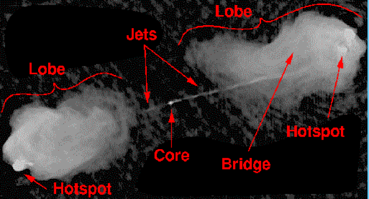
More than a decade after its commissioning, the VLA has been equipped with low-frequency receivers at 74 and 330 MHz. At these frequencies, the field of view is so wide that the sky can no longer be approximated by a 2-dimensional plane, and 3-dimensional Fourier transforms are necessary to produce meaningful images. Some examples are given at rsd-www.nrl.navy.mil/7214/weiler/4bandfarm.html.
6.4 Spectral Lines
There is a general scarcity of WWW resources on spectral line data. Integrated source parameters may be obtained from selected catalogues in the CDS archive, most conveniently consulted via vizier.u-strasbg.fr/cgi-bin/VizieR.
A list of transition frequencies from 701 MHz to 3.43 THz, with
references, has been published by [Lovas (1992)].
A compilation of links to “Worldwide Molecular Astrophysics Resources” is
offered at www.strw.leidenuniv.nl/~iau34/links.html.
It provides pointers to several useful mm-wave line databases.
The first of these links (dated June 1997) tells us that 114 molecules
have now been detected in space, containing between two and thirteen atoms
(HC11N).
One may search for known spectral lines by several parameters
(frequency range, type of molecule, line strength, etc.)
at the URLs spec.jpl.nasa.gov/ftp/pub/catalog/catform.html and
www.patnet.caltech.edu/~dmehring/find_lines.1.0.html.
6.4.1 Neutral Hydrogen (H I)
By the 1950s, radio astronomers had already mapped the profiles of the hyperfine transition of the ground state of the hydrogen atom at 1420 MHz (21.1 cm). From this they could infer, using the formulae by Lindblad & Oort for differential Galactic rotation, the spiral structure of the H I distribution in the northern ([Westerhout (1957)]), and later in both Galactic hemispheres (e.g. [Oort et al. (1958)]).
Later these surveys were extended beyond the Galactic plane to the whole sky, and apart from their importance for the distribution and kinematics of Galactic H I, they are also a necessary tool for X-ray astronomers to estimate the Galactic absorption (from the H I column density) in X-ray spectra of extragalactic objects, near 0.1 keV. Many of these H I surveys are now available in the CDS archive (e.g. catalogues VIII/7, 8, 9, 10, 11, and 47). Curiously, some of these “treasures”, e.g. the “Bell Laboratories H I Survey” by Stark et al. (1990; CDS/ADC # VIII/10) were never really published in an ordinary journal. Others, like VIII/47 ([Westerhout et al. (1982)]) are only now being prepared for integration into the CDS archive, 16 years after publication. The H I survey by [Strong et al. (1982)] was tracked down by the author, motivated by a poster displayed on the current winter school, and later found to exist in electronic form ! These authors used the Parkes 64-m dish to cover a Galactic plane region (=245∘through 12∘, 10∘), sampled every 0.5∘ in and 1∘ in with an angular resolution of 15′.
One of the largest very recent H I surveys is indeed available electronically, but not in a public archive. Between 1988 through 1993 the sky north of =30∘ was mapped with the Dwingeloo 25-m dish (HPBW=36′) on a grid of 30′ and with a velocity coverage of 850 km s-1. The data resulting from this Leiden-Dwingeloo H I Survey are not presently available on the Internet, but were published as an Atlas and a CD-ROM ([Hartmann & Burton (1997)]). On the CD, there are colour GIF files for all images in the Atlas, as well as animations running through the data cube in velocity space.
Integrated H I fluxes and line widths of galaxies may be obtained from LEDA, accessible via telnet to lmc.univ-lyon1.fr (login as leda), or enter via the WWW at www-obs.univ-lyon1.fr/leda. Currently LEDA offers H I fluxes for 12,400 of a total of 170,000 galaxies in LEDA.
H I observations of external galaxies (mainly the gas-rich late-type ones) are important for deriving their rotation curves and detailed kinematics (e.g. [Burton (1976)]). These (flat) rotation curves have led to further evidence for the so-called “dark matter haloes” in galaxies. Numerous detailed studies have been published over the past three decades, very little of which has been preserved in electronic form, except for compilations of rotation curve parameters (e.g. [Baiesi-Pillastrini et al. (1983)], [Persic & Salucci (1995)] and [Mathewson & Ford (1996)]). Also, [Martín (1998)] gives a compilation of bibliographic references to H I maps of 1439 galaxies published between 1953 and 1995, as well as parameters drawn from these maps.
A gallery of ATCA observations of H I in galaxies has been compiled
by B. Koribalski at www.atnf.csiro.au/~bkoribal/atca_obs.html.
6.4.2 Molecular and Recombination Lines, and Pulsars
Carbon monoxide (CO) emits one of the most abundant molecular lines in space, e.g. the 12CO(J=1-0) line at 115 GHz (=2.6 mm). These data allow one to infer the distribution of molecular hydrogen, e.g. in the plane of our Galaxy or throughout other galaxies. A composite survey of this line over the entire Milky Way ([Dame et al. (1987)]) at 8.7′ resolution is available as ADC/CDS catalogue # 8039 and at ADIL (§6.3.2). It was made with two 1.2-m dishes, one in New York City, the other in Chile, and provides 720 latitude-velocity maps as FITS files, one for each 30′ of Galactic longitude, and a velocity-integrated map. The Five College Radio Astronomy Observatory (FCRAO) has mapped 336 deg2 of the Galactic plane (102.5∘141.5∘, 3∘5.4∘) in the 12CO(1-0) line at 115 GHz with 45′′ resolution ([Heyer et al. (1998)]), available at ADIL (§6.3.2; imagelib.ncsa.uiuc.edu/document/97.MH.01), and at ADC. A survey of the 12CO(2-1) line at 230 GHz was made of the Galactic plane (20∘60∘ and 1∘) with 9′ resolution, using the 60-cm sub-mm telescope at Nobeyama ([Sakamoto et al. (1995)]). It is available at ADC and CDS (# J/ApJS/100/125/).
The “Catalog of CO Observations of Galaxies” ([Verter (1985)])
(ADC/CDS # 7064) is now largely outdated.
The “FCRAO Extragalactic CO survey” has measured 1412 positions in 300 galaxies
with the 14-m dish at FCRAO (HPBW=45′′, [Young et al. (1995)]) in
the 12CO(1-0) line. It is apparently not available on the WWW, although its
natural home appears to be the URL donald.phast.umass.edu/~fcrao/library/.
The “Swedish ESO Submillimetre Telescope” (SEST) and the 20-m Onsala dish
were used to search for CO in 168 galaxies ([Elfhag et al. (1996)]).
The Nobeyama 45-m single dish has surveyed 27 nearby spirals in the
12CO(1-0) line ([Nishiyama & Nakai (1998)]).
Other comprehensive molecular line surveys and lists of transition frequencies have been published (not in electronic form) in [Sutton et al. (1985)], [Turner (1989)], and [Schilke et al. (1997)].
Radio recombination lines occur through transitions of electrons between two energy states with very high quantum number . These lines are named after the atom, the destination quantum number and the difference in of the transition ( for =1, for =2, for =3, etc.). Examples are H 157 (transition from =158 to =157 in hydrogen) or He 109 (transition from =111 to =109 in helium). They are mainly used to map departures from thermal equilibrium, and the velocity structure in H II regions or in planetary nebulae. To my knowledge there is no WWW site offering data on recombination lines, but see www.hartrao.ac.za/spectra/SP_Hii.html for an introduction to the research done with this type of observation. See [Lilley & Palmer (1968)] and [Towle et al. (1996)] for tables of radio recombination lines.
A successful search for pulsars over the entire southern sky with the Parkes 64-m dish, the so-called 70-cm Pulsar Survey or “Parkes Southern Pulsar Survey” detected 298 pulsars, 101 of them previously unknown ([Lyne et al. (1998)]).
7 Finding Literature, Addresses, and Proposal Forms on WWW
7.1 Relevant Literature on the Internet
As in other branches of astronomy, much of the most recent publications can be found on the WWW. The LANL/SISSA electronic preprint server (xxx.lanl.gov) has been described in some detail in my tutorial. Radio astronomy topics are becoming increasingly popular on this server, although some of the most productive radio astronomy institutions have not yet discovered its efficiency and cost savings for the distribution of their preprints. Some institutions offer at least the titles of their preprints (if not full versions) on the WWW. Those preprints still circulated only on paper may be found in the STEP- and RAPsheets of the STScI and NRAO (sesame.stsci.edu/lib/stsci-preprint-db.html and libwww.aoc.nrao.edu/aoclib/rapsheet.html). Among the comprehensive collection of astronomy newsletters at sesame.stsci.edu/lib/NEWSLETTER.htm, there are several of interest to radio astronomers, depending on their area of research.
A few relevant proceedings volumes are also accessible on the WWW, e.g. the one on “Energy Transport in Radio Galaxies and Quasars” ([Hardee et al. (1996)]) discusses a wide variety of phenomena encountered in extragalactic radio sources, and papers from this volume are available as PostScript files from www.cv.nrao.edu/jetworks. Three other volumes ([Cohen & Kellermann (1995), Zensus et al. (1995), Zensus et al. (1998)]) bring together recent advances in high-resolution radio imaging of compact radio sources (see www.pnas.org/, www.cv.nrao.edu/vlbabook, and www.cv.nrao.edu/iau164/164book.html).
7.2 Finding Radio Astronomers around the World
Directories of astronomers in general have been described in section 7 of my tutorial for this winter school. Commission 40 (“Radio Astronomy”) of the IAU offers a list of its 860 members (sma-www.harvard.edu/IAU_Com40/IAU_scroll.html), and 660 of them appear with their email address.
7.3 Proposing Observations with Radio Telescopes
Like in most other parts of the electromagnetic spectrum,
proposals are accepted via email at most radio observatories.
Many of them offer their proposal forms on the WWW, like
e.g. for the various NRAO telescopes
at www.nrao.edu/proposals.html, for the ATNF telescopes
at www.atnf.csiro.au/observers/apply/form.html
(including Parkes and VLBI),
for MERLIN at www.jb.man.ac.uk/merlin/propsub/,
for the Arecibo dish at www.naic.edu/vscience/proposal/proposal.htm,
for the BIMA mm array at
www.astro.uiuc.edu/~bima/call_for_proposals.html,
or for the JCMT at www.jach.hawaii.edu/JCMT/pages/apply.html.
VLBI proposal forms for the EVN are available at
www.nfra.nl/jive/evn/proposals/prop.html, and for the VLBA see
the NRAO address above.
No web forms were found e.g. for the MRAO or IRAM telescopes,
nor for the WSRT.
Some institutions still require the proposals to be sent via regular
mail, e.g. the MPIfR Bonn
(www.mpifr-bonn.mpg.de/effelsberg/runkel/info_pke.html)
for proposing time at the Effelsberg 100-m dish.
It would be difficult here to give a comprehensive list of URLs
for the many radio
telescopes distributed over the globe.
8 The near and far Future of Radio Surveys and Telescopes
In this section I shall present some survey projects currently being carried out or planned, as well as some telescopes under construction or being designed. A good overview of current and planned radio astronomy facilities and recent research progress up to mid-1996 has been given in the latest Triennial Report of IAU Commision 40 (“Radio Astronomy”), at the URL sma2.harvard.edu/IAU_Com40/c40rpt/c40report.html. The next 3-year report is to become available in late 1999 at www.iau.org/div10.html. Many such projects have also been described in the proceedings volume by [Jackson & Davis (1997)].
8.1 Continuing or Planned Large-scale Surveys
On the island of Mauritius a 151 MHz survey is being performed with the “Mauritius Radiotelescope” (MRT; [Golap et al. (1995)]), and may be regarded as the southern continuation of the MRAO 6C survey (cf. Table 1). This T-shaped array of helical antennas provides an angular resolution of 44.6′ csc(z), where z is the zenith distance. The aim is to map the sky between declinations 10∘ and 70∘ to a flux limit of 200 mJy, including a map of the Galactic Plane and studies of pulsars. A catalogue of 105 sources can be expected after completion of the survey in summer 1998 (icarus.uom.ac.mu/mrt2.html).
After the completion of WENSS, the WSRT started in late 1997 the “WISH” survey at 350 MHz (www.nfra.nl/nfra/projects/index.htm). The aim is to survey the region of effective overlap with ESO’s “Very Large Telescope” (VLT; www.eso.org/projects/vlt/), which is limited by the WSRT horizon and by the elongation of the synthesised beam. In order to have a minimum hour angle coverage of 4 h, the area 30∘10∘, 10∘, or 5900 deg2, will be covered. With an expected noise limit of about 3 mJy (1-), and a source density of 20 per deg2, WISH should detect about 120,000 sources.
The DRAO Penticton aperture synthesis array is being used to survey the northern Galactic plane at 408 and 1420 MHz in the continuum, and at 1420 MHz in the H I line (www.drao.nrc.ca/web/survey.shtml). The area covered is 72∘ 140∘, 3∘5∘, and the angular resolutions are 1′ and 4′. First results of this survey can be viewed at www.ras.ucalgary.ca/pilot_project.html.
At MPIfR Bonn a 1.4 GHz Galactic plane survey (4∘20∘), using the Effelsberg 100-m dish in both total intensity and polarisation, is under way ([Uyanıker et al. (1998)]). Examples of how this survey will be combined with the NVSS, and with polarisation data from [Brouw & Spoelstra (1976)], have been shown by [Fürst et al. (1998)].
The first-epoch “Molonglo Galactic Plane Survey” (MGPS-1; [Green et al. (1998)]) at 843 MHz, was obtained with the old, 70′ field-of-view MOST and covers the region 245∘355∘, 1.5∘. The second-epoch Galactic plane survey (MGPS-2) is being made with the new, wide-field (2.7∘) system at 843 MHz, and will cover the region 240∘365∘, 10∘. With an angular resolution of 4343′′ csc and a noise level of 1–2 mJy/beam it is expected to yield over 80,000 sources above 5 mJy ([Green (1997)]). As a part of SUMSS (§3.7), it is well under way, and its survey images can be viewed at www.physics.usyd.edu.au/astrop/MGPS/. Catalogues of sources will be prepared at a later stage.
The Hartebeesthoek Radio Astronomy Group (HartRAO) in South Africa, after having finished the 2.3 GHz southern sky survey (§6.3.1), is planning to use its 26-m dish for an 8.4 GHz survey of the southern Galactic plane in total intensity and linear polarisation ([Jonas (1998)]) at 6′ resolution, and for deeper 2.3 GHz maps of interesting regions in the afore-mentioned 2.3 GHz survey.
8.2 Very Recent Medium-Deep Multi-Waveband Source Surveys
Between 1995 and 1997, the “AT-ESP” continuum survey was carried
out at 1.4 GHz with ATCA ([Prandoni et al. (1998)]).
This survey covers 27 deg2 near the South Galactic Pole
with a uniform sensitivity of 70 Jy (1 ).
About 3 000 radio sources have been detected, one third of them
being sub-mJy sources. Redshifts from the “ESO Slice Project”
(ESP) redshift survey for 3342 galaxies down to b 19.4
([Vettolani et al. (1998)],
boas5.bo.astro.it/~cappi/esokp.html)
will allow studies of the population of low-power radio galaxies
and of their 3-dimensional distribution.
The VLA has been used in C-configuration to carry out a sensitive 1.4 GHz
survey of 4.22 deg2 of the northern sky that have been surveyed also
in the Far Infra-Red with the ISO satellite, as part of
the “European Large Area ISO Survey” (ELAIS; [Ciliegi et al. (1998)],
www.ast.cam.ac.uk/~ciliegi/elais/).
The 5 flux limit of the survey ranges from
0.14 mJy (for 0.12 deg2) to 1.15 mJy (for the entire 4.22 deg2).
A careful comparison of the catalogue of 867 detected radio sources
with the FIRST and NVSS catalogues provided insights into the
reliability and resolution-dependent surface brightness effects
that affect interferometric radio surveys. Cross-identification with
IR and optical objects is in progress.
The “Phoenix Deep Survey” ([Hopkins et al. (1998)]) has used the ATCA
to map a 2∘ diameter region centred on (,)=
J 01h 14m 12.2s,45∘ 44′ 08′′.
A total of 1079 sources were detected above 0.2 mJy
(www.physics.usyd.edu.au/~ahopkins/cats).
Optical identifications were proposed for half of the sources,
and redshifts were measured for 135 of these.
A comparison with lower resolution 843 MHz MOST maps is in progress.
8.3 Extending the Frequency Range of the Radio Window
One of the very pioneers of radio astronomy, G. Reber, has been exploiting methods to observe cosmic radio emission at 2 MHz from the ground, even very recently. He quite successfully did so from two places in the world where the ionosphere appears to be exceptionally transparent (see [Reber (1994)] and [Reber (1995)]).
The lowest frequency observations regularly being made from the ground are done with the “Bruny Island Radio Spectrometer” ([Erickson (1997)]) on Bruny Island, south of Hobart (Tasmania). It is used for the study of solar bursts in the rarely observed frequency range from 3 to 20 MHz. Successful observations are made down to the minimum frequency that can propagate through the ionosphere. This frequency depends upon the zenith distance of the Sun and is usually between 4 and 8 MHz.
However, for many years radio astronomers have dreamt of extending the observing window to frequencies significantly below a few tens of MHz (where observations can be made more easily from the ground) to a few tens of kHz (just above the local plasma frequency of the interplanetary medium). Ionospheric absorption and refraction requires this to be done from space. The first radio astronomy at kHz frequencies, and the first radio astronomy from Space, was the “Radio Astronomy Explorer” (RAE; [Kaiser (1987)]), in the late 1960s and early 1970s. It consisted of a V-shaped antenna 450 m in extent, making it the largest man-made structure in space. It was equipped with radiometers for 25 kHz to 13.1 MHz. Although no discrete Galactic or extragalactic sources were detected, very crude all-sky maps were made, and solar system phenomena studied. Since then none of the various space projects proposed have been realised. Recent plans for developing low-frequency radio astronomy, both from the ground and from space, can be viewed at rsd-www.nrl.navy.mil/7214/weiler by following the links to Low Frequency Radio Astronomy (LFRA) and associated pages, but see also the ALFA project (§8.7). The proceedings volume by [Kassim & Weiler (1990)] is full of ideas on technical schemes for very low-frequency radio observatories, and on possible astrophysical insights from them.
Efforts to extend the radio window to very high frequencies have
been much more serious and successful in the past two decades, and
have led to a whole new branch of “mm-wave astronomy”.
The multi-feed technique (§2.1) has seen a trend
moving away from just having a single receiver in the focal plane,
towards having multiple receivers there, to help speed up the data collection
(as e.g. in the Parkes H I multibeam survey, §8.4).
By building big correlators, and taking
the cross-products between the different beams, the complex field
distribution in the focal plane of a dish may be mapped, and by
transforming that one can correct for pointing, dish deformation, etc.
Arrays of, say, 32 by 32 feeds are able to “image” the sky in real time
(see e.g. the SEQUOIA system at the FCRAO 14-m dish,
donald.phast.umass.edu/~fcrao/instrumentation/).
This is only possible at mm wavelengths, where the equipment is small enough
to fit into the focal plane. In perhaps three years such receivers should
exist at 100 GHz (3 mm).
As mentioned in §3.4 there is a lack of large-area surveys at frequencies above 5 GHz. As [Condon (1998)] has pointed out, such surveys are made difficult since the beam solid angle of a telescope scales as and system noise generally increases with frequency, so the time needed to survey a given area of sky rises very rapidly above 5 GHz. However, a 7-beam 15 GHz continuum receiver being built for the GBT (§8.6) could cover a 1-degree wide strip along the Galactic plane in one day, with an rms noise of 2 mJy. Repeating it several times would provide the first sensitive and systematic survey of variable and transient Galactic sources, such as radio stars, radio-emitting -ray sources, X-ray sources, etc.
More promising for the investigation of possible new source populations at these high frequencies (§3.4) may be the results from the new CMB satellites. One is the “Microwave Astronomy Probe” (MAP; map.gsfc.nasa.gov/html/web_site.html), expected to be launched by NASA in 2000. It will operate between 22 and 90 GHz with a 1.41.6 m diameter primary reflector, offering angular resolutions between 18′ and 54′. The other one is PLANCK (astro.estec.esa.es/SA-general/Projects/Planck/), to be launched by ESA in 2006 (possibly on the same bus as the “Far InfraRed and Submillimetre Telescope”, FIRST, not to be confused with the VLA FIRST radio survey). PLANCK will have a telescope of 1.5 m aperture, and it will be used with radiometers for low frequencies (30–100 GHz; =3–10 mm), and with bolometers for high frequencies (100–857 GHz; 0.3–3.0 mm), with angular resolutions of 10′ at 100 GHz. Both the MAP and PLANCK missions should detect a fair number of extragalactic sources at 100 GHz (=3 mm). In fact, [Tegmark & De Oliveira-Costa (1998)] expect PLANCK to detect 40,000 discrete sources at 857 GHz. A highly important by-product will be the compilation of a much denser grid of calibration sources at mm wavelengths. The vast majority of the currently known mm-wave calibrators are variable anyway.
8.4 Spectral Line and Pulsar Surveys
The Australia Telescope National Facility (ATNF) has constructed and commissioned a 21-cm multi-feed system with 13 receivers at the prime focus of the Parkes 64-m telescope ([Staveley-Smith (1997)]; wwwpks.atnf.csiro.au/people/multi/multi.html). The feeds are disposed to form beams with an angular resolution of 14′ and a distance of 28′ between neighbouring feeds. The on-line correlator measures flux density in all 13 channels and 2 polarisations simultaneously, with a spectral resolution of 16 km s-1 and a velocity range from 1200 km s-1 to 12,700 km s-1. The Parkes multi-beam facility commenced regular observing in 1997, and a report on its status is regularly updated at www.atnf.csiro.au/research/multibeam/multibeam.html. Several major H I surveys are planned, including an “all-sky” survey (20∘) with a limiting sensitivity (5, 600 s) of 20 mJy per channel. The Zone of Avoidance (ZOA, 5∘) will be covered with the same velocity range and twice the sensitivity. It will be sensitive to objects with H I mass between 106 and 1010 M⊙, depending on distance. This will be the first extensive “blind” survey of the 21-cm extragalactic sky. When scheduled, it is possible to watch the signal of all 13 beams almost in real time at wwwpks.atnf.csiro.au/people/multi/public_html/live/multibeam_live.html. An extension of this survey to the northern hemisphere (20∘) will be performed with the Jodrell-Bank 76-m Mark I antenna, but only 4 receivers will be used.
This Parkes multibeam system is also being used for a sensitive wide-band continuum search for pulsars at 1.4 GHz, initially limited to the zone 220∘20∘ within 5∘ from the Galactic plane. A first observing run in August 1997 suggested that 400 new pulsars may be found in this survey, which is expected to take 100 days of telescope time at Parkes, spread over two years (ATNF Newsletter 34, p. 8, 1998).
The “Westerbork observations of neutral Hydrogen in Irregular and SPiral
galaxies” (WHISP; www.astro.rug.nl/~whisp)
is a survey to obtain WSRT maps of the distribution and velocity
structure of H I in 500 to 1000 galaxies, increasing the number of
galaxies with well-studied H I observations by an order of magnitude.
By May 1998 about 280 galaxies had been observed, and the data had been
reduced for 160 of them.
H I profiles, velocity maps, and optical finding charts
are now available for 150 galaxies. Eventually the data cubes and
(global) parameters of all galaxies will also be made available.
The Dwingeloo 25-m dish is currently pursuing the “Dwingeloo Obscured Galaxy Survey” (DOGS; [Henning et al. (1998)]; www.nfra.nl/nfra/projects/dogs.htm) of the area 30∘220∘; 5.25∘. This had led to the discovery of the nearby galaxy Dwingeloo 1 in August 1994 ([Kraan-Korteweg et al. (1994)]). After a shallow survey in the velocity range 0–4000 km s-1 with a noise level of 175 mJy per channel, a second, deeper survey is being performed to a noise level of 40 mJy. The latter has so far discovered 40 galaxies in an area of 790 deg2 surveyed to date.
The first results of a dual-beam H I survey with the Arecibo 305-m dish have been reported in [Rosenberg & Schneider (1998)]. In a 400 deg2 area of sky 450 galaxies were detected, several of them barely visible on the Palomar Sky Survey.
Since 1990, the Nagoya University has been executing a 13CO(1-0) survey at 110 GHz of the Galactic plane, with a 4-m mm-wave telescope. Since 1996, this telescope is operating at La Silla (Chile) to complete the southern Galactic plane ([Fukui & Yonekura (1998)]). The BIMA mm-array is currently being used to survey 44 nearby spiral galaxies in the 12CO(1-0) line at 6′′–9′′ resolution ([Helfer et al. (1998)]).
8.5 CMB and Sunyaev-Zeldovich Effect
The cosmic microwave background (CMB) is a blackbody radiation of 2.73 K and has its maximum near 150 GHz (2 mm). Measurements of its angular distribution on the sky are highly important to constrain cosmological models and structure formation in the early Universe, thus the mapping of anisotropies of the CMB has become one of the most important tools in cosmology. For a summary of current CMB anisotropy experiments, see [Wilkinson (1998)] and [Bennett et al. (1997)]; the latter even lists the relevant URLs (cf. also brown.nord.nw.ru). As an example, the Cambridge “Cosmic Anisotropy Telescope” (CAT; [Robson et al. (1993)], www.mrao.cam.ac.uk/telescopes/cat/) has started to map such anisotropies, and it is the prototype for the future, more sensitive “Very Small Array” (VSA; §8.6.2).
The “Sunyaev-Zeldovich” (SZ) effect is the change of brightness temperature of the CMB towards regions of “hot” (T 107 K) thermal plasma, typically in the cores of rich, X-ray emitting clusters of galaxies. The effect is due to the scattering of microwave photons by fast electrons, and results in a diminution of below 200 GHz, and in an excess of above that frequency. See [Birkinshaw (1998)] for a comprehensive review of past observations and the potential of these for cosmology. See [Liang & Birkinshaw (1998)] for the status and future plans for observing the Sunyaev-Zeldovich effect.
8.6 Radio Telescopes: Planned, under Construction or being Upgraded
8.6.1 Low and Intermediate Frequencies
The Arecibo observatory has emerged in early 1998 from a 2-year upgrading phase (www.naic.edu/techinfo/teltech/upgrade/upgrade.htm). Thanks to a new Gregorian reflector, the telescope has a significantly increased sensitivity.
The National Centre for Radio Astrophysics (NCRA) of the Tata Institute for Fundamental Research (TIFR, India) is nearing the completion of the “Giant Metrewave Radio Telescope” (GMRT) at a site about 80 km north of Pune, India (www.ncra.tifr.res.in). With 30 fully steerable dishes of 45 m diameter, spread over distances of up to 25 km, it is the world’s most powerful radio telescope operating in the frequency range 50–1500 MHz with angular resolutions between 50′′ and 1.6′′. In June 1998, all 30 dishes were controllable from the central electronics building. Installation of the remaining feeds and front ends is expected in summer 1998. The digital 30-antenna correlator, combining signals from all the antennas to produce the complex visibilities over 435 baselines and 256 frequency channels, is being assembled, and it will be installed at the GMRT site also in summer 1998. The entire GMRT array should be producing astronomical images before the end of 1998.
The NRAO “Green Bank Telescope” (GBT; www.gb.nrao.edu/GBT/GBT.html) is to replace the former 300-ft telescope which collapsed in 1988 from metal fatigue. The GBT is a 100-m diameter single dish with an unblocked aperture, to work at frequencies from 300 MHz to 100 GHz, with almost continuous frequency coverage. It is finishing its construction phase, and is expected to be operational in 2000 ([Vanden Bout (1998)]).
The VLA has been operating for 20 years now, and a plan for an upgrade has been discussed for several years. Some, not very recent, information may be found at the URL www.nrao.edu/vla/html/Upgrade/Upgrade_home.shtml. Among other things, larger subreflectors, more antennas, an extension of the A-array, a super-compact E-array for mosaics of large fields, and continuous frequency coverage between 1 and 50 GHz are considered.
An overview of current VLBI technology and outlooks for the future of VLBI have been given in the proceedings volume by [Sasao et al. (1994)].
For several years the need for and the design of a radio telescope with a collecting area of one square kilometre have been discussed. The project is known under different names : the “Square Kilometre Array Interferometer” (SKAI; www.nfra.nl/skai/; [Brown (1996)]); the “Square Kilometre Array” (SKA; www.drao.nrc.ca/web/ska/ska.html), and the “1-km teleskope” (1kT; www.atnf.csiro.au/1kT). A Chinese version under the name “Kilometer-square Area Radio Synthesis Telescope” (KARST; www.bao.ac.cn/bao/LT) was presented by [Peng & Nan (1998)], and contemplates the usage of spherical (Arecibo-type) natural depressions, frequently found in southwest China, by the placing of 30 passive spherical reflectors, of 300 m diameter, in each of them. A frequency coverage of 0.2–2 GHz is aimed at for such an array of reflectors.
A new design for a large radio telescope, based on several almost flat primary reflectors, has been recently proposed ([Legg (1998)]). The reflectors are adjustable in shape, and are of very long focal length. The receiver is carried by a powered, helium-filled balloon. Positional errors of the balloon are corrected either by moving the receiver feed point electronically, or by adjusting the primary reflector so as to move its focal point to follow the balloon. The telescope has the wide sky coverage needed for synthesis observations and an estimated optimum diameter of 100–300 m. It would operate from decimetre to cm-wavelengths, or, with smaller panels, mm-wavelengths.
8.6.2 Where the Action is: Millimetre Telescopes and Arrays
The “Smithsonian Submillimeter Wavelength Array” (SMA; sma2.harvard.edu/) on Mauna Kea (Hawaii) consists of eight telescopes of 6 m aperture, six of these provided by the Smithsonian Astrophysical Observatory (SAO) and two by the Astronomica Sinica Institute of Astronomy and Astrophysics (ASIAA, Taiwan). Eight receivers will cover all bands from 180 to 900 GHz (=1.7–0.33 mm). To achieve an optimised coverage of the uv plane, the antennas will be placed along the sides of Reuleaux triangles, nested in such a way that they share one side, and allow both compact and wide configurations. Baselines will range from 9 to 460 m, with angular resolutions as fine as 0.1′′. The correlator-spectrometer with 92,160 channels will provide 0.8 MHz resolution for a bandwidth of 2 GHz in each of two bands. One of the SMA telescopes has had “first light” in spring 1998, and the full SMA is expected to be ready for observations in late 1999.
Since April 1998, the ATNF is being upgraded to become the first southern hemisphere mm-wave synthesis telescope (cf. ATNF Newsletter 35, Apr 1998). The project envisages the ATNF to be equipped with receivers for 12 and 3 mm ([Norris (1998)]).
The “Millimeter Array” (MMA; www.mma.nrao.edu/) is a project by NRAO to build an array of 40 dishes of 8–10 m diameter to operate as an aperture synthesis array at frequencies between 30 and 850 GHz (0.35–10 mm). Array configurations will range from about 80 m to 10 km. It will most probably be placed in the Atacama desert in northern Chile at an altitude near 5000 m, a site rivalling the South Pole in its atmospheric transparency ([Vanden Bout (1998)]).
The “Large Southern Array” project (LSA) is coordinated by ESO, IRAM, NFRA and Onsala Space Observatory (OSO), and it anticipates the building of a large millimetre array with a collecting area of up to 10,000 m2, or roughly 10 times the collecting area of today’s largest millimetre array in the world, the IRAM interferometer at the Plateau de Bure with five 15-m diameter telescopes. With baselines foreseen to extend to 10 km, the angular resolution provided by the new instrument will be that of a diffraction-limited 4-m optical telescope. Current plans are to provide the collecting area equivalent to 50–100 dishes of between 11 and 16 m diameter, located on a plain above 3000 m altitude. Currently only site testing data are available on the WWW (puppis.ls.eso.org/lsa/lsahome.html).
A similar project in Japan, the “Large Millimeter and Submillimeter Array” (LMSA; www.nro.nao.ac.jp/LMSA/lmsa.html) anticipates the building of a mm array of 50 antennas of 10 m diameter each, with a collecting area of 3,900 m2, to operate at frequencies between 80 and 800 GHz.
The MMA, LSA and LMSA projects will be so ambitious that negotiations to join the LMSA and MMA projects, and perhaps all three of them, are under way. The name “Atacama Array” has been coined for such a virtual instrument (see NRAO Newsletter # 73, p. 1, Oct. 1997). The MMA will also pose challenging problems for data archiving, and in fact will rely on a new data storage medium to enable archiving to be feasible (cf. www.mma.nrao.edu/memos/html-memos/abstracts/abs164.html).
A comparison of current and future mm arrays is given in Table 3.
| Array | Completion | Wavelength | Sensitivity b | max baseline |
|---|---|---|---|---|
| Date | Range (mm) | at 3mm (Jy) | (km) | |
| Nobeyama (6 10 m) | 1986 | 3.0, 2.0 | 1.7 | 0.36 |
| IRAM (5 15 m) | 1988 | 3.0, 1.5 | 0.3–0.8 | 0.4 |
| OVRO (6 10.4 m) | 1990 ? | 3.0, 1.3 | 0.5 | 0.3 |
| BIMA (9 6 m) | 1996 | 3.0 (1.3) | 0.7 | 1.4 |
| SMA CfA (8 6 m) | 1999 ? | 1.7–0.33 | - | 0.46 |
| ATCA (5 22 m) | 2002 ? | 12.0, 3.0 | 0.5 ? | 3.0 (6.0 ?) |
| MMA USA (40 10 m?) | 2010 ? | 10.0–0.35 | 0.04 ? | 10.0 |
| LSA Europe (50 ? 16 m?) | 2010 ? | 3.0, 1.3,… | 0.02 ? | 10.0 |
| LMSA Japan (50 10 m) | 2010 ? | 3.5–0.35 | 0.03 ? | 10.0 |
a) adapted from [Norris (1998)], but see also [Stark et al. (1998)] for mm-wave single dishes
b) rms continuum sensitivity at 100 GHz to a point source observed for 8 hours
The “Large Millimeter Telescope” (LMT) is a 50-m antenna to be built on the slopes of the highest mountain in Mexico in the Sierra Negra, 200 km east of Mexico City, at an elevation of 4500 m. It will operate at wavelengths between 8.5 and 35 GHz (=0.85–3.4 mm) achieving angular resolutions between 5′′ and 20′′ (see lmtsun.phast.umass.edu/).
There are plans for a 10-m sub-mm telescope at the South Pole
([Stark et al. (1998)]; cfa-www.harvard.edu/~aas/tenmeter/tenmeter.html).
The South Pole has been identified as the best site for sub-mm wave astronomy
from the ground. The 10-m telescope will be suitable for “large-scale” (1 deg2)
mapping of line and continuum from sub-mm sources at mJy flux levels, at
spatial resolutions from 4′′ to 60′′, and it will make
arcminute scale CMB measurements.
The “Very Small Array” (VSA; www.jb.man.ac.uk/~sjm/cmb_vsa.htm;
astro-ph/9804175), currently in the design phase, consists
of a number of receivers with steerable horn antennas, forming an aperture
synthesis array to work at frequencies around 30 GHz (=10 mm).
It will be placed at the Teide Observatory on Tenerife (Spain)
around the year 2000. The VSA will provide images of structures
in the CMB, on angular scales from 10′ to 2∘. Such
structures may be primordial, or due to the SZ effect (§8.5)
of clusters of galaxies beyond the limit of current optical sky surveys.
The “Degree Angular Scale Interferometer” (DASI; astro.uchicago.edu/dasi)
is designed to measure anisotropies in the CMB, and consists of 13 closely
packed 20-cm diameter corrugated horns, using cooled High Electron Mobility
Transistor (HEMT) amplifiers running
between 26 and 36 GHz. It will operate at the South Pole by late 1999.
A sister instrument, the “Cosmic microwave Background Interferometer”
(CBI; astro.caltech.edu/~tjp/CBI/) will be located at high
altitude in northern Chile, and it will probe the CMB on smaller angular scales.
8.7 Space Projects
Radioastron ([Kardashev (1997)]; www.asc.rssi.ru/radioastron/) is an international space VLBI project led by the “Astro Space Center” of the Lebedev Physical Institute in Moscow, Russia. Its key element is an orbital radio telescope that consists of a deployable 10-m reflector made of carbon fiber petals. It will have an overall rms surface accuracy of 0.5 mm, and operate at frequencies of 0.33, 1.66, 4.83 and 22.2 GHz. It is planned to be launched in 2000–2002 on a Proton rocket, into a highly elliptical Earth orbit with an apogee of over 80 000 km.
The “Swedish-French-Canadian-Finnish Sub-mm Satellite” (ODIN) will carry a 1.1-m antenna to work in some of the unexplored bands of the electromagnetic spectrum, e.g. around 118, 490 and 560 GHz. The main objective is to perform detailed studies of the physics and the chemistry of the interstellar medium by observing emission from key species. Among the objects to be studied are comets, planets, giant molecular clouds and nearby dark clouds, protostars, circumstellar envelopes, and star forming regions in nearby galaxies (see kurp-www.hut.fi/spectroscopy/space-projects.shtml).
A new space VLBI project, the “Advanced Radio Interferometry between Space and Earth” (ARISE) has recently been proposed by [Ulvestad & Linfield (1998)]. It consists in a 25-m antenna in an elliptical Earth orbit between altitudes of 5,000 and 40,000 km, operating at frequencies from 5 to 90 GHz. The estimated launch date is the year 2008.
A space mission called “Astronomical Low-Frequency Array” (ALFA) has been proposed to map the entire sky between 30 kHz and 10 MHz. The project is in the development phase (sgra.jpl.nasa.gov/html_dj/ALFA.html) and no funding exists as yet.
The far side of the Moon has been envisaged for a long time as an ideal site for radio astronomy, due to the absence of man-made interference. Speculations on various kinds of radio observatories on the Moon can be found in the proceedings volumes by [Burns & Mendell (1988)], [Burns et al. (1989)], and [Kassim & Weiler (1990)]. Since then, the subject has been “dead” as there has been no sign of interest by the major space agencies in returning to the Moon within the foreseeable future.
8.8 Nomenclature and Databases
More and more astronomers rely on databases like NED, SIMBAD & LEDA, assuming they are complete and up-to-date. However, researchers should make life easier for the managers of these databases, not only by providing their results and data tables directly to them, but also by making correct references to astronomical objects in their publications. According to IAU recommendations for the designation of celestial objects outside the solar system (cdsweb.u-strasbg.fr/iau-spec.html), existing names should neither be changed nor truncated in their number of digits. Acronyms for newly detected sources, or for large surveys, should be selected carefully so as to avoid clashes with existing acronyms. The best way to guarantee this is to register a new acronym with the IAU at vizier.u-strasbg.fr/cgi-bin/DicForm. For example, in D. Levine’s lectures for this winter school the meaning of FIRST is very different from that in the present paper (cf. §8.3). Together with the Task Group on Designations of Commission 5 of the IAU, the author is currently involved in a project to allow authors to check their preprints for consistency with current recommendations. This should not be seen just as a further obstacle for authors, but as an offer to detect possible non-conforming designations which are likely to lead to confusion when it comes to the ingestion of these data into public databases.
9 Summary of Practicals
Two afternoons of three to four hours were set aside for exercises using the WWW facilities listed in these lectures. In the first practical, the students were offered the names of five very extended ( 20′) radio galaxies from the 3C catalogue, and asked to find out the positions of one or more of them from NED or SIMBAD, to obtain an optical finding chart from one of the various DSS servers, and to plot these with sky coordinates along the margins. The next task was to extract a 1.4 GHz radio image from the NVSS survey, and a list of sources from the NVSS catalogue of the same region. A comparison of the two gave an idea of how well (or less well) the catalogued sources (or components) represent the real complex structures of these sources. The students were also asked to look at higher-resolution images of these sources in the “Atlas of DRAGNs”. A further exercise was to find out where the many names under which these sources were known in NED or SIMBAD come from, by looking up the acronyms in the On-line Dictionary of Nomenclature. The optical object catalogues like APM, APS and COSMOS were then queried for the same regions of sky, which allowed the object classification as star or galaxy to be checked by comparison with the optical charts from the DSS server. Eventually, radio images from the FIRST survey were extracted in order to see to what extent the large-scale structure of the radio galaxies could still be recognised.
In the second practical, the students were given a chance to discover a new, optically bright radio-loud quasar, a radio galaxy, a starburst galaxy, or even a radio star! Each of the roughly two dozen participating students was assigned a region of sky of the size of a Palomar plate (6.5∘6.5∘) in the zone 08RA16h, 22∘42∘ (the region covered by the FIRST 1.4 GHz survey at that time). Each student was asked to extract all bright objects (10 magB17 mag) from the USNO A1.0 catalogue (cf. § 3 of my tutorial) in the region assigned to them. This was done by remote interrogation of the USNO site, using the command findpmm from the CDS client software, which had been installed for the school on the computers at the IAC. The resulting object list (typically 3,000–10,000 objects per student, depending on the Galactic latitude of the assigned field) was reformatted so as to serve as input for interrogation of the NVSS source catalogue, which I had installed at the IAC for the winter school. It had 1.67 million sources in Nov. 1997. The FORTRAN program NVSSlist, publicly available from NRAO, was used to search a circle of radius 10′′ around each optical object in the NVSS catalogue, limited to 1.4 GHz fluxes greater than 10 mJy so as to assure the positional accuracy of the radio sources. The students were asked to estimate the chance coincidence rate, and they found that between 0.5 and 2 matches were to be expected by chance. Actually each student had between three and 18 “hits” and was asked to concentrate on the optically or radio-brightest objects to find out whether the identification was correct, whether it was new, and what was known previously about the object. For promising candidates, a search in the FIRST 1.4 GHz image database was suggested, as well as an extraction of a DSS image. Some students even managed a radio-optical overlay, and one of them found that the overlay facility in SkyView had a bug when the pixel sizes of the overlaid images (like e.g. NVSS and DSS) was not identical. This was later reported to, acknowledged and fixed by the SkyView team. Unfortunately the FIRST image server went “out of service” right during the practical.
With the 23 participating students, a sky area of 800 deg2 had been covered, and a cross-identification of altogether 80,000 optical objects with 12,500 radio sources was accomplished. Fifteen students sent me their results, of which only the most spectacular will be mentioned here. The 13.9 mag IRAS galaxy NGC 3987 almost filled the 33′ DSS image (which the students were asked to extract) and gave a splendid appearance with its edge-on orientation and strong dust lane. It was found to coincide with a 58 mJy NVSS source extended along the disk of the galaxy, while FIRST clearly shows a strong compact source (AGN?) and weak radio emission along the disk. A subsequent search in NED turned up a few other detailed radio studies ([Burns et al. (1987)], [Condon & Broderick (1986b)], and [Jaffe et al. (1986)]). Comparison of the 609 MHz flux from the latter reference shows that the compact central source has an inverted spectrum (rising with frequency), apparently not noticed before in literature. Another student came across UGC 5146 (Arp 129), an interacting pair. While the FIRST image server was unavailable, the FIRST catalogue showed it to be a very complex source, aligned along the connecting line between the pair, and very extended. A third student “rediscovered” the well-known Seyfert galaxy NGC 4151 with its 600 mJy nuclear point source. At first sight no bright radio star had been discovered, not surprising given the more thorough searches for radio stars now available (§3.6).
10 Conclusions
This was a most unusual and rewarding winter school, and exhausting for lecturers, students and organisers. The organisers are to be congratulated for the excellent planning and running of the school, and the IAC for its vision and courage to choose such a topic, which, at least when it comes to requests for funding, is often claimed to lack merit, and to be regarded as not scientific. The school has clearly proven that scientific expertise is a prerequisite for constructing and maintaining data archives, databases, and WWW interfaces, so as to make them user-friendly and reliable at the same time. Too much effort is often spent on fancy user interfaces, rather than on the content or its adequate documentation in an archive or database.
I have tried to show that more concerted effort is necessary to avoid duplication of similar WWW facilities, and the deterioration of WWW pages with outdated information. Much effort is being spent by individuals, without an institutional support or obligation, in providing useful WWW pages. The advantage is that these are often highly motivated and qualified researchers, but also with the disadvantage that the service will likely be discontinued with personal changes.
I also hope that my lectures will stimulate the use of archives both for advanced research as well as for thesis projects. Nevertheless, the warnings and pointers to possible pitfalls I have tried to strew about my lectures cannot replace a sound observational experience during the first years of research.
Clearly, the educational possibilities of the Internet have not been fully exploited. In fact, this winter school, gathering 50 students in one place and putting them in front of 25 computer terminals, to go and try what they had been taught during the lectures, may have been an interim between a classical school without hands-on exercises and a fully distributed and interactive one, where students would follow lectures over the WWW and perform exercises at home.
Acknowledgements.
I am grateful to the organisers for inviting me to give these lectures, and for their financial support. The persistence and excitement of the students during the practicals was truly impressive. These practicals would have been impossible without the excellent computing facilities prepared for the school by R. Kroll and his team of the “Centro de Calculo” of the IAC. I would like to thank the many people who provided useful information, enriching and completing these lecture notes : D. Banhatti, E. Brinks, S. Britzen, J. Burns, J.J. Condon, W.R. Cotton, G. Dulk, W. Erickson, L. Feretti, G. Giovannini, Gopal Krishna, L. Gurvits, S.E.G. Hales, R.W. Hunstead, S. J. Katajainen, K. Kingham, N. Loiseau, V. Migenes, R. Norris, E. Raimond, W. Sherwood, S. A. Trushkin, K. Weiler, and Rick L. White. Thanks also go to all authors of useful WWW pages with compilations of links which I came across while surfing the WWW for this contribution. This paper has made use of NASA’s Astrophysics Data System Abstract Service. A. Koekemoer provided help to print Figure 1 successfully, E. Tago kindly helped to produce Figure 6, and special thanks also go to A.C. Davenhall, A. Fletcher, S. Kurtz, and O.B. Slee for their careful reading of the manuscript at the very last moment. All of them strengthened my belief that most of the information given here must have been correct at least at some point in time. Last, but not least, the Editors of this volume are thanked for their eternal patience with the delivery of this report.References
- Abell et al. (1989) Abell, G. O., Corwin, H. G. Jr, & Olowin, R. P. 1989, ApJS 70, 1–138
- Acker et al. (1991) Acker, A., Stenholm, B., & Véron, P. 1991, A&AS 87, 499
- Acker & Stenholm (1990) Acker, A., & Stenholm, B. 1990, A&AS 86, 219–225
- Altenhoff et al. (1979) Altenhoff, W. J., Downes, D., Pauls, T., & Schraml, J. 1979, A&AS 35, 23–54
- Altschuler (1986) Altschuler, D. R. 1986, A&AS 65, 267–283
- Amirkhanyan et al. (1989) Amirkhanyan, V. R., Gorshkov, A. G., Larionov, M. G., Kapustkin, A. A., Konnikova, V. K., Lazutkin, A. N., Nikanorov, A. S., Sidorenkov, V. N., & Ugol’kova, L. S. 1989, The Zelenchuk Survey of Radio Sources between Declinations 0∘and 14∘, MIR Publ., Moscow, ISBN 5-211-01151-1
- Andernach (1989) Andernach, H. 1989, Bull. Inf. CDS 37, 139–141
- Andernach (1990) Andernach, H. 1990, Bull. Inf. CDS 38, 69–94
- Andernach (1992) Andernach H. 1992, in Astronomy from Large Data Bases – II, eds. A. Heck & F. Murtagh, ESO Conf. & Workshop Proceedings, 43, 185–190, ESO, Garching
- Andernach et al. (1992) Andernach, H., Feretti, L., Giovannini, G., Klein, U., Rossetti, E., & Schnaubelt, J. 1992, A&AS 93, 331–357
- Baade & Minkowski (1954) Baade, W., & Minkowski, R. 1954, ApJ 119, 206–214
- Baars et al. (1977) Baars, J. W. M., Genzel, R., Pauliny-Toth, I. I. K., & Witzel, A. 1977, A&A 61, 99–106
- Baiesi-Pillastrini et al. (1983) Baiesi-Pillastrini, G. C., Palumbo, G. G. C., & Vettolani, G. 1983, A&AS 53, 373–381
- Baldwin et al. (1985) Baldwin, J. E., Boysen, R. C., Hales, S. E. G., Jennings, J. E., Waggett, P. C., Warner, P. J., & Wilson, D. M. A. 1985, MNRAS 217, 717–730, microfiche
- Baleisis et al. (1998) Baleisis, A., Lahav, O., Loan, A. J., & Wall, J. V. 1998, MNRAS 297, 545–558
- Becker et al. (1991) Becker, R. H., White, R. L., & Edwards, A. L. 1991, ApJS 75, 1–229
- Becker et al. (1994) Becker, R. H., White, R. L., Helfand, D. J., & Zoonematkermani, S. 1994, ApJS 91, 347–387
- Bennett et al. (1986) Bennett, C. L., Lawrence, C. R., Burke, B. F., Hewitt, J. N., & Mahoney, J. 1986, ApJS 61, 1–104
- Bennett et al. (1997) Bennett, C. L., Turner, M. S., & White M. 1997, Physics Today, 50, 32–38
- Birkinshaw (1998) Birkinshaw, M. 1998, Phys. Rep., in press; www.star.bris.ac.uk/mb1/Export.html
- Bischof & Becker (1997) Bischof, O. B., & Becker, R. H. 1997, AJ 113, 2000–2005
- Boller et al. (1998) Boller, T., Bertoldi, F., Dennefeld, M., & Voges, W. 1998, A&AS 129, 87–145
- Bolton et al. (1949) Bolton, J. G., Stanley, G., & Slee, O. B. 1949, Nature, 164, 101
- Bolton et al. (1964) Bolton, J. G., Gardner, F. F., & Mackey, M. B. 1964, Aust. J. Phys. 17, 340
- Bozyan (1992) Bozyan, E. P. 1992, ApJS 82, 1–92
- Braude et al. (1979) Braude, S. Ia., Megn, A. V., Sokolov, K. P., Tkachenko, A. P., & Sharykin, N. K. 1979, Ap&SS 64, 73–126
- Braude et al. (1995) Braude, S. Y., Sokolov, K. P., Sharykin, N. K., & Zakharenko, S. M. 1995, Ap&SS 226, 245–271
- Bremer et al. (1998) Bremer, M., Jackson, N., & Pérez-Fournon, I. (eds.) 1998, Observational Cosmology with the New Radio Surveys, Kluwer Acad. Publ., ASSL vol. 226
- Brinkmann & Siebert (1994) Brinkmann, W., & Siebert, J. 1994, A&A 285, 812–818
- Brinks & Shane (1984) Brinks, E., & Shane, W. W. 1984, A&AS 55, 179–251
- Broten et al. (1988) Broten, N. W., MacLeod, J. M., & Vallée J.P. 1988, Ap&SS 141, 303–331
- Brouw & Spoelstra (1976) Brouw, W. N., & Spoelstra, T. A. Th. 1976, A&AS 26, 129–144
- Brown (1996) Brown, R. L. 1996, in The Westerbork Observatory, Continuing Adventure in Radio Astronomy, Kluwer Acad. Publ., Dordrecht, p. 167–183
- Burn (1966) Burn, B. J. 1966, MNRAS 133, 67–83
- Burns et al. (1983) Burns, J. O., Feigelson, E. D., & Schreier, E. J. 1983, ApJ 273, 128–153
- Burns et al. (1987) Burns, J. O., Hanisch, R. J., White, R. A., Nelson, E. R., Morrisette, K. A., & Ward, M. J. 1987, AJ 94, 587–617
- Burns & Mendell (1988) Burns, J. O., & Mendell, W. W. (eds.) 1988, Future Astronomical Observatories on the Moon, NASA Conf. Publ. 2489, Proc. of Workshop held in Houston, TX, USA, Jan. 1986
- Burns et al. (1989) Burns, J. O., Duric, N., Johnson, S., & Taylor, G. J. (eds.) 1989, A Lunar Far-Side Very Low Frequency Array, NASA Conf. Publ. 3039, Proc. of Workshop held in Albuquerque, NM, USA, Feb. 1988
- Bursov et al. (1997) Bursov, N. N., Lipovka, N. M., Soboleva, N. S., Temirova, A. V., Gol’neva, N. E., Parijskaya, E. Yu., & Savastenya, A. V. 1997, Bull. SAO 42, 5
- Burton (1976) Burton, W. B. 1976, ARA&A 14, 275–306
- Bystedt et al. (1984) Bystedt, J. E. V., Brinks, E., de Bruyn, A.G., Israel, F. P., Schwering, P. B. W., Shane, W. W., & Walterbos, R. A. M. 1984, A&AS 56, 245–280
- Christiansen & Högbom (1985) Christiansen, W. N. & Högbom, J. A. 1985, Radio Telescopes, 2nd ed., Cambridge University Press, Cambridge, UK
- Ciliegi et al. (1998) Ciliegi, P., McMahon, R. G., Miley, G., Gruppioni, C., Rowan-Robinson, M., Cesarsky, C., Danese, L., Franceschini, A., Genzel, R., Lawrence, A., Lemke, D., Oliver, S., Puget, J.-L., Rocca-Volmerange, B. 1998, subm. to MNRAS, astro-ph/9805353
- Cioffi & Jones (1980) Cioffi, D. F., & Jones, T. W. 1980, AJ 85, 368–375
- Clarke et al. (1976) Clarke, M. E., Little, A. G., & Mills, B. Y. 1976, Aust. J. Phys. Ap. Suppl. 40, 1–71
- Clarke et al. (1980) Clarke, J. N., Kronberg, P. P., & Simard-Normandin, M. 1980, MNRAS 190, 205–215
- Cohen & Kellermann (1995) Cohen, M. H., & Kellermann, K. I. 1995, Quasars and Active Galactic Nuclei : High Resolution Radio Imaging, Proc. Natl. Acad. Sci., USA, 92, 11339–11450
- Colla et al. (1970) Colla, G., Fanti, C., Fanti, R., Ficarra, A., Formiggini, L., Gandolfi, E., Grueff, G., Lari, C., Padrielli, L., Roffi, G., Tomasi, P., & Vigotti, M. 1970, A&AS 1, 281–317
- Colla et al. (1972) Colla, G., Fanti, C., Fanti, R., Ficarra, A., Formiggini, L., Gandolfi, E., Lari, C., Marano, B., Padrielli, L., & Tomasi, P. 1972, A&AS 7, 1–34
- Colla et al. (1973) Colla, G., Fanti, C., Fanti, R., Ficarra, A., Formiggini, L., Gandolfi, E., Gioia, I., Lari, C., Marano, B., Padrielli, L., & Tomasi, P. 1973, A&AS 11, 291–325
- Combi et al. (1998) Combi, J. A., Romero, G. E., & Arnal, E. M. 1998, A&A 333, 298–304
- Condon (1974) Condon, J. J. 1974, ApJ 188, 279–286
- Condon & Broderick (1986a) Condon, J. J., & Broderick, J. J. 1986a, AJ 91, 1051–1057
- Condon & Broderick (1986b) Condon, J. J., & Broderick, J. J. 1986b, AJ 92, 94–102
- Condon et al. (1989) Condon, J. J., Broderick, J. J., & Seielstad, G. A. 1989, AJ 97, 1064–1073
- Condon & Lockman (1990) Condon, J. J., & Lockman, F. J. 1990, Large-Scale Surveys of the Sky, Proc. NRAO Green-Bank Workshop No. 20, held Sept. 1987, publ. by NRAO, Charlottesville, WV, USA
- Condon et al. (1991) Condon, J. J., Broderick, J. J., & Seielstad, G. A. 1991, AJ 102, 2041–2046
- Condon et al. (1993) Condon, J. J., Griffith, M. R., & Wright, A. E. 1993, AJ 106, 1095–1100
- Condon et al. (1994) Condon, J. J., Broderick, J. J., Seielstad, G. A., Douglas, K., & Gregory, P. C. 1994, AJ 107, 1829–1833
- Condon et al. (1995) Condon, J. J., Anderson, E., & Broderick, J. J. 1995, AJ 109, 2318–2354
- Condon (1997) Condon, J. J. 1997, PASP 109, 166–172
- Condon et al. (1997) Condon, J. J., Kaplan, D. L., & Yin, Q. F. 1997, BAAS 29, 1231
- Condon (1998) Condon, J. J. 1998, IAU Symp. 179, 19–25, eds. B.J. McLean et al., Kluwer Acad. Publ., Dordrecht
-
Condon et al. (1998)
Condon, J. J., Cotton, W. D., Greisen, E. W., Yin, Q. F.,
Perley, R. A., Taylor, G. B., & Broderick, J. J. 1998,
AJ 115, 1693–1716;
www.cv.nrao.edu/~jcondon/nvss.html - Condon & Kaplan (1998) Condon, J. J., & Kaplan, D. L. 1998, ApJS, in press
- Cooray et al. (1998) Cooray, A. R., Grego, L., Holzapfel, W. L., Joy, M., & Carlstrom, J. E. 1998, AJ 115, 1388–1399
- Cornwell (1988) Cornwell, T. J. 1988, A&A 202, 316–321
- Cornwell (1989) Cornwell, T. 1989, in Synthesis Imaging in Radio Astronomy, eds. Perley, R. A., Schwab, F. R. & Bridle, A. H., ASP Conf. Ser. 6, ASP, San Francisco, p. 277–286
- Cornwell & Perley (1991) Cornwell, T. J. & Perley, R. A. (eds.) 1991, Radio Interferometry: Theory, Techniques, and Applications, ASP Conf. Ser. 19, ASP, San Francisco
- CRAF Handbook for Radio Astronomy (1997) CRAF Handbook for Radio Astronomy, 2nd ed. 1997, Committee on Radio Astronomy Frequencies (CRAF), Netherlands Foundation for Research in Astronomy (NFRA), Dwingeloo, The Netherlands
- Crawford et al. (1996) Crawford, T., Marr, J., Partridge, B., & Strauss, M. A. 1996, ApJ 460, 225–243
- Dame et al. (1987) Dame, T. M., Ungerechts, H., Cohen, R. S., De Geus, E. J., Grenier, I. A., May, J., Murphy, D. C., Nyman, L.-A., & Thaddeus, P. 1987, ApJ 322, 706–720
- Davies et al. (1973) Davies, I. M., Little, A. G., & Mills, B. Y. 1973, Aust. J. Phys. Ap. Suppl. 28, 1–59
- de Bruyn & Sijbring (1993) de Bruyn, A. G., & Sijbring, D. 1993, chap. 2 of Sijbring, D., PhD Thesis, Groningen, 1993
- de Ruiter et al. (1977) de Ruiter, H. R., Arp, H. C., & Willis, A. G. 1977, A&AS 27, 211–293
- Dixon (1970) Dixon, R. S. 1970, ApJS 20, 1
- Douglas et al. (1996) Douglas, J. N., Bash, F. N., Bozyan, F. A., Torrence, G. W., & Wolfe, C. 1996, AJ 111, 1945–1963
- Dreher et al. (1987) Dreher, J. W., Carilli, C. L., & Perley, R. A. 1987, ApJ 316, 611–625
- Dressel & Condon (1978) Dressel, L. L., Condon, J. J. 1978, ApJS 36, 53–75
- Duncan et al. (1995) Duncan, A. R., Stewart, R. T., Haynes, R. F., & Jones, K. L. 1995, MNRAS 277, 36–52
- Duncan et al. (1997) Duncan, A. R., Haynes, R. F., Jones, K. L., & Stewart, R. T. 1997, MNRAS 291, 279–295
- Durdin et al. (1975) Durdin, J. M., Pleticha, D., Condon, J. J., Yerbury, M. J., Jauncey, D. L., & Hazard, C. 1975, The NAIC 611-MHz Multi-Beam Sky Survey Source List, NAIC Report 45, March 1975; available from cats.sao.ru/doc/NAIC.html
- Dwarakanath & Udaya Shankar (1990) Dwarakanath, K. S., & Udaya Shankar, N. 1990, J. Ap. Astron. 11, 323–410
- Edge & Mulkay (1976) Edge, D. O., & Mulkay, M. J. 1976, Astronomy Transformed: The Emergence of Radio Astronomy in Britain, John Wiley & Sons Inc., New York, NY, USA
- Egger & Aschenbach (1995) Egger, R.J., & Aschenbach, B. 1995, A&A 294, L25–L28
- Elfhag et al. (1996) Elfhag, T., Booth, R. S., Höglund, B., Johansson, L. E. B., & Sandqvist, Aa. 1996, A&AS 115, 439–468
- Emerson et al. (1979) Emerson, D. T., Klein, U., & Haslam, C. G. T. 1979, A&A, 76, 92–105
- Emerson & Gräve (1988) Emerson, D. T., & Gräve, R. 1988, A&A, 190, 353–358
- Emerson & Payne (1995) Emerson, D. T. & Payne, J. M. (eds.) 1995, Multi-Feed Systems for Radio Telescopes, ASP Conf. Ser. 75, ASP, San Francisco
- Erickson (1997) Erickson, W. C. 1997, Proc. ASA 14, 278–282
- Fanti et al. (1974) Fanti, C., Fanti, R., Ficarra, A., & Padrielli, L. 1974, A&AS 18, 147–156
- Feretti et al. (1997) Feretti, L., Giovannini, G., & Böhringer, H. 1997, New Astron. 2, 501–515
- Ficarra et al. (1985) Ficarra, A., Grueff, G., & Tomassetti, G. 1985, A&AS 59, 255–347
- Fomalont et al. (1997) Fomalont, E. B., Kellermann, K. I., Richards, E. A., Windhorst, R. A., & Patridge R. B. 1997, ApJ 475, L5–L8
- Fürst et al. (1990) Fürst E., Reich, W., Reich, P., & Reif, K. 1990, A&AS 85, 805–811
- Fürst et al. (1998) Fürst, E., Reich, W., Reich, P., Uyanıker, B., & Wielebinski, R. 1998, IAU Symp. 179, 165–171, eds. B.J. McLean et al., Kluwer Acad. Publ., Dordrecht
- Fukui & Yonekura (1998) Fukui, Y., & Yonekura, Y. 1998, IAU Symp. 179, 165–171, eds. B.J. McLean et al., Kluwer Acad. Publ., Dordrecht
- Gardner et al. (1966) Gardner, F. F., Whiteoak, J. B., & Morris, D. 1966, ARA&A 4, 245
- Giovannini et al. (1991) Giovannini, G., Feretti, L., & Stanghellini, C. 1991, A&A 252, 528–537
- Golap et al. (1995) Golap, K., Issur, N. H., & Somanah, R. 1995, Ap&SS 228, 373–377
- Gower et al. (1967) Gower, J. F. R., Scott, P. F., & Wills, D. 1967, MmRAS 71, 49–144
- Graham (1970) Graham, I. 1970, MNRAS 149, 319–339
- Graham-Smith (1974) Graham-Smith, F. 1974, Radio Astronomy, 4th edition, Penguin Books Ltd., UK
- Gray (1994a) Gray, A. D. 1994a, MNRAS 270, 822–834
- Gray (1994b) Gray, A. D. 1994b, MNRAS 270, 861–870
- Gray et al. (1998) Gray, A. D., Landecker, T. L., Dewdney, P. E., & Taylor, A. R. 1998, Nature, 393, 660
- Green (1997) Green, A. J. 1997, Proc. ASA 14, 73–76
- Green et al. (1998) Green, A. J., Cram, L. E., & Large, M. I. 1998, ApJ, in press
- Gregory & Taylor (1986) Gregory, P. C., & Taylor, A. R. 1986, AJ 92, 371–411
- Gregory & Condon (1991) Gregory, P. C., & Condon, J. J. 1991, ApJS 75, 1011–1291
- Gregory et al. (1994) Gregory, P. C., Vavasour, J. D., Scott, W. K., & Condon, J. J. 1994, ApJS 90, 173–177
- Gregory et al. (1996) Gregory, P. C., Scott, W. K., Douglas, K., & Condon, J. J. 1996, ApJS 103, 427–432
- Gregory et al. (1998) Gregory, P. C., Scott, W. K., & Poller, B. 1998, in IAU Coll. 164, Radio Emission from Galactic and Extragalactic Compact Sources, ASP Conf. Ser. 144, 283–284, eds. J. A. Zensus, G. B. Taylor, & J. M. Wrobel, ASP, San Francisco.
- Griffith et al. (1990) Griffith, M., Langston, G., Heflin, M., Conner, S., Lehár J., & Burke, B. 1990, ApJS 74, 129–180
- Griffith et al. (1991) Griffith, M., Langston, G., Heflin, M., Conner, S., & Burke, B. 1991, ApJS 75, 801–833
- Griffith et al. (1994) Griffith, M. R., Wright, A. E., Burke, B. F., & Ekers, R. D. 1994, ApJS 90, 179–295
- Griffith et al. (1995) Griffith, M. R., Wright, A. E., Burke, B. F., & Ekers, R. D. 1995, ApJS 97, 347–453
- Gubanov & Andernach (1997) Gubanov, A. G., & Andernach, H. 1997, Balt. Astron. 6, 263–266
- Hacking et al. (1989) Hacking, P., Condon, J. J., Houck, J. R., & Beichman, C. A. 1989, ApJ 339, 12–26
- Haigh et al. (1997) Haigh, A. J., Robertson, J. G., & Hunstead, R. W. 1997, Proc. ASA 14, 221–229
- Hales et al. (1988) Hales, S. E. G., Baldwin, J. E., & Warner, P. J. 1988, MNRAS 234, 919–936
- Hales et al. (1990) Hales, S. E. G., Masson, C. R., Warner, P. J., & Baldwin, J. E. 1990, MNRAS 246, 256–262
- Hales et al. (1991) Hales, S. E. G., Mayer, C. J., Warner, P. J., & Baldwin, J. E. 1991, MNRAS 251, 46–53
- Hales et al. (1993a) Hales, S. E. G., Masson, C. R., Warner, P. J., Baldwin, J. E., & Green, D. A. 1993a, MNRAS 262, 1057–1061
- Hales et al. (1993b) Hales, S. E. G., Baldwin, J. E., & Warner, P. J. 1993b, MNRAS 263, 25–30
- Hales et al. (1995) Hales, S. E. G., Waldram, E. M., Rees, N., & Warner, P. J. 1995, MNRAS 274, 447–451
- Hardee et al. (1996) Hardee, P. E., Bridle, A. H., & Zensus, A. (eds.) 1996, Energy Transport in Radio Galaxies and Quasars, ASP Conf. Ser. 100, ASP, San Francisco, (www.cv.nrao.edu/jetworks)
- Harris & Miley (1978) Harris, D. E., & Miley, G. K. 1978, A&AS 34, 117–128
- Harris et al. (1995) Harris, D. E., Grant C. P. S., & Andernach, H. 1995, Astronomical Data Analysis Software and Systems – IV, ASP Conf. Ser. 77, 48–51, eds. R. A. Shaw, H. E. Payne, J.J.E. Hayes; ASP, San Francisco, astro-ph/94011021
- Hartmann & Burton (1997) Hartmann, D. & Burton, W. B. 1997, Atlas of Galactic Neutral Hydrogen, Cambridge University Press, ISBN 0-521-47111-7 (no URL available)
- Haslam (1974) Haslam, C. G. T. 1974, A&AS 15, 333–
- Haslam et al. (1981) Haslam, C. G. T., Klein, U., Salter, C. J., Stoffel, H., Wilson, W. E., Cleary, M. N., Cooke, D. J., & Thomasson, P. 1981, A&A 100, 209–219
- Haslam et al. (1982) Haslam, C. G. T., Stoffel, H., Salter, C. J., & Wilson, W. E. 1982, A&AS 47, 1–142
- Hauschildt (1987) Hauschildt, M. 1987, A&A 184, 43–56
- Haynes et al. (1979) Haynes, R. F., Caswell, J. L., & Simons, L. W. J. 1979, Aust. J. Phys. Ap. Suppl. 48, 1–30
- Haynes et al. (1996) Haynes, Raymond; Haynes, Roslynn; Malin, D., & McGee, R. 1996, Explorers of the Southern Sky: A History of Australian Astronomy, Cambridge University Press, Cambridge, UK
- Helfand et al. (1992) Helfand, D. J., Zoonematkermani, S., Becker, R. H., & White, R. L. 1992, ApJS 80, 211–255
- Helfand et al. (1997) Helfand, D. J., Schnee, S., Becker, R. H., White, R. L., & McMahon, R. G. 1997, BAAS 29, 1231
- Helfer et al. (1998) Helfer, T. T., Thornley, M. D., Regan, M. W., Sheth, K., Vogel, S. N., Wong, T., Blitz, L., & Bock, D. 1998, BAAS 30, 928
- Henning et al. (1998) Henning, P. A., Kraan-Korteweg, R. C., Rivers, A. J., Loan, A. J., Lahav, O., & Burton, W. B. 1998, AJ 115, 584–591
- Henstock et al. (1995) Henstock, D. R., Browne, I. W. A., Wilkinson, P. N., Taylor, G. B., Vermeulen, R. C., Pearson, T. J., & Readhead, A. C. S. 1995, ApJS 100, 1–36
- Herbig & Readhead (1992) Herbig, T., & Readhead, A. C. S. 1992, ApJS 81, 83–66
- Hewitt & Burbidge (1989) Hewitt, A., & Burbidge, G. 1989, ApJS 69, 1–63
- Hey (1971) Hey, J. S. 1971, The Radio Universe, 1st edition, Pergamon Press Ltd,, UK
- Hey (1973) Hey, J. S. 1973, The Evolution of Radio Astronomy, 1st edition, Neale Watson Academic Publications, New York, NY 10010, USA
- Heyer et al. (1998) Heyer, M. H., Brunt, C., Snell, R. L., Howe, J. E., Schloerb, F. P., & Carpenter, J. M. 1998, ApJS 115, 241–258
- Hooper et al. (1996) Hooper, E. J., Impey, C. D., Foltz, C. B., & Hewett, P. C. 1996, ApJ 473, 746–759
- Hopkins (1998) Hopkins, A. M. 1998, Ph. D. thesis, University of Sydney
- Hopkins et al. (1998) Hopkins, A. M., Mobasher, B., Cram, L., & Rowan-Robinson, M. 1998, MNRAS 296, 839–846
- Hughes & MacLeod (1989) Hughes, V. A., & MacLeod, G. C. 1989, AJ 97, 786–800
- Hughes et al. (1992) Hughes, P. A., Aller, H. D., & Aller, M. F. 1992, ApJ 396, 469–486
- Hunstead et al. (1998) Hunstead, R. W., Cram, L. E., & Sadler, E. M. 1998, Proc. Observational Cosmology with the New Radio Surveys, eds. M. Bremer, N. Jackson & I. Pérez-Fournon, Kluwer Acad. Publ., p. 55–62
- Hutchings et al. (1991) Hutchings, J. B., Durand, D., & Pazder, J. 1991, PASP 103, 21–25
- Jackson & Davis (1997) Jackson, N. & Davis, R. J. (eds.) 1997, High Sensitivity Radio Astronomy, Cambridge University Press, Cambridge, UK
- Jaffe et al. (1986) Jaffe, W., Gavazzi, G., & Valentijn, E. 1986, AJ 91, 199–203
- Jauncey (1977) Jauncey, D. L. (ed.) 1977, Radio Astronomy and Cosmology, IAU Symp. 74, 398 pp., D. Reidel, Dordrecht
- Johnston et al. (1995) Johnston, K. J., Fey, A. L., Zacharias, N., Russell, J. L., Ma, C., De Vegt, C., Reynolds, J. E., Jauncey, D. L., Archinal, B. A., Carter, M. S., Corbin, T. E., Eubanks, T. M., Florkowski, D. R., Hall, D. M., McCarthy, D. D., McCulloch, P. M., King, E. A., Nicolson, G., & Shaffer, D. B. 1995, AJ 110, 880–915
- Jonas et al. (1985) Jonas, J. L., de Jager, G., & Baart, E. E. 1985, A&AS 62, 105–128
- Jonas (1998) Jonas, J. L. 1998, IAU Symp 179, 95–96, eds. B.J. McLean et al., Kluwer Acad. Publ., Dordrecht
- Jonas et al. (1998) Jonas, J. L., Baart, E. & Nicolson, G. 1998, MNRAS, 297, 977–989
- Joncas et al. (1992) Joncas, G., Durand, D., & Roger, R. S. 1992, ApJ 387, 591–611
- Junkes et al. (1987) Junkes, N., Fürst, E., & Reich, W. 1987, A&AS 69, 451–464
- Junkes et al. (1993) Junkes, N., Haynes, R. F., Harnett, J. I., & Jauncey, D. L. 1993, A&A 269, 29–38
- Kaiser (1987) Kaiser, M. L. 1987, in Radio Astronomy from Space, Proc. Workshop # 18 held at NRAO Green Bank, WV, USA, Oct. 1986, ed. K. W. Weiler, p. 227–238, publ. by NRAO
- Kallas & Reich (1980) Kallas, E., & Reich, W. 1980, A&AS 42, 227
- Kaplan et al. (1998) Kaplan, D. L., Condon, J. J., Arzoumanian, Z., & Cordes, J. M. 1998, ApJS, in press
- Kardashev (1997) Kardashev, N. S. 1997, Exp. Astron. 7, 329–343
- Kassim (1988) Kassim, N. E. 1988, ApJS 68, 715–733
- Kassim & Weiler (1990) Kassim, N. E., & Weiler, K. W. (eds.) 1990, Low Frequency Astrophysics from Space, Proc. of Workshop held in Crystal City, VA, USA, Jan. 1990, Lecture Notes in Physics, Springer Verlag, Berlin
- Katz-Stone & Rudnick (1994) Katz-Stone, D. M., & Rudnick, L. 1994, ApJ 426, 116–122
- Kellermann & Sheets (1984) Kellermann, K. I., & Sheets, B., eds. 1984, Serendipitous discoveries in radio astronomy, Proc. NRAO Workshop 7, Green Bank, WV, USA, May 1983; publ. by National Radio Astronomy Observatory
- Kellermann et al. (1998) Kellermann, K. I., Vermeulen, R. C., Zensus, J. A., & Cohen, M. H. 1998, AJ 115, 1295–1318
- Klein & Emerson (1981) Klein, U., & Emerson, D. T. 1981, A&A 94, 29–44
- Klein et al. (1989) Klein, U., Wielebinski, R., Haynes, R. F., & Malin, D. F. 1989, A&A 211, 280–292
- Klein & Mack (1995) Klein, U. & Mack, K.-H. 1995, in Multi-Feed Systems for Radio Telescopes, eds. Emerson, D. T. & Payne, J. M., ASP Conf. Ser. 75, ASP, San Francisco, p. 318
- Klein et al. (1996) Klein U., Vigotti M., Gregorini L., Reuter H.-P., Mack K.-H., & Fanti R. 1996, A&A 313, 417–422
- Kohoutek (1997) Kohoutek, L. 1997, AN 318, 35–44
- Kollgaard et al. (1994) Kollgaard, R. I., Brinkmann, W., McMath Chester, M., Feigelson, E. D., Hertz, P., Reich, P., & Wielebinski, R. 1994, ApJS 93, 145–159
- Kouwenhoven et al. (1996) Kouwenhoven, M., Berger, M., Deich, W., & de Bruyn, G. 1996, Pulsars: Problems & Progress, eds. S. Johnston, M. A. Walker, & M. Bailes, ASP Conf. Ser. 105, 15–16, ASP, San Francisco
- Kraan-Korteweg et al. (1994) Kraan-Korteweg, R. C., Loan, A. J., Burton, W. B., Lahav, O., Ferguson, H. C., Henning, P. A., & Lynden-Bell, D. 1994, Nature 372, 77–79
- Kraan-Korteweg et al. (1997) Kraan-Korteweg, R. C., Woudt, P. A., & Henning, P. A. 1997, Proc. ASA 14, 15–20
- Kuchar & Clark (1997) Kuchar, T. A., & Clark, F. O. 1997, ApJ 488, 224–233
- Kühr et al. (1979) Kühr, H., Nauber, U., Pauliny-Toth, I. I. K., & Witzel, A. 1979, A Catalogue of Radio Sources, MPIfR preprint no. 55
- Kühr et al. (1981) Kühr, H., Witzel, A., Pauliny-Toth, I. I. K., & Nauber, U. 1981, A&AS, 45, 367
- Kurtz et al. (1994) Kurtz, S., Churchwell, E., & Wood, D. O. S. 1994, ApJS 91, 659–712
- Landecker et al. (1990) Landecker, T. L., Clutton-Brock, M., & Purton, C. R. 1990, A&A 232, 207–214
- Landecker et al. (1992) Landecker, T. L., Anderson, M. D., Routledge, D., & Vaneldik, J. F. 1992, A&A 258, 495–506
- Langer et al. (1995) Langer, W. D., Velusamy, T., Kuiper, T. B. H., Levin, S., Olsen, E., & Migenes, V. 1995, ApJ 453, 293–307
- Langston et al. (1990) Langston, G. I., Heflin, M. B., Conner, S. R., Lehár J., Carrilli, C. L., & Burke, B. F. 1990, ApJS 72, 621–691
- Large et al. (1981) Large, M. I., Mills, B. Y., Little, A. G., Crawford, D. F., & Sutton, J. M. 1981, MNRAS 194, 693–704
- Large et al. (1991) Large, M. I., Cram, L. E., & Burgess, A. M. 1991, The Observatory 111, 72–75
- Larionov (1991) Larionov, M. G. 1991, Soobshch. Spets. Astrof. Obs. 68, 14–46
- Laurent-Muehleisen et al. (1997) Laurent-Muehleisen, S. A., Kollgaard, R. I., Ryan, P. J., Feigelson, E. D., Brinkmann, W., & Siebert J. 1997, A&AS 122, 235–247
- Lawrence et al. (1983) Lawrence, C. R., Bennett, C. L., Garcia-Barreto, J. A., Greenfield, P. E., & Burke, B. F. 1983, ApJS 51, 67–114
- Leahy (1993) Leahy, J. P. 1993, in Jets in Extragalactic Radio Sources, Lecture Notes in Physics 421, p. 1–13, eds. H.-J. Röser & K. Meisenheimer, Springer Verlag, Berlin
- Leahy et al. (1998) Leahy, J. P., Bridle, A. H., & Strom, R. G. (eds.) 1998, An Atlas of DRAGNs, see URL www.jb.man.ac.uk/atlas/
- Ledlow et al. (1998) Ledlow, M. J., Owen, F. N., & Keel, W. C. 1998, ApJ 495, 227–238
- Legg (1998) Legg, T. H. 1998, A&AS 130, 369–379
- Lewis (1995) Lewis, J. W. 1995, Astronomical Data Analysis Software and Systems – IV, eds. R. A. Shaw, H. E. Payne, & J. J. E. Hayes, ASP Conf. Ser. 77, p. 327, ASP, San Francisco
- Liang & Birkinshaw (1998) Liang, H. & Birkinshaw, M. 1998, Proc. ESO/ATNF Workshop “Looking Deep in the Southern Sky”, Sydney, Dec. 1997, eds. R. Morganti & W. Couch, Springer-Verlag, Berlin, in press
- Lilley & Palmer (1968) Lilley, A. E., & Palmer, P. 1968, ApJS 16, 143
- Lorimer et al. (1998) Lorimer, D. R., Jessner, A., Seiradakis, J. H., Lyne, A. G., D’Amico, N., Athanasopoulos, A., Xilouris, K. M., Kramer, M., & Wielebinski, R. 1998, A&AS 128, 541–544
- Lortet et al. (1994) Lortet, M.-C., Borde, S., & Ochsenbein, F. 1994, A&AS 107, 193–218
- Lovas (1992) Lovas, F. J. 1992, J. Phys. Chem. Ref. Data 21, 181
- Lyne et al. (1998) Lyne, A. G., Manchester, R. N., Lorimer, D. R., Bailes, M., D’Amico, N., Tauris, T. M., Johnston, S., Bell, J. F., Nicastro, L. 1998, MNRAS 295, 743–755
- Machalski (1978) Machalski, J. 1978, Acta Astron. 28, 367–440
- Mack et al. (1997) Mack, K.-H., Klein U., O’Dea, C. P., & Willis A. G. 1997, A&AS 123, 423–444
- Malofeev (1996) Malofeev, V. M. 1996, Pulsars: Problems & Progress, eds. S. Johnston, M. A. Walker, & M. Bailes, ASP Conf. Ser. 105, 271–277, ASP, San Francisco
- Marsalkova (1974) Marsalkova, P. 1974, Ap&SS 27, 3–110
- Martín (1998) Martín, M. C. 1998, A&AS 131, 73–76
- Maslowski (1972) Maslowski, J. 1972, Acta Astron. 22, 227–260
- Mathewson & Ford (1996) Mathewson, D. S., & Ford, V. L. 1996, ApJS 107, 97–102
- McAdam (1991) McAdam, W. B. 1991, Proc. ASA 9, 255–256
- McGilchrist et al. (1990) McGilchrist, M. M., Baldwin, J. E., Riley, J. M., Titterington, D. J., Waldram, E. M., & Warner, P. J. 1990, MNRAS 246, 110–122
- McKay & McKay (1998) McKay, N. P. F. & McKay, D. J. 1998, in ADASS VII, ASP Conf. Ser. 145, p. 240 (www.stsci.edu/stsci/meetings/adassVII)
- Miley et al. (1972) Miley, G. K., Perola, G. C., van der Kruit, P. C., & van der Laan, H. 1972, Nature 237, 269
- Miley (1980) Miley, G. K. 1980, ARA&A 18, 165
- Moran et al. (1996) Moran, E. C., Helfand, D. J., Becker, R. H., & White, R. L. 1996, ApJ 461, 127–145
- Nicholls (1987) Nicholls, P. N. 1987, J. Amer. Soc. Information Science 38, 443
- Nishiyama & Nakai (1998) Nishiyama, K., & Nakai, N. 1998, IAU Symp. 184, in press; ADS 1997IAUS..184E.132N
- Nodland & Ralston (1997) Nodland, B., & Ralston, J. P. 1997, Phys. Rev. Lett. 78, 3043; astro-ph/9704196
- Noordam & de Bruyn (1982) Noordam, J. E., & de Bruyn. A. G. 1982, Nature 299, 597–600
- Normandeau et al. (1992) Normandeau, M., Joncas, G., & Green, D. A. 1992, A&AS 92, 63–83
- Normandeau et al. (1996) Normandeau, M., Taylor, A. R., Dewdney, P. E. 1996, Nature 380, 687–689
- Norris (1998) Norris, R. P. 1998, Proc. ESO/ATNF Workshop “Looking Deep in the Southern Sky”, Sydney, Dec. 1997, eds. R. Morganti & W. Couch, Springer-Verlag, Berlin, in press
- Notni & Fröhlich (1975) Notni, P., & Fröhlich, H.-E. 1975, AN 296, 197
- O’Dea (1998) O’Dea, C. P. 1998, PASP 110, 493–532
- Oort et al. (1958) Oort, J. H., Kerr, F. J., & Westerhout, G. 1958, MNRAS 118, 379
- Oort & van Langevelde (1987) Oort, M. J. A., & van Langevelde, H. J. 1987, A&AS 71, 25–38
- Otrupcek & Wright (1991) Otrupcek, R. E., & Wright, A. E. 1991, Proc. ASA 9, 170 (PKSCAT90; ftp://ftp.atnf.csiro.au/pub/data/pkscat90/)
- Ott et al. (1994) Ott, M., Witzel, A., Quirrenbach, A., Krichbaum, T. P., Standke, K. J., Schalinski, C. J., & Hummel, C. A. 1994, A&A 284, 331–339
- Pacholczyk (1970) Pacholczyk, A. G. 1970, Radio Astrophysics, W.H. Freeman & Co., San Francisco
- Pacholczyk (1977) Pacholczyk, A. G. 1977, Radio Galaxies, Pergamon Press, Oxford
- Padrielli & Conway (1977) Padrielli, L., & Conway, R. G., 1977, A&AS 27, 171–180
- Parijskij et al. (1991) Parijskij, Yu. N., Bursov, N. N., Lipovka, N. M., Soboleva, N. S., & Temirova, A. V. 1991, A&AS 87, 1–32
- Parijskij et al. (1992) Parijskij, Yu. N., Bursov, N. N., Lipovka, N. M., Soboleva, N. S., Temirova, A. V., & Chepurnov, A. V. 1992, A&AS 96, 583–592
- Parijskij et al. (1993) Parijskij, Yu. M., Bursov, N. M., Lipovka, N. M., Soboleva, M. S., Temirova, A. V., & Chepurnov, A. V. 1993, A&AS 98, 391
- Patnaik et al. (1992) Patnaik, A. R., Browne, I. W. A., Wilkinson, P. N., & Wrobel, J. M. 1992, MNRAS 254, 655–676
- Pearson & Readhead (1988) Pearson, T. J., & Readhead, A. C. S. 1988, ApJ 328, 114–142
- Peng & Nan (1998) Peng, B., & Nan, R. 1998, IAU Symp. 179, 93–94, eds. B.J. McLean et al., Kluwer Acad. Publ., Dordrecht
- Perley (1989) Perley, R. 1989, in Synthesis Imaging in Radio Astronomy, eds. Perley, R. A., Schwab, F. R. & Bridle, A. H., ASP Conf. Ser. 6, ASP, San Francisco, p. 287–313
- Perley et al. (1989) Perley, R. A., Schwab, F. R. & Bridle, A. H. (eds.) 1989, Synthesis Imaging in Radio Astronomy ASP Conf. Ser. 6, ASP, San Francisco
- Persic & Salucci (1995) Persic, M., & Salucci, P. 1995, ApJS 99, 501–541
- Pilkington & Scott (1965) Pilkington, J. D. H., & Scott, P. F. 1965, MmRAS 69, 183
- Porcas et al. (1980) Porcas, R. W., Urry, C. M., Browne, I. W. A., Cohen, A. M., Daintree, E. J., & Walsh, D. 1980, MNRAS 191, 607–614
- Pound et al. (1997) Pound, M. W., Gruendl, R., Lada, E. A. & Mundy, L. 1997, Star Formation Near and Far, eds. S. Holt & L. Mundy, p. 395–397
- Prandoni et al. (1998) Prandoni, I., Gregorini, L., Parma, P., de Ruiter, R. H., Vettolani, G., Wieringa, M. H., & Ekers, R. D. 1998, Proc. ESO/ATNF Workshop “Looking Deep in the Southern Sky”, Sydney, Dec. 1997, eds. R. Morganti & W. Couch, Springer-Verlag, Berlin, in press
- Purton & Durrell (1991) Purton, C., & Durrell, P. 1991, Program SURSEARCH: SEARCHing radio continuum source SURveys for overlap with a given area of sky, FORCE software package available from C. R. Purton (DRAO); see also cats.sao.ru/doc/SURSEARCH.html
- Purvis et al. (1987) Purvis, A., Tappin, S. J., Rees, W. G., Hewish, A., & Duffett-Smith, P. J. 1987, MNRAS 229, 589–619
- Quiniento et al. (1988) Quiniento, Z. M., Cersosimo, J. C., & Colomb, F. R. 1988, A&AS 76, 21–34
- Reber (1994) Reber, G. 1994, J.Roy.Astr.Soc. Canada, 88, 297–302
- Reber (1995) Reber, G. 1995, Ap&SS 227, 93–96
- Rees (1990a) Rees, N. 1990a, MNRAS 243, 637–639
- Rees (1990b) Rees, N. 1990b, MNRAS 244, 233–246
- Reference Data for Radio Engineers, 1975 Reference Data for Radio Engineers 1975, publ. by Howard W. Sams & Co., ITT, ISBN 0-672-21218-8, p. 1-3
- Reich (1982) Reich, W. 1982, A&AS 48, 219–297
- Reich et al. (1984) Reich, W., Fürst, E., Haslam, C. G. T., Steffen, P., & Reif, K. 1984, A&AS 58, 197–199
- Reich & Reich (1986) Reich, P., & Reich, W. 1986, A&AS 63, 205–288
- Reich & Reich (1988) Reich, P., & Reich, W. 1988, A&AS 74, 7–23
- Reich (1991) Reich W. 1991, IAU Symp. 144, 187–196, ed. H. Bloemen, Kluwer Acad. Publ., Dordrecht
- Reich et al. (1990) Reich, W., Reich, P., & Fürst E. 1990, A&AS 83, 539
- Reich et al. (1997) Reich, P., Reich, W., & Fürst E. 1997, A&AS 126, 413–435
- Rengelink et al. (1997) Rengelink, R. B., Tang, Y., De, Bruyn, A. G., Miley, G. K., Bremer, M. N., Röttgering H. J. A., & Bremer, M. A. R. 1997, A&AS 124, 259–280
- Richter (1975) Richter, G. A. 1975, AN 296, 65–81
- Righetti et al. (1988) Righetti, G., Giovannini, G., & Feretti, L. 1988, A&AS 74, 315–324
- Robertson (1992) Robertson, P. 1992, Beyond Southern Skies : Radio Astronomy and the Parkes Telescope, Cambridge University Press, Cambridge, UK
- Robson et al. (1993) Robson, M., Yassin, G., Woan, G., Wilson, D. M. A., Scott, P. F., Lasenby, A. N., Kenderdine, S., & Duffett-Smith, P. J. 1993, A&A 277, 314–320
- Röttgering et al. (1997) Röttgering H. J. A., Wieringa, M. H., Hunstead, R. W., & Ekers, R. D. 1997, MNRAS 290, 577–584
- Rohlfs & Wilson (1996) Rohlfs, K. & Wilson, T. L. 1996 Tools of Radio Astronomy, 2nd ed., Springer Verlag, Berlin
- Rosenberg & Schneider (1998) Rosenberg, J. L., & Schneider, S. E. 1998, BAAS 30, 914
- Sadler (1998) Sadler, E. M. 1998, Proc. ESO/ATNF Workshop “Looking Deep in the Southern Sky”, Sydney, Dec. 1997, eds. R. Morganti & W. Couch, Springer-Verlag, Berlin, in press
- Sakamoto et al. (1995) Sakamoto, S., Hasegawa, T., Hayashi, M., Handa, T., & Oka, T. 1995, ApJS 100, 125
- Salter (1983) Salter, C. J. 1983, Bull. Astron. Soc. India 11, 1–142
- Salter & Brown (1988) Salter, C. J., & Brown, R. L. 1988, in Galactic and Extragalactic Radio Astronomy, eds. G. L. Verschuur & K. I. Kellermann, 2nd. edn., Springer-Verlag, Berlin
- Sasao et al. (1994) Sasao, T., Manabe, S., Kameya, O., & Inoue, M. (eds.) 1994, VLBI Technology, Terra Science Publ. Company, Tokyo
- Schilke et al. (1997) Schilke, P., Groesbeck, T. D., Blake G. A., & Phillips, T.G 1997, ApJS 108, 301–337
- Schoenmakers et al. (1998) Schoenmakers, A. P., Mack, K.-H., Lara, L., Röttgering, H. J. A., de Bruyn, A.G., van der Laan, H., Giovannini, G. 1998, A&A, in press; astro-ph/9805356
- Seiradakis et al. (1985) Seiradakis, J. H., Reich, W., Sieber, W., Schlickeiser, R. & Kühr, H. 1985, A&A 143, 478–480
- Shakeshaft et al. (1955) Shakeshaft, J. R., Ryle, M., Baldwin, J. E., Elsmore, B., & Thomson, J. H. 1955, MmRAS 67, 106–154
- Sharpless (1959) Sharpless, S. 1959, ApJS 4, 257
- Sieber et al. (1979) Sieber, W., Haslam, C. G. T., & Salter, C. J. 1979, A&A 74, 361–368
- Sijbring & de Bruyn (1998) Sijbring, D., de Bruyn, A. G. 1998, A&A 331, 901–915
- Simard-Normandin et al. (1981) Simard-Normandin, M., Kronberg, P. P., & Button, S. 1981, ApJS 45, 97–111
- Slee & Higgins (1973) Slee, O. B., & Higgins, C. S. 1973, Aust. J. Phys. Ap. Suppl. 27, 1–43
- Slee & Higgins (1975) Slee, O. B., & Higgins, C. S. 1975, Aust. J. Phys. Ap. Suppl. 36, 1–60
- Slee (1977) Slee, O. B. 1977, Aust. J. Phys. Ap. Suppl. 43, 1–123
- Slee (1995) Slee, O. B. 1995, Aust. J. Phys. 48, 143–186
- Snellen et al. (1996) Snellen, I. A. G., Schilizzi, R. T., Röttgering, H. J. A., & Bremer, M. N. (eds.) 1996, Second Workshop on GPS and CSS Radio Sources, Leiden Observatory
- Sovers et al. (1998) Sovers, O. J., Fanselow, J. L., & Jacobs, C. S. 1998, Rev. Mod. Phys., 70, in press (Oct. issue), astro-ph/9712238
- Stark et al. (1990) Stark, A. A., et al. 1990, The Bell Laboratories H I Survey, “Preliminary Draft”, available as ADC/CDS catalogue # 8010
- Stark et al. (1998) Stark, A. A., Carlstrom, J. E., Israel, F. P., Menten, K. M., Peterson, J. B., Phillips, T. G., Sironi, G., & Walker, C. K. 1998, SPIE, in press (astro-ph/9802326)
- Staveley-Smith (1997) Staveley-Smith, L. 1997, Proc. ASA 14, 111–116
- Strong et al. (1982) Strong, A. W., Riley, P. A., Osborne, J. L., & Murray, J. D. 1982, MNRAS 201, 495–501
- Sullivan III (1982) Sullivan III, W. T. 1982, Classics in Radio Astronomy, Reidel, Dordrecht, The Netherlands
- Sullivan III (1984) Sullivan III, W. T. (ed.) 1984, The early years of radio astronomy: reflections fifty years after Jansky’s discovery, Cambridge University Press, Cambridge, UK
- Sutton et al. (1985) Sutton, E. C., Blake G. A., Masson, C. R., & Phillips T.G 1985, ApJS 58, 341–378
- Tabara & Inoue (1980) Tabara, H., & Inoue, M. 1980, A&AS 39, 379–393
- Tashiro et al. (1998) Tashiro, M., Kaneda, H., Makishima, K., Iyomoto, N., Idesawa, E., Ishisaki, Y., Kotani, T., Takahashi, T., & Yamashita, A. 1998, ApJ 499, 713–718
- Tateyama et al. (1998) Tateyama, C. E., Kingham, K. A., Kaufmann, P. Piner, B. G., De Lucena, A. M. P., & Botti, L. C. L. 1998, ApJ 500, 810–815
- Tasker & Wright (1993) Tasker, N., & Wright, A. 1993, Proc. ASA 10, 320
- Taylor et al. (1993) Taylor, J. H., Manchester, R. N., & Lyne, A. G. 1993, ApJS 88, 529–568
- Taylor et al. (1996) Taylor, A. R., Goss, W. M., Coleman, P. H., Van Leeuwen, J., & Wallace, B. J. 1996, ApJS 107, 239–254
- Tegmark & De Oliveira-Costa (1998) Tegmark, M., & De Oliveira-Costa, A. 1998, ApJ 500, L83–L86
- Towle et al. (1996) Towle, J. P., Feldman, P. A., & Watson, J. K. G. 1996, ApJS 107, 747–760
- Trimble & McFadden (1998) Trimble, V., & McFadden, L.-A. 1998, PASP 110, 223–267
- Trushkin (1996) Trushkin, S. A. 1996, A&ATr 11, 225–233
- Trushkin (1996) Trushkin, S. A. 1997, Bull. SAO 41, p. 64–79
- Trushkin (1998) Trushkin, S. A. 1998, SAO Preprint, N131, 30 pp.; (ftp://cats.sao.ru/SNR_spectra/)
- Turner (1989) Turner, B. E. 1989, ApJS 70, 539–622
- Ulvestad & Linfield (1998) Ulvestad, J. S., & Linfield, R. P. 1998, in IAU Coll. 164, Radio Emission from Galactic and Extragalactic Compact Sources, ASP Conf. Ser. 144, 397–398, eds. J. A. Zensus, G. B. Taylor, & J. M. Wrobel, ASP, San Francisco.
- Uyanıker et al. (1998) Uyanıker, B., Fürst, E., Reich, W., Reich, P., & Wielebinski, R. 1998, A&A, in press, astro-ph/9807013
- Vanden Bout (1998) Vanden Bout, P. A. 1998, SPIE Proc. 3357, NRAO preprint 98/038
- Verkhodanov et al. (1997) Verkhodanov, O.V., Trushkin, S.A., Andernach, H., & Chernenkov, V.N. 1997, ASP Conf. Ser., 125, 322–325, eds. G. Hunt & H.E. Payne, ASP, San Francisco (astro-ph/9610262)
- Véron-Cetty & Véron (1983) Véron-Cetty, M. P., & Véron, P. 1983, A&AS, 53, 219; ADC/CDS catalogue # 7054
- Véron-Cetty & Véron (1989) Véron-Cetty, M. P., & Véron, P. 1989, Catalogue of Quasars and Active Galactic Nuclei, 4th Edition, ESO Sci. Rep. 7; ADC/CDS catalogue # 7126
- Véron-Cetty & Véron (1998) Véron-Cetty, M. P., & Véron, P. 1998, Catalogue of Quasars and Active Galactic Nuclei, 8th Edition, ESO Sci. Rep. 18; ADC/CDS catalogue # 7207
- Verschuur & Kellermann (1988) Verschuur, G. L. & Kellermann, K. I. (eds.) 1988, Galactic and Extragalactic Radio Astronomy, 2nd. edn., Springer-Verlag, Berlin
- Verter (1985) Verter, F. 1985, ApJS 57, 261–285, ADC/CDS # 7064
- Vessey & Green (1998) Vessey, S. J., & Green, D. A. 1998, MNRAS 294, 607–614
- Vettolani et al. (1998) Vettolani, G., Zucca, E., Merighi, R., Mignoli, M., Proust, D., Zamorani, G., Cappi, A., Guzzo, L., Maccagni, D., Ramella, M., Stirpe, G. M., Blanchard, A., Cayatte, V., Collins, C., MacGillivray, H., Maurogordato, S., Scaramella, R., Balkowski, C., Chincarini, G., & Felenbok, P. 1998, A&AS 130, 323–332
- Visser et al. (1995) Visser, A. E., Riley, J. M., Röttgering H. J. A., & Waldram, E. M. 1995, A&AS 110, 419–439
- Waldram et al. (1996) Waldram, E. M., Yates, J. A., Riley, J. M., & Warner, P. J. 1996, MNRAS 282, 779–787, erratum in MNRAS 284, 1007
- Walsh et al. (1997) Walsh, A. J., Hyland, A. R., Robinson, G., & Burton, M. G. 1997, MNRAS 291, 261–278
- Walterbos et al. (1985) Walterbos, R. A. M., Brinks, E., & Shane, W. W. 1985, A&AS 61, 451–471
- Wardle et al. (1997) Wardle, J. F. C., Perley, R. A., & Cohen, M. H. 1997, Phys. Rev. Lett. 79, 1801
- Welch et al. (1996) Welch, W. J., Thornton, D. D., Plambeck, R. L., Wright, M. C. H., Lugten, J., Urry, L., Fleming, M., Hoffman, W., Hudson, J., Lum, W. T., Forster, J. R., Thatte, N., Zhang, X., Zivanovic, S., Snyder, L., Crutcher, R., Lo, K. Y., Wakker, B., Stupar, M., Sault, R., Miao, Y., Rao, R., Wan, K., Dickel, H. R., Blitz, L., Vogel, S. N., Mundy, L., Erickson, W., Teuben, P. J., Morgan, J., Helfer, T., Looney, L., De Gues, E., Grossman, A., Howe, J. E., Pound, M., & Regan, R. 1996, PASP 108, 93–103
- Wendker (1995) Wendker, H. J. 1995, A&AS 109, 177–179
- Westerhout (1957) Westerhout, G. 1957, Bull. Astron. Inst. Netherlands 13, 201–246
- Westerhout et al. (1982) Westerhout, G., Mader, G. L. & Harten, R. H. 1982, A&AS 49, 137–141
- White (1984) White, G. L. 1984, Proc. ASA 5, 290–340
- White & Becker (1992) White, R. L., & Becker, R. H. 1992, ApJS 79, 331–467
- White et al. (1997) White, R. L., Becker, R. H., Helfand, D. J., & Gregg, M. D. 1997, ApJ 475, 479–493; see also http://sundog.stsci.edu
- Wieringa (1991) Wieringa, M. H. 1991, Ph. D. thesis, Leiden University
- Wieringa (1993a) Wieringa, M. H. 1993a, Bull. Inf. CDS 43, 17; and PhD Thesis, Leiden Univ. (1991)
- Wieringa et al. (1993b) Wieringa, M. H., de Bruyn, A. G., Jansen, D., Brouw, W. N., & Katgert P. 1993b, A&A 268, 215–229
- Wilkinson (1998) Wilkinson D. 1998, Proc. Natl. Acad. Sci. USA 95, 29–34; (www.pnas.org/all.shtml)
- Wills (1975) Wills, B. J. 1975, Aust. J. Phys. Ap. Suppl. 38, 1–65
- Wood & Churchwell (1989) Wood, D. O. S., & Churchwell, E. 1989, ApJ 340, 265–272
- Wright et al. (1994) Wright, A. E., Griffith, M. R., Burke, B. F., & Ekers, R. D. 1994, ApJS 91, 111–308
- Wright et al. (1996) Wright, A. E., Griffith, M. R., Hunt, A. J., Troup, E., Burke, B. F., & Ekers, R. D. 1996, ApJS 103, 145–172
- Xu et al. (1995) Xu, W., Readhead, A. C. S., Pearson, T. J., Polatidis, A. G., & Wilkinson, P. N. 1995, ApJS, 99, 297–348
- Young et al. (1995) Young, J. S., Xie, S., Tacconi, L., Knezek, P., Viscuso, P., Tacconi-Garman, L., Scoville, N., Schneider, S., Schloerb, F. P., Lord, S., Lesser, A., Kenney, J., Huang, Y.-L., Devereux, N., Claussen, M., Case, J., Carpenter, J., Berry, M., & Allen, L. 1995, ApJS 98, 219–257
- Zensus et al. (1995) Zensus, J. A., Diamond, P. J. & Napier, P. J. (eds.) 1995, Very Long Baseline Interferometry and the VLBA, ASP Conf. Ser. 82, ASP, San Francisco; (www.cv.nrao.edu/vlbabook)
- Zensus et al. (1998) Zensus, J. A., Taylor, G. B., & Wrobel, J. M. (eds.) 1998, Radio Emission from Galactic and Extragalactic Compact Sources, Proc. IAU Coll. 164, ASP Conf. Ser. 144, ASP, San Francisco; (http://www.cv.nrao.edu/iau164/164book.html)
- Zhang et al. (1997) Zhang, X., Zheng, Y., Chen, H., Wang, S., Cao, A., Peng, B., & Nan, R. 1997, A&AS 121, 59–63
- Zoonematkermani et al. (1990) Zoonematkermani, S., Helfand, D. J., Becker, R. H., White, R. L., & Perley, R. A. 1990, ApJS 74, 181–224