The Structure and Clustering of Lyman Break Galaxies

Abstract

The number density and clustering properties of Lyman-break galaxies (LBGs) are consistent with them being the central galaxies of the most massive dark halos present at $z\sim 3$. This conclusion holds in all currently popular hierarchical models for structure formation, and is almost independent of the global cosmological parameters. We examine whether the sizes, luminosities, kinematics and star-formation rates of LBGs are also consistent with this identification. Simple formation models tuned to give good fits to low redshift galaxies can predict the distribution of these quantities in the LBG population. The LBGs should be small (with typical half-light radii of $0.6-2\,{h^{-1}{\rm kpc}}$), should inhabit haloes of moderately high circular velocity ($180-290\,{\rm{km\,s^{-1}}}$) but have low stellar velocity dispersions ($70-120\,{\rm{km\,s^{-1}}}$) and should have substantial star formation rates ($15-100$M_⊙yr^-1). The numbers here refer to the predicted median values in the LBG sample of Adelberger et al. (1998); the first assumes an $\Omega_{0}=1$ universe and the second a flat universe with $\Omega_{0}=0.3$. For either cosmology these predictions are consistent with the current (rather limited) observational data. Following the work of Kennicutt (1998) we assume stars to form more rapidly in gas of higher surface density. This predicts that LBG samples should preferentially contain objects with low angular momentum, and so small size, for their mass. In contrast, samples of damped Ly$\alpha$ systems (DLSs), should be biased towards objects with large angular momentum. Bright LBGs and DLSs may therefore form distinct populations, with very different sizes and star formation rates, LBGs being smaller and more metal-rich than DLSs of similar mass and redshift.

1 Introduction

The Lyman-break technique is remarkably effective in finding galaxies at $z\sim 3$ bright enough for spectroscopy at the Keck telescope. Redshifts are now available for almost 700 systems to an optical R-band magnitude of about 25.5 (Steidel, Pettini & Hamilton 1995; Steidel et al 1996; Steidel et al. 1998a,b; Adelberger et al. 1998). This sample is flux-limited in the rest frame UV, implying a lower limit on the star-formation rates of the observed galaxies. The comoving density of these Lyman-break galaxies (LBGs) is comparable to that of present-day bright galaxies. Based on this and on the equivalent widths of the saturated absorption lines, Steidel et al. argued that these LBGs are probably the progenitors of the spheroids of luminous galaxies. This conclusion is tentative, however, since the observed equivalent widths appear strongly affected by outflows and so may not be associated with deep potential wells.

Mo & Fukugita (1996) noted that the abundance and linewidth of LBGs may provide important constraints on theories of structure formation. Assuming the LBGs to be associated with the most massive haloes present at $z\sim 3$, they showed that in many (but not all) popular cosmogonies the host haloes would have circular velocities $\ga 200\,{\rm{km\,s^{-1}}}$, comparable to the velocity dispersions inferred from the observed line widths. As we will see below, this agreement is probably a fluke – the observed line widths plausibly overestimate the stellar velocity dispersion, and the latter should, in any case, be substantially smaller than halo circular velocity. The power of this association, however, is that it makes specific predictions for the clustering properties of the LBG population. Mo & Fukugita pointed out that massive haloes should be much more strongly clustered than the underlying mass at $z\sim 3$. Thus the LBGs and their descendents should show stronger spatial correlations than less luminous galaxies. This is a generic prediction of hierarchical structure formation and depends little on the details of how LBGs form. The clustering of LBGs thus provides a test both of the hierarchical model and of the identification of the LBGs with the most massive haloes.

Recent papers presenting data for large LBG samples have used this simple hypothesis to show that the relatively strong clustering they measure is consistent with the predictions of hierarchical clustering models both for high and for low density cosmologies (Steidel et al. 1998a,b; Giavalisco et al. 1998; Adelberger et al. 1998). Indeed, the observed clustering strength was predicted in advance with remarkable accuracy by the semi-analytic models of Baugh et al. (1998). These models follow galaxy formation in a hierarchical cosmology in some detail; they suggest that for the current spectroscopic LBG samples it may be a good approximation to assume that each dark halo contains a single LBG with a star-formation rate depending primarily on halo mass. Since publication of the clustering measurements, a number of theoretical studies have used analytic methods, pure N-body simulations, N-body simulations combined with semi-analytic galaxy formation models, and full N-body + hydrodynamics simulations to argue that the observed clustering at $z\sim 3$ is easily reproduced in most currently popular CDM cosmologies (Bagla 1998a,b; Coles et al. 1998; Governato et al. 1998; Jing 1998; Jing & Suto 1998; Katz, Hernquist & Weinberg 1998; Moscardini et al. 1998; Peacock et al. 1998; Wechsler et al. 1998). This should not be surprising. Even the first simulation of galaxy clustering in a CDM universe showed that correlations of bright galaxies should evolve very slowly in comoving coordinates even though evolution of the mass correlations is strong (cf. Fig.17 in Davis et al. 1985).

The assumption that LBGs are the central galaxies of massive haloes provides a framework for predicting a variety of other observables. Comparing these with the data then gives further tests of the underlying galaxy formation paradigm. In the present paper we use the Press-Schechter (1974) model to predict the abundance of dark haloes as a function of mass and redshift; we adopt the analytic fitting formulae of Navarro, Frenk & White (1997) to specify the internal density structure of haloes; we follow Mo, Mao & White (1998) in assuming that central galaxies form when collapse of the protogalactic gas is arrested either by its spin, or by fragmentation as it becomes self-gravitating; and we use the empirical results of Kennicutt (1998) to determine star formation rates. Section 2 below presents details of these models and explores the consequences of assuming that LBGs are the central galaxies of the most massive haloes. This allows us to confirm previous work in the context of our own models and to clarify how our later results should scale as cosmological parameters vary. In §3 we predict sizes, kinematics, star formation rates and halo masses for LBGs based on the hypothesis that the observed samples correspond to the most rapidly star-forming central galaxies at $z\sim 3$. We also compare the predicted properties of this population to those of damped Ly$\alpha$ absorbers at the same redshift. In §4, we discuss our results further and summarise our conclusions.

2 Modelling Lyman Break Galaxies

We model the assembly of galaxies in the context of the standard hierarchical picture (e.g. White & Rees 1978; Blumenthal et al. 1984; White & Frenk 1991; Kauffmann, White & Guiderdoni 1993; Cole et al. 1994). Structure growth in these models is specified by the parameters of the background cosmology and by the power spectrum of initial density fluctuations. The relevant cosmological parameters are the Hubble constant $H_{0}=100h\,{\rm{km\,s^{-1}}}\,{\rm{Mpc}}^{-1}$, the total matter density $\Omega_{0}$, the mean density of baryons $\Omega_{\rm B}$, and the cosmological constant $\Lambda$. The last three are all expressed in units of the critical density for closure. We will use models within the cold dark matter (CDM) family. The power spectrum $P(k)$ is then specified by an amplitude, conventionally quoted as $\sigma_{8}$, the rms linear overdensity at $z=0$ in spheres of radius $8h^{-1}$Mpc, and by a shape parameter $\Gamma$. We do not consider the possibility of a tilt and we neglect the weak dependence of $P(k)$ on baryon density.

For a given cosmogony, we estimate the mass function of dark matter haloes (their abundance as a function of mass) from the Press-Schechter formalism (Press & Schechter 1974, PS):

$${dN_{\rm h}\over dM_{\rm h}}(M_{\rm h},\,z)~{}dM_{\rm h}=-\sqrt{2\over\pi}{{\overline{\rho}}_{0}\over M_{\rm h}}{\delta_{c}(z)\over\Delta(M_{\rm h})}{d\ln\Delta(M_{\rm h})\over d\ln M_{\rm h}}\exp\left[-{\delta_{c}^{2}(z)\over 2\Delta^{2}(M_{\rm h})}\right]{dM_{\rm h}\over M_{\rm h}},$$ (1)

where $\delta_{c}(z)=\delta_{c}(0)(1+z)g(0)/g(z)$ is the linear overdensity corresponding to collapse at redshift $z$, $\delta_{c}(0)\approx 1.686$, $g(z)$ is the linear growth factor relative to an Einstein-de Sitter universe, $\Delta(M_{\rm h})$ is the rms linear mass fluctuation at $z=0$ in a sphere which on average contains mass $M_{\rm h}$, and ${\overline{\rho}}_{0}$ is the mean mass density of the universe at $z=0$. The circular velocity and virial radius of a halo are determined from its mass and redshift according to

$$V_{\rm h}^{2}={GM_{\rm h}\over r_{\rm h}},\,\,\,\,\,r_{\rm h}=\left[{GM_{\rm h}\over 100H^{2}(z)}\right]^{1/3},$$ (2)

where $H(z)$ is the Hubble constant at redshift $z$. A more detailed description of this formalism and of related issues can be found in the Appendix of Mo, Mao & White (1998).

2.1 Lyman Break Galaxies as the Most Massive Haloes at $z\sim 3$

Many of the properties we predict for the LBG population can be understood using a very simple model which we now describe. Suppose that each massive halo at $z\sim 3$ has a central galaxy with a star formation rate (SFR) which is a monotonic function of halo mass. Suppose further that the rest-frame UV luminosities of these galaxies increase monotonically with their SFR. Suppose finally that only a negligible fraction of haloes host a second galaxy bright enough to be seen. The observed LBGs then correspond to the most massive haloes at $z\sim 3$ and the sample magnitude limit corresponds to a lower limit on halo circular velocity. We can estimate this limit by calculating the abundance of massive haloes from equations (1) and (2) and equating it to the observed abundance of LBGs. For the latter we adopt the number given by Adelberger et al (1998) for LBGs brighter than ${\cal R}=25.5$. This is $N_{\rm LBG}\approx 8\times 10^{-3}h^{3}\,{\rm{Mpc}}^{-3}$ at $z\sim 3$ for an Einstein-de Sitter universe, and is quite similar to the present abundance of $L_{*}$ galaxies. When considering other cosmologies, we estimate the appropriate observed number density by dividing this number by the comoving volume per unit redshift at $z=3$ and multiplying by the corresponding value for an Einstein-de Sitter (EdS) universe.

Figure 1: The lower limit on $V_{\rm h}$ required to reproduce the observed number density of LBGs. Results are shown for flat and open CDM models with shape parameters of $\Gamma=0.5$ and 0.2. The fluctuation amplitudes in all models are normalised to produce the observed cluster abundance at $z=0$.

Figure 1 shows how the minimum halo circular velocity derived in this way depends on the cosmology assumed. Results are given for flat and open cosmologies and for CDM power spectra with $\Gamma=0.2$ and 0.5. In all cases we normalize the power spectra according to the observed abundance of rich clusters at $z=0$; we take this to require $\sigma_{8}=0.6\Omega_{0}^{-0.55}$ (White, Efstathiou & Frenk 1993; Viana & Liddle 1996). For given $\Gamma$, the limiting circular velocity generally increases with decreasing $\Omega_{0}$ because big haloes then form earlier. This trend reverses below $\Omega_{0}\sim 0.2$ in the open sequence; in such models most of the mass is already part of a few massive haloes by $z=3$. For a given $\Omega_{0}$, $V_{\rm lim}$ is higher for larger $\Gamma$ because this implies higher amplitude fluctuations on galactic scale given the fixed amplitude on cluster scale. As shown in the figure, models with $\Omega_{0}\la 0.3$ have $V_{\rm lim}\ga 300\,{\rm{km\,s^{-1}}}$, corresponding to a total halo mass $M_{\rm h}\sim 1.0\times 10^{12}h^{-1}M_{\odot}$. In such models, LBGs are indeed associated with massive dark haloes. In contrast, for $\Gamma=0.2$ and $\Omega_{0}\sim 1$ we find $V_{\rm lim}\sim 170\,{\rm{km\,s^{-1}}}$, corresponding to $M_{\rm h}\sim 1.5\times 10^{11}h^{-1}M_{\odot}$. For these parameters few massive haloes form before $z=3$ and one has to include smaller haloes in order to match the observed number density of LBGs.

Figure 2: The correlation lengths predicted for LBGs in the cosmological models of Fig 1. Thick lines (the upper pair for each $\Gamma$) show the physical correlation length in comoving units, while thin lines (the lower pair for each $\Gamma$) show the scaled correlation length, $r_{0}D_{\star}(1,0)/D_{\star}(\Omega_{0},\Lambda)$, where $D_{\star}(\Omega_{0},\Lambda)$ is the angular size distance at $z=3$. This is a constant times the angular scale corresponding to $r_{0}$ and so any comparison with observations depends very weakly on the cosmology assumed when analysing the observational data.

We can define a characteristic halo circular velocity at any redshift by requiring the rms linear density fluctuation on the corresponding mass scale to be $\delta_{c}(z)$. At $z=3$ the limiting circular velocities obtained above are much larger than this characteristic value for all models except the open sequence at $\Omega_{0}\la 0.2$. As a result, the distribution of the LBG haloes is strongly biased relative to that of the mass. We can calculate this bias explicitly using the model of Mo & White (1996), according to which the halo two-point correlation function (and hence the LBG correlation function) can be written as

$$\xi_{\rm h}(r)=b^{2}\xi_{\rm m}(r),$$ (3)

where $\xi_{\rm m}$ is the correlation function for the mass. For haloes with circular velocity $V_{\rm h}$ (corresponding to mass $M_{\rm h}$) the bias parameter can be written as

$$b(V_{\rm h},z)=1+{1\over\delta_{c}(0)}\left[{\delta_{c}^{2}(z)\over\Delta^{2}(M_{\rm h})}-1\right].$$ (4)

For the LBG population as a whole, the appropriate bias factor is an average of $b(V_{\rm h},z)$ weighted by abundance as a function of $V_{\rm h}$ (taken here from equations 1 and 2). The mass correlations $\xi_{\rm m}$ can be calculated analytically as described in Mo, Jing & Börner (1997; see also Jain, Mo & White 1995; Peacock & Dodds 1996). Equation (3) can then be used to estimate the correlation length of LBG galaxies using the definition $\xi_{\rm h}(r_{0})=1$.

The thick lines in Figure 2 show the values of $r_{0}$ obtained in this way for the sequences of cosmologies already studied in Figure 1. For given $\Gamma$ the correlation length increases with decreasing $\Omega_{0}$ except for the open sequence at $\Omega_{0}\la 0.3$. This behaviour is the result of two competing effects. The mass correlations at $z=3$ are stronger in low $\Omega_{0}$ universes because structures grow more slowly with time. On the other hand, the bias factor is lower for low $\Omega_{0}$ because $\delta_{c}(z)$ is smaller and $\Delta$ is larger (reflecting the larger value of $\sigma_{8}$).

The observational estimate of $r_{0}$ for LBGs depends on the assumed cosmology because the angular size distance is needed to convert angular separations into physical distances. Based on a count-in-cells analysis, Adelberger et al. (1998) found $r_{0}=(4\pm 1)\,h^{-1}{\rm{Mpc}}$ under the assumption of an EdS universe and $r_{0}=(6\pm 1)\,h^{-1}{\rm{Mpc}}$ for an open universe with $\Omega_{0}=0.2$. Both these values are consistent with our model predictions if $\Gamma\sim 0.2$.

An observational estimate of clustering amplitude which depends very weakly on the assumed cosmology can be obtained by dividing $r_{0}$ by a typical angular size distance in order to convert it to the corresponding angular scale. We show predictions for this estimate in Figure 2, where it has been multiplied by the typical angular size distance in the EdS case in order to convert to the same units used for $r_{0}$ itself. The angular scale corresponding to $r_{0}$ is predicted to depend rather little on $\Omega_{0}$ and $\Lambda$, but more strongly on $\Gamma$. Adelberger et al. (1998) obtained a value $(4\pm 1)\,h^{-1}{\rm{Mpc}}$ for this scaled quantity, consistent with the $\Gamma=0.2$ models of Figure 2 for all $\Omega_{0}$ and with the $\Gamma=0.5$ models for all but the smallest $\Omega_{0}$. The data clearly support the underlying theoretical paradigm, but it appears that error bars at least a factor of two smaller will be needed to get significant constraints on cosmological parameters.

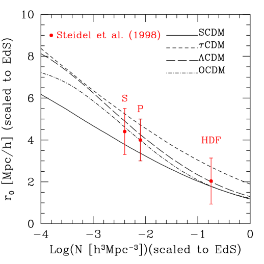
Figure 3: The scaled correlation length [defined as the physical correlation length multiplied by $D_{\star}(1,0)/D_{\star}(\Omega_{0},\Lambda)$ where $D_{\star}(\Omega_{0},\Lambda)$ is the angular size distance at $z=3$] as a function of the scaled abundance [defined as the comoving number density multiplied by $\delta V(\Omega_{0},\Lambda)/\delta V(1,0)$, where $\delta V((\Omega_{0},\Lambda)$ is the comoving volume per unit redshift at $z=3$]. Results are shown for four cosmogonies, as indicated in the panel. Observational data for LBGs to three different limiting magnitudes are taken directly from Steidel et al. (1998b).

The results presented above assume an LBG abundance equal to that in the sample of Adelberger et al. (1998). Observations to fainter magnitude limits will give rise to denser samples, corresponding to less massive and less biased halos. The correlation length is thus predicted to depend on the sample selection criteria. We illustrate this in Figure 3 where we plot the scaled correlation length as a function of the scaled abundance. (The directly observable abundance is the number of LBGs per steradian and per unit redshift, so we normalize the abundances predicted in each cosmology by the appropriate volume per unit redshift. In such a plot the position of the observed data is independent of the cosmology assumed when analysing them.) We show theoretical predictions for four cosmologies with parameters similar to those of the simulation set in Jenkins et al. (1998):

• 1. SCDM: $\Omega_{0}=1.0,\Lambda_{0}=0.0,h=0.5,\Gamma=0.5,\sigma_{8}=0.6$;

  2. $\tau$CDM: $\Omega_{0}=1.0,\Lambda_{0}=0.0,h=0.5,\Gamma=0.2,\sigma_{8}=0.6$;

  3. $\Lambda$CDM: $\Omega_{0}=0.3,\Lambda_{0}=0.7,h=0.7,\Gamma=0.2,\sigma_{8}=1.0$;

  4. OCDM: $\Omega_{0}=0.3,\Lambda_{0}=0.0,h=0.7,\Gamma=0.2,\sigma_{8}=1.0$.

The decrease in correlation length with increasing abundance is quite strong and is very similar in the four cosmologies once they are compared using the scaled variables. We show three observational points taken directly from Steidel et al. (1998b). The point at lowest abundance corresponds to the Adelberger et al. (1998) data discussed above. The next point corresponds to a reanalysis of the projected correlation data in Giavalisco et al (1998). The point at highest abundance comes from an analysis of LBG clustering in the Hubble Deep Field based on photometric redshifts. Clearly all three points are in good agreement with all the models. Again the data provide little discrimination, but seem to provide strong support both to the the hierarchical clustering picture and to the identification of LBGs as the central galaxies of the most massive haloes at $z\sim 3$. For example, if LBGs are assumed to be objects undergoing short-lived bursts with a duty cycle of 10%, then the abundance of host haloes has to be 10 times the observed LBG abundance. Figure 3 shows that the predicted correlation length would then be well below the value measured by Adelberger et al. (1998). As these authors noted in their own analysis, improved measurements of LBG clustering should therefore place interesting constraints on the physical nature of these objects.

2.2 A Model for the Structure of Lyman Break Galaxies

The simple model discussed in the last subsection relates the abundance of LBGs to the mass of their haloes and so is able to predict how they cluster. To study whether other properties of the LBG population, for example their sizes, velocity dispersions and star formation rates, are consistent with the inferred halo masses, we need more detailed models for LBG formation. We develop such a model here based on the disk formation model of Mo, Mao & White (1998, hereafter MMW) and the phenomenological star formation laws of Kennicutt (1998). In §3 we will apply this model to two specific cosmologies, the $\tau$CDM and $\Lambda$CDM models discussed above. The results of the last section can be used to scale the results found there to other cosmologies of interest.

The disk formation model of MMW is an update of the scheme proposed by Fall & Efstathiou (1980, see also Dalcanton, Spergel & Summers 1997, and references therein). This model reproduces the properties of local disk galaxies well, and is consistent with the observed evolution of disk galaxies out to redshifts $\sim 1$ (Mao, Mo & White 1998). The reader is referred to MMW for details; here we only repeat the essentials of the model. Briefly, after the initial protogalactic collapse the gas and dark matter are assumed to be uniformly mixed in a virialized object with density profile,

$$\rho(r)={V_{\rm h}^{2}\over 4\pi Gr^{2}}{1\over\left[\ln(1+c)-c/(1+c)\right]}{r/r_{\rm h}\over(r/r_{\rm h}+1/c)^{2}},$$ (5)

where $V_{\rm h}$ and $r_{\rm h}$ are related to the halo mass $M_{\rm h}$ by equation (2) (Navarro, Frenk & White 1996, 1997, hereafter NFW). The quantity $c$ in equation (5) is known as the halo concentration factor and can be estimated for a halo of given mass in any given cosmogony (see NFW).

As a result of dissipative and radiative processes, the gas component gradually settles into a disk. We assume that the mass of this disk is a constant fraction $m_{d}$ of the halo mass, and that its specific angular momentum is equal to that of the dark halo. These assumptions are questionable but they do reproduce the distribution of disk sizes and masses observed at $z=0$ (see MMW). If the mass profile of the disk is taken to be exponential,

$$\Sigma(r)=\Sigma_{0}\exp(-r/R_{d}),$$ (6)

then $\Sigma_{0}$, $R_{d}$ and the galaxy’s rotation curve are determined uniquely. Specifically,

$$R_{d} = {1\over\sqrt{2}}\lambda r_{\rm h}F_{R}$$ (7)

$$\approx 8.8h^{-1}\,{\rm{kpc}}\left({\lambda\over 0.05}\right)\left({V_{\rm h}\over 250\,{\rm{km\,s^{-1}}}}\right)\left[{H(z)\over H_{0}}\right]^{-1}F_{R},$$

$$\Sigma_{0} = {M_{d}\over 2\pi R_{d}^{2}}$$ (8)

$$\approx 380{M_{\odot}\over{\rm pc}^{2}}h\left({m_{d}\over 0.05}\right)\left({\lambda\over 0.05}\right)^{-2}\left({V_{\rm h}\over 250\,{\rm{km\,s^{-1}}}}\right)\left[{H(z)\over H_{0}}\right]F_{R}^{-2},$$

where $\lambda$ is the spin parameter of the halo and $F_{R}$ is a constant of order unity (see Mao & Mo 1998). From equations (7) and (8) it is clear that high-redshift disks are generically smaller and denser than nearby systems. For example, for fixed $V_{\rm h}$ and $\lambda$, scalelengths are 8 times smaller at $z=3$ than at $z=0$ in an EdS universe; this factor is about 4 for a flat universe with $\Omega_{0}=0.3$.

In systems with $\lambda$ smaller than some critical value, $\lambda_{\rm crit}$, gas cannot settle to a centrifugally supported disk without first becoming self-gravitating. In this case collapse may be arrested by star formation without formation of an equilibrium disk. The size of the galaxy would then reflect the scale at which it became baryon-dominated rather than its angular momentum support. In such cases we assume the final size and density profile of the galaxy to be those that it would have according to our disk model if its halo spin were $\lambda_{\rm crit}$ rather than the actual value $\lambda$. The final configuration is probably spheroidal rather than disk-like in such systems, but this should not seriously affect the size and velocity dispersion estimates given below. The effects on the star formation rate are harder to assess, although we note that the phenomenological model we adopt does seem to describe nearby starbursts where conditions may be similar to those we envisage during the collapse of low spin systems (Kennicutt 1998). For detailed modelling we will take $\lambda_{\rm crit}=m_{d}$, as discussed in MMW.

These assumptions, together with the star formation law which we discuss next, allow us to compute the properties of a newly formed galaxy in any cosmogony for any given set of the parameters, $M_{\rm h}$, $\lambda$ and $m_{d}$. As we will see below, most of our predictions do not depend on the exact value assumed for $m_{d}$, but some, like the star formation rate, vary strongly with this quantity.

We estimate star formation rates using the empirically based Schmidt law proposed by Kennicutt (1998):

$$\Sigma_{\rm SFR}=2.5\times 10^{-4}\left({\Sigma(r)\over 1M_{\odot}{\rm pc}^{-2}}\right)^{1.4}M_{\odot}{\rm~{}yr^{-1}~{}kpc^{-2}},$$ (9)

where $\Sigma_{\rm SFR}$ is the SFR per unit area, and $\Sigma(r)$ is the mass surface density of HI and ${\rm H_{2}}$ gas. This law fits the SFR in nearby galaxies over a total range of more than $10^{7}$ in $\Sigma_{\rm SFR}$ with a scatter of a factor of 2 or 3. We assume $\Sigma(r)$ to be given by equation (6) so our predicted SFR will scale approximately as $m_{d}^{1.5}$. In most of our calculations, we will take $m_{d}=0.03$, but this choice is quite arbitrary. In principle $m_{d}$ could range between 0 and $f_{\rm B}\equiv\Omega_{\rm B}/\Omega_{0}$. A comparison of nucleosynthesis calculations with the abundance of light elements suggests $\Omega_{\rm B}\sim 0.02h^{-2}$ (Schramm & Turner 1998). We assume $m_{d}\ <f_{\rm B}$, because condensation of halo gas into LBGs is likely to be less than 100% efficient. The uncertainty in the appropriate value of $m_{d}$ makes the SFR distribution the least robust of our predictions. We will come back to this issue later.

In hierarchical structure formation, haloes grow continuously by accretion and merging. It is therefore important to examine whether the gas associated with a dark halo has time to cool and settle into a disk before the halo merges into a larger system. This question is best addressed through numerical simulations. The formation of individual galaxies in CDM cosmologies has been simulated by a number of authors (Navarro & White 1994; Navarro, Frenk & White 1995; Haehnelt, Steinmetz & Rauch 1998; Navarro & Steinmetz 1997; Weil, Eke & Efstathiou 1998). These studies all agree that a large fraction of the gas associated with high redshift halos is able to cool and condense into disk-like systems. Furthermore the structure of these disks is reasonably approximated by an exponential law over the bulk of the mass. The outer disk is, however, frequently disturbed by ongoing interactions and mergers, and this results in a cross-section for damped Ly$\alpha$ absorption at $z\sim 2$ which is substantially larger than predicted by an equilibrium disk model (Haehnelt, Steinmetz & Rauch 1998). A further problem is that these simulations all show a substantial transfer of angular momentum from the cool gas to the dark matter. This produces $z=0$ disks which are smaller than observed, and so also smaller than our models predict. The resolution of this difficulty remains unclear (cf. Navarro & Steinmetz 1997; Weil, Eke & Efstathiou 1998). We persevere with our simple models because they do fit observations of nearby galaxies and they are consistent with the observed evolution of disks out to $z\sim 1$.

3 Predictions for the LBG Population

The simple galaxy formation model described above allows us to calculate the properties of the central galaxy in a halo with given mass, spin parameter and redshift. To predict the properties of the LBG population, we also need to know the distributions of $M_{\rm h}$ and $\lambda$ as a function of redshift. As in Section 2, we use the PS formalism to calculate the abundance of dark haloes. $N$-body simulations show the distribution of $\ln\lambda$ for dark haloes is approximately normal with mean ${\overline{\ln\lambda}}=\ln 0.05$ and dispersion $\sigma_{\ln\lambda}=0.5$ (see equation [15] in MMW; Warren et al. 1992; Cole & Lacey 1996; Lemson & Kauffmann 1998). This distribution is found to depend only weakly on cosmology and on the mass and environment of haloes (Lemson & Kauffmann 1998). With the distributions of $M_{\rm h}$ and $\lambda$ given, we can generate Monte Carlo samples of the halo distribution in the $M_{\rm h}-\lambda$ plane at any given redshift. We can then use the galaxy formation model of §2.2 to transform the halo population into an LBG population.

In order to model the observed LBG population, we must incorporate the criteria by which they were selected. We will assume that the colour and magnitude limits of the Steidel et al. sample result in a set of $z\sim 3$ galaxies complete above some limiting star formation rate. This neglects the fact that the magnitude limit (${\cal R}<25.5$, corresponding to a $1500{\rm\AA}$ luminosity limit, $L_{1500}\ga 1.3\times 10^{41}h^{-2}{\rm erg\,s^{-1}\AA^{-1}}$ at $z=3$ in an Einstein-de Sitter universe) may correspond to different SFRs in objects with differing dust distributions or star formation histories (see §3.5). Since the mean conversion from $L_{1500}$ to SFR is controversial, we use the observed abundance of LBGs to set the limiting SFR, checking a posteriori whether the resulting value seems plausible. Specifically, we identify LBGs as the most rapidly star-forming galaxies at $z=3$, subject to the condition that the comoving number density of the model population is the same as that observed. This defines a SFR threshold. This procedure depends on the relation between SFR and the far-UV luminosity only in a loose sense: it is valid provided the uncertainties in the conversion from SFR to far-UV luminosity do not induce a severe mixing between galaxies with different SFR. It also requires that star formation in each LBG last for a period comparable to the Hubble time at $z\sim 3$; otherwise the observed number of LBGs would be smaller than the number of haloes able to host them. As we will see in §3.5, this requirement is indeed fulfilled in our model.

Once the LBG population has been identified in this way in a Monte Carlo simulation of the high-redshift galaxy population, we can study its statistical properties in some detail. For brevity, results are presented below only for the $\tau$CDM and $\Lambda$CDM models, and only for the abundance estimated by Adelberger et al. (1998). The results can be scaled approximately to other models and other abundances by careful use of the results shown in §2.1.

3.1 Halo circular velocities

Figure 4: The circular velocity distribution for the haloes which host LBGs. Solid and dashed histograms are for $\Lambda$CDM and $\tau$CDM, respectively.

Figure 4 shows the distribution of circular velocity for the haloes which host the LBGs. In $\Lambda$CDM, these circular velocities are quite big, with a median of about $290\,{\rm{km\,s^{-1}}}$, corresponding to a total halo mass $M_{\rm h}\sim 1.0\times 10^{12}h^{-1}M_{\odot}$. In this model, LBGs are indeed associated with massive dark haloes. In contrast, the halo circular velocities in the $\tau$CDM model are much smaller. The median is now about $180\,{\rm{km\,s^{-1}}}$, corresponding to $M_{\rm h}\sim 1.5\times 10^{11}h^{-1}$. In this cosmogony, relatively few massive haloes form before $z=3$, and one has to include lower mass systems in order to match the observed number density of LBGs. Note that these median values are quite close to the lower limits inferred for the halo circular velocities using the simpler model of §2.1. In the current model lower mass halos can make it into the sample if they have small $\lambda$ values, since they are then predicted to be compact and to have higher than average SFRs for their mass.

3.2 Correlation functions

At $z=3$ the characteristic mass of dark halos (defined by $\Delta(M_{*})=\delta_{c}(z)$) corresponds to a halo circular velocity $V_{*}\approx 160\,{\rm{km\,s^{-1}}}$ for $\Lambda$CDM and $V_{*}\approx 40\,{\rm{km\,s^{-1}}}$ for $\tau$CDM. Thus the haloes which host the LBG population are much more massive than $M_{*}$, especially in $\tau$CDM, and the distribution of LBGs should be strongly biased relative to that of the mass. The predicted bias factor can be obtained by averaging $b(V_{\rm h},z)$, as given in equation (4) over the $V_{\rm h}$-distribution shown in Fig.4. The result is $b=2.8$ for $\Lambda$CDM and $b=5.0$ for $\tau$CDM. These are similar to the bias factors derived by Steidel et al. (1998a,b; see also Adelberger et al. 1998) for the observed LBGs.

Figure 5: The predicted two-point correlation function for LBGs with the abundance at $z=3$ estimated by Adelberger et al. (1998). Results for $\Lambda$CDM are shown by the solid line and $\tau$CDM by the dashed line. The dotted line is a power law $\xi\propto r^{-1.6}$.

Figure 5 shows the predicted correlation function for LBGs in the $\tau$CDM and $\Lambda$CDM models. In comoving units the correlation length is $r_{0}\approx 4.5\,h^{-1}{\rm{Mpc}}$ for $\tau$CDM, while $r_{0}\approx 5.5\,h^{-1}{\rm{Mpc}}$ for $\Lambda$CDM. These predictions are slightly below those of the simple model of §2.1 as a result of the inclusion of some lower mass haloes. They agree well with the observational result of Adelberger et al. (1998) based on a count-in-cells analysis of a fully spectroscopically confirmed sample. This observational result may still be uncertain, however. For example, Giavalisco et al. (1998) used angular correlation data for a larger and slightly fainter sample of LBGs to infer $r_{0}=(2.1\pm 0.5)\,h^{-1}{\rm{Mpc}}$ at $z=3$ in an Einstein-de Sitter universe. A reanalysis of these same data in Steidel et al. (1998b) gave the intermediate abundance point plotted in Figure 3 which is clearly in much better agreement both with the models and with the Adelberger et al. point. Confirmation of the measured amplitudes in independent data sets would clearly be very valuable.

The present-day descendents of the LBGs will have a correlation function which can be written as

$$\xi_{0}(r)=b_{0}^{2}\xi_{\rm m}(r,0),$$ (10)

where $\xi_{\rm m}(r,0)$ is the present-day mass correlation function, and the bias factor is related to that at the redshift $z$ where the LBGs were identified by

$$b_{0}(V_{\rm h},z) = 1+{1\over\delta_{c}(z)}\left[{\delta_{c}^{2}(z)\over\Delta^{2}(M_{\rm h})}-1\right]$$ (11)

$$= 1+{g(z)\over(1+z)g(0)}\left[b(V_{\rm h},z)-1\right]$$

(Mo & White 1996; Mo & Fukugita 1996). Note that each present-day descendent must be weighted by the number of LBGs it contains when estimating these correlations. The detailed models of Baugh et al. (1998) suggest that most descendents contain only a single LBG. Using the values of $b$ estimated above, we obtain $b_{0}=1.6$ for $\Lambda$CDM and $b_{0}=2.0$ for $\tau$CDM. Normal bright galaxies at $z=0$ have $b\sim\sigma_{8}^{-1}$. The correlation amplitude for LBG descendents is thus predicted to exceed that of normal bright galaxies by a factor of about $(\sigma_{8}b_{0})^{2}$, or $\sim 2.5$ for $\Lambda$CDM and $\sim 1.4$ for $\tau$CDM. This is consistent with the conclusions of Mo & Fukugita (1996), Baugh et al. (1998) and Governato et al. (1998); LBG descendents are primarily among the brightest galaxies and are found preferentially in clusters.

3.3 Half-light radii

Figure 6: The distribution of half-light radii for LBGs. In each panel the solid histogram gives the model prediction and the dashed histogram shows observational data (cf. table 2 in Giavalisco, Steidel, & Macchetto 1996 and table 2 in Lowenthal et al. 1997).

Figure 7: The spin parameter distribution for the haloes which host LBGs (solid curve) is compared to that for haloes which host damped Ly$\alpha$ absorption systems (DLSs, dashed curve). Note that while LBGs are biased towards haloes with low spin, DLSs are biased towards haloes with high spin.

Figure 6 shows the predicted distribution of effective radius, $R_{\rm eff}$, for the LBG population. We define $R_{\rm eff}$ as the semimajor axis of the isophote which contains half of the star formation activity. This is easily calculated from our model and will coincide with the size of the region containing half the observed light provided the relation between SFR and far-UV surface brightness does not vary much across a galaxy. Half-light radii are predicted to be quite small. The median $R_{\rm eff}$ is about $2\,{h^{-1}{\rm kpc}}$ for $\Lambda$CDM , while it is only $0.6\,{h^{-1}{\rm kpc}}$ for $\tau$CDM. This large difference arises because host halos are less massive and $H(z)/H_{0}$ is larger in in $\tau$CDM than in $\Lambda$CDM [see equation (2)]. Although partially offset by the fact that angular size distances are larger in the low density case, it opens the possibility that size measurements for LBGs might significantly constrain cosmological parameters.

HST imaging of LBGs (to a magnitude limit comparable to ${\cal R}=25.5$) in the Hubble Deep Field by Lowenthal et al. (1997) gave values of $R_{\rm eff}$ in the range $(0.5\to 2.1)\,{h^{-1}{\rm kpc}}$, with a median near $1.1\,{h^{-1}{\rm kpc}}$, under the assumption of an Einstein-de Sitter universe. The corresponding range is $(0.8\to 3.6)\,{h^{-1}{\rm kpc}}$, with a median near $1.8\,{h^{-1}{\rm kpc}}$, for a flat universe with $\Lambda=0.3$. Similar results were obtained by Giavalisco, Steidel & Macchetto (1996). These data agree well with our models for $\Lambda$CDM, but are perhaps somewhat larger than predicted for $\tau$CDM. The observational data are still quite sparse, and larger and more complete samples are needed to get reliable constraints.

The small sizes predicted for LBGs may appear surprising given the large circular velocities predicted for their halos. For given $V_{\rm h}$, halo size decreases with $z$ as $H^{-1}(z)$ (cf. equation 2). At $z=3$ this gives a factor of 8 in an Einstein-de Sitter universe and a factor of $4$ in a flat universe with $\Omega_{0}=0.3$. In our model, the ratio of galaxy size to halo size depends only on $\lambda$ and is independent of $z$. The small sizes of the LBGs are due mostly to the small size of their haloes, but also to the fact that, since we select LBGs according to SFR, they are biased towards haloes with small $\lambda$; smaller $\lambda$ gives higher surface density (and so higher SFR) but smaller size. This bias is most clearly shown in Figure 7, where we show the spin parameter distribution for the LBG population. The distribution of $\ln\lambda$ is approximately normal with ${\overline{\ln\lambda}}=\ln 0.035$ and $\sigma_{\ln\lambda}=0.4$. This should be compared with the original distribution which had ${\overline{\ln\lambda}}=\ln 0.05$ and $\sigma_{\ln\lambda}=0.5$.

3.4 Stellar velocity dispersions

Figure 8: The line-of-sight stellar velocity dispersion distribution of LBGs. Solid and dashed histograms are for $\Lambda$CDM and $\tau$CDM, respectively.

Although our models predict the circular velocities of the haloes hosting LBGs to be quite big (cf. Fig. 4), the stellar velocity dispersions of the LBGs themselves can be substantially smaller. This is a result of a combination of projection effects with the fact that the observed stellar distribution samples only the very central regions of the halo potential well. To show this we construct the distribution of SFR-weighted line-of-sight velocity dispersion for our Monte Carlo samples of model LBGs. For a disc galaxy seen at inclination $i$, this dispersion is defined as

$$\sigma_{V}^{2}={1\over 2M_{\rm SFR}}\int_{0}^{\infty}V_{\rm rot}^{2}(r)\sin^{2}(i)~{}\Sigma_{\rm SFR}(r)2\pi rdr,$$ (12)

where the star formation surface density $\Sigma_{\rm SFR}(r)$ is obtained from equations (6) to (9), $M_{\rm SFR}\equiv\int_{0}^{\infty}\Sigma_{\rm SFR}(r)2\pi rdr$, $V_{\rm rot}(r)$ is the disk rotation curve, and $i=0$ refers to a face-on disc. In our Monte Carlo samples we assume $\sin(i)$ to be uniformly distributed on $[0,1]$ corresponding to randomly oriented galaxies. For the ‘spheroid’ population discussed in Section 2.2 (i.e. for systems with $\lambda<\lambda_{\rm crit}$), we assume the stars to be in random motion, with line-of-sight velocity dispersion given by

$$\sigma_{V}^{2}={1\over 3M_{\rm SFR}}\int_{0}^{\infty}V_{\rm rot}^{2}(r)\Sigma_{\rm SFR}(r)2\pi rdr,$$ (13)

where $V_{\rm rot}(r)$ and $\Sigma_{\rm SFR}(r)$ are calculated as for disks but assuming $\lambda=\lambda_{\rm crit}$ rather than the true value. Figure 8 shows the resulting $\sigma_{V}$ distribution for our Monte Carlo samples of LBGs. Comparing this figure with Fig.4 it is clear that stellar velocity dispersions are typically much smaller than halo circular velocities. The median values of $\sigma_{V}$ are $\sim 120\,{\rm{km\,s^{-1}}}$ for $\Lambda$CDM and $\sim 70\,{\rm{km\,s^{-1}}}$ for $\tau$CDM. Much of this reduction is a result of the bulk of star formation occurring on the inner rising part of the disk rotation curve. The values would thus be even smaller if observations were assumed to sample only the inner part of the light distribution. These results suggest that even if stellar velocity dispersions could be reliably measured for LBGs, it would be difficult to use them to infer the mass of the associated halo.

Based on the Ly$\alpha$ emission line widths observed in six LBGs, Lowenthal et al. (1997) inferred $100\,{\rm{km\,s^{-1}}}<\sigma_{V}<230\,{\rm{km\,s^{-1}}}$ with a median $\sim 140\,{\rm{km\,s^{-1}}}$. On the basis of this they argued that LBGs are likely to be the low-mass, star-bursting building blocks of present-day galaxies. A rather different interpretation appears natural in our model. The observed velocity dispersions agree well with what we would predict for LBGs in a $\Lambda$CDM cosmology, and appear too large to be consistent with $\tau$CDM. These values would seem to require LBGs to be the central galaxies in haloes with mass $\sim 10^{12}M_{\odot}$. It would be wrong to put much weight on this conclusion, however, since it is now clear that the widths of the Ly$\alpha$ lines in LBGs are often substantially affected by radiative transfer effects and by non-gravitational motions in the emitting gas; as a result they may bear little relation to the stellar velocity dispersion of the underlying galaxy (Pettini et al. 1998).

Measurement of emission line widths in the near infrared may provide a more reliable estimate of the virial velocity dispersion within LBGs. Results for five galaxies are reported by Pettini et al. (1998) based on UKIRT observations of the ${\rm H}\beta$ and [OIII] emission lines. For four galaxies they find $\sigma_{V}\sim 70\,{\rm{km\,s^{-1}}}$, while for the fifth $\sigma_{V}\sim 200\,{\rm{km\,s^{-1}}}$. The lower values agree well with our $\tau$CDM predictions, but seem on the small side to be consistent with $\Lambda$CDM. On the other hand, a value as large as $200\,{\rm{km\,s^{-1}}}$ is predicted to be very rare in $\tau$CDM and also quite unusual in $\Lambda$CDM. Clearly the observed sample is too small to draw reliable conclusions, and the relation of these linewidths to the underlying stellar velocity dispersion, while probably simpler than that for the Ly$\alpha$ line, is still open to question. In this context, it is interesting to note that in nearby starburst galaxies the velocity dispersions inferred from forbidden emission lines are substantially smaller than the rotation velocities of the host galaxies (e.g. Lehnert & Heckman 1996). This appears to reflect the concentration of star formation to the nuclear regions where the rotation curve is still rising, and so is an example of the effect which leads us to predict LBG velocity dispersions much smaller than the circular velocities of their haloes.

3.5 SFR functions

Figure 9: The star formation rate function (proportional to the UV luminosity function) for LBGs in our $\Lambda$CDM and $\tau$CDM models. The bold histogram in each case is for our standard disk mass fraction $m_{d}=0.03$. The two light histograms are for $m_{d}=0.015$ (left) and $m_{d}=0.06$ (right), respectively.

The UV spectra of LBGs are dominated by the integrated continuum of O and early B stars. Since these stars have short lifetimes, the observed UV luminosity is directly determined by the star formation rate. The main uncertainties in the conversion between these two quantities come from the poorly constrained shape of the stellar Initial Mass Function and, especially, from the difficulties in establishing appropriate corrections for the amount of obscuration by dust. For given halo mass, halo spin parameter and disk mass fraction, our model uniquely predicts the disk surface density (see equations [6-8]). The star formation rate can then be determined as a function of radius (and so integrated over the galaxy as a whole) using equation (9) under the assumption that the disk is (at least initially) fully gaseous. Thus we can determine the abundance of galaxies according to their SFR in our Monte Carlo samples of LBGs. Such functions are shown in Figure 9 for $\Lambda$CDM and $\tau$CDM, and for three choices of the disk mass fraction.

Figure 9 shows clearly that the SFR functions depend strongly on $m_{d}$. This is in contrast to the properties discussed in earlier sections which vary quite weakly with $m_{d}$ over the range considered here – with increasing $m_{d}$ galaxies become somewhat more compact and their internal velocities increase. If we take $m_{d}=0.03$, the limiting SFR for $\tau$CDM is about 10${M_{\odot}\rm yr^{-1}}$ and values up to 200${M_{\odot}\rm yr^{-1}}$ are found in our Monte Carlo samples. Doubling $m_{d}$ increases the cut-off SFR to 30${M_{\odot}\rm yr^{-1}}$ and the largest values to $\sim 400{M_{\odot}\rm yr^{-1}}$. Larger values are found in the $\Lambda$CDM case. For $m_{d}=0.03$ the cut-off occurs near 60${M_{\odot}\rm yr^{-1}}$ and the largest values approach 500 ${M_{\odot}\rm yr^{-1}}$. For $m_{d}=0.06$ the corresponding numbers are 120${M_{\odot}\rm yr^{-1}}$ and 800${M_{\odot}\rm yr^{-1}}$. The larger rates for $\Lambda$CDM reflect the fact that LBGs are hosted by more massive haloes in this model.

For comparison, for a standard IMF and without any correction for obscuration the UV luminosities of the LBGs studied by Steidel et al. (1998a,b) correspond to star formation rates in the range $4-50{M_{\odot}\rm yr^{-1}}$. The corrected rates depend significantly on the extinction law assumed and on the detailed interpretation of the data. Steidel et al (1998) obtained a mean correction of 2.0 and a range of corrected values $4-120{M_{\odot}\rm yr^{-1}}$ for an assumed SMC extinction law, while for the extinction law of Calzetti (1997) they found a mean correction of 7.7 and a range $4-1500{M_{\odot}\rm yr^{-1}}$. Pettini et al. (1998) concluded from their IR observations of a few galaxies that the second of these corrections may be closer to the truth (see also Meurer 1997). All the rates quoted here assume an Einstein-de Sitter cosmology with $h=0.5$. For our $\Lambda$CDM parameters they need to be increased by a factor of 2.5. Figure 9 shows that any of these ranges can be accommodated in either of our models for a plausible choice of $m_{d}$. Recall that taking $m_{d}$ to be constant is a simplification of convenience, and that in practice a range of values (including, perhaps, a systematic dependence on halo mass) is to be expected. Once $m_{d}$ is chosen to match the observed limiting UV luminosities, the SFR functions in Fig. 9 give a good fit to the LBG luminosity function constructed by Dickinson (1998).

If we divide the disk masses of our model LBGs by their inferred SFRs the resulting decay time constant for the star formation is typically 30% of the age of the universe at $z=3$. This is comparable to the timescale on which the LBG halos double their mass, and so to that on which new gas can be supplied. Thus there does not appear to be a “gas supply” problem in the models, and there is no need to invoke a bursting mode for the observed star formation (cf. Lowenthal et al. 1997; Somerville, Primack & Faber 1998).

3.6 Connection to high-redshift damped Ly$\alpha$ systems

As can be seen from Fig 7, the LBG population in our model is biased towards objects with small angular momentum; these have higher surface densities and so higher star formation rates. In contrast the cross-section for damped Ly$\alpha$ absorption by equilibrium disks is dominated by objects with large angular momentum, since the cross-sections of individual objects scale as $\pi R_{d}^{2}\propto\lambda^{2}$ (see MMW). We illustrate this in Fig.7 by overplotting the distribution of $\lambda$ predicted for a population of equilibrium disks selected according to their damped Ly$\alpha$ cross-section. As emphasised most recently by Prochaska & Wolfe (1997), matching the total observed cross-section for damped absorption in this model seems to require the inclusion of systems with rotation speeds too small to be consistent with the observed velocity widths of the associated low ionization metal line systems. Haehnelt, Steinmetz & Rauch (1998) demonstrate that this discrepancy is plausibly eliminated when proper account is taken of the fact that hierarchical formation models predict the outer parts of many high-redshift disks to be both spatially and kinematically distorted by interactions and mergers. This increases both their cross-sections and their line widths. Since the susceptibility to tidal distortion increases with disk size (e.g. Springel & White 1998) it is reasonable to suppose that the bias of such tidally distorted systems towards large $\lambda$ is at least as strong as our predictions for equilibrium disks

The median spin parameters for the LBGs and the damped Ly$\alpha$ systems (DLSs) in Fig 7 are 0.035 and 0.08, respectively. There are essentially no LBGs with $\lambda>0.1$ while nearly $\sim 40\%$ of DLSs have $\lambda>0.1$. Even without accounting for the loss of gas through star formation, the total cross-section of the LBG population for damped absorption is only about one fifth of that of the DLS population to the same mass limit. Since the star formation rate per unit area is $\propto\Sigma^{1.4}\propto\lambda^{-2.8}$, the SFR per unit area in DLSs is, on average, a factor of $\sim 10$ lower than in LBGs. As a result most DLSs will not resemble the bright and compact LBGs, although some may be detected as gas discs with faint LBGs at their centres. We thus predict LBGs and DLSs to be quite distinct populations. Because of their more rapid star formation, LBGs should have systematically higher metallicity and dust content than DLSs. Simple attempts to make direct connections between these two populations are therefore dangerous. For example, it may be misleading to compare the metallicities of DLSs directly with those of LBGs (Madau, Pozzetti & Dickinson 1998).

3.7 Discs or spheroids?

In Section 2.2 we suggested that LBGs in high spin haloes may be rotationally supported disks, while those in low spin haloes may be (partially) supported by random motions. Stars in the latter systems may form before the gas can settle to centrifugal equilibrium and so may produce spheroids. In reality, we might expect to see the whole spectrum from completely rotationally supported discs, through partially rotationally supported disc/bulge systems, to random-motion supported spheroids. This would be reflected in a variety of shapes in the images of LBGs. If it is correct, as we have argued, that observed LBGs are predominantly in low-spin haloes, they should be biased towards spheroids, and so should appear more compact and less flattened than the general population. According to our crude stability criterion, the fraction of the population in “spheroids” is given roughly by the condition $\lambda<m_{d}$. Thus, if $m_{d}>0.035$, the majority of LBGs may be spheroidal. Unfortunately, these arguments are quite sketchy, and reliable quantitative predictions will require detailed and convincing simulations of how gas settles and forms stars in these objects.

4 Discussion

In this paper, we have modeled both the clustering and the internal structure of the recently discovered population of Lyman break galaxies. The assumption that these objects are the central galaxies of massive halos allows models which fit the structural and star formation properties of nearby spirals to be scaled to $z\sim 3$. The populations observed by Steidel et al. (1998a,b) and Adelberger et al. (1998) can then be identified as the most rapidly star-forming (and hence brightest) galaxies, and the conversion between star formation rate and UV luminosity can be set so that the predicted LBG abundance equals that observed. For given cosmological parameters the models then predict distributions of size, velocity dispersion, and star-formation rate for the observed samples, as well as the strength of their clustering. A reasonable fit to the current data can be found in all currently popular cosmologies.

The models predict that Lyman break galaxies and damped Ly$\alpha$ absorbers should form almost disjoint populations. These two kinds of object are currently the best available tracers of galaxy formation at high redshifts. However, LBG samples are biased in favour of systems of low angular momentum, and so high star formation rate, while DLS samples are biased in favour of systems of high angular momentum, and so large absorption cross-section. This results in substantial systematic differences in size, kinematics and star formation history. Most LBGs should be compact, high surface brightness, possibly spheroidal systems, whereas most DLSs should be extended, low surface brightness, rotationally supported disks. The difference in star formation rates will plausibly cause the LBGs to have significantly higher metal abundances than the DLSs. Direct observation of these differences would provide important evidence for the picture we have developed.

Because we do not attempt any explicit modelling of the cooling and feedback processes associated with galaxy formation, we treat the mass fraction which settles to the halo centre as an adjustable constant. In addition we assume the specific angular momentum of the central galaxy to be the same as that of its halo. These are probably the most questionable aspects of our models. In Mo, Mao & White (1998) we showed that these simple assumptions provide a surprisingly good fit to the properties of local spirals, and in Mao, Mo & White (1998) that they are also consistent with the available data on the evolution of disks out to $z\sim 1$. This does not, of course, imply that they must be good assumptions also for LBGs at $z\sim 3$. Our predictions for sizes, dispersion velocities and clustering depend only weakly on disk mass fraction, and the clustering predictions are also nearly independent of the assumed specific angular momentum. On the other hand, the predicted star formation rates depend strongly on both assumptions. The observed clustering of LBGs should thus be considered a robust confirmation of hierarchical galaxy formation theory and of the assumption that the LBGs in current spectroscopic samples are primarily the dominant galaxies of the most massive haloes at $z\sim 3$. Our predictions for sizes and velocity dispersions are also reasonably robust provided angular momentum transfer is no more efficient in LBG formation than at low redshift. The agreement between models and observational data provides significant further confirmation of the basic paradigm. For the star formation rates we are reduced to noting that the observed UV luminosity functions can be matched for any of the mean obscuration factors currently under debate using physically plausible values of $m_{d}$, the LBG mass fraction.

The model we propose differs significantly from the low-mass starburst scenario suggested by Lowenthal et al. (1997). In this scenario, star formation in each LBG lasts for less than $10^{8}$ yr, so the observed objects are only a small fraction ($\la 10\%$) of the total (bursting plus dormant) population. If the abundance of potential LBGs is at least ten times the value we have adopted, and if again LBGs are assumed to be the dominant objects in their haloes, then substantially lower mass haloes must be able to host LBGs. This results in reductions of the limiting halo circular velocity (and so of the predicted sizes and velocity dispersions) by a factor of 2 or more, and of the predicted clustering length by a factor of at least 1.6. Such reductions make the apparent agreement with observation significantly worse, particularly for $\tau$CDM where they appear to be excluded by the observed sizes and velocity dispersions. Clearly better determinations of $r_{0}$, $R_{\rm eff}$ and $\sigma_{V}$ should decide definitively between the two models.

In recent work Somerville, Primack & Faber (1998) have suggested a variant of this starburst picture in which observed LBGs are no longer assumed to be the dominant galaxies in their haloes but are taken to be satellite systems undergoing interaction-induced starbursts in relatively massive haloes. Our modelling suggests several difficulties with this picture. We would again predict the sizes and velocity dispersions of these low-mass objects to be quite small in comparison with the current data. In addition, if on average there is one bursting object per massive halo (so that large-scale clustering is the same as in our model and so in agreement with the data) then Poisson statistics predict that more than half the LBGs should share their halo with a second observable object, whereas the number of close pairs ($\Delta r_{p}\la 100\,{h^{-1}{\rm kpc}}$) is very small in the observed samples (Giavalisco et al. 1998). If bursting satellites can occur in lower mass haloes, thus reducing the mean number per halo and so the probability of multiple objects, then the clustering strength is also reduced as before. Finally, current semi-analytic models suggest that in galaxy mass halos the amount of fuel available for star formation in the central object is considerable larger than that available in all the satellites combined (Kauffmann et al. 1993; Baugh et al. 1998; Governato et al. 1998). A bursting satellite model then requires a substantial fraction of the observed star formation at $z\sim 3$, and in particular the most luminous starbursts, to be occurring in objects with a small fraction of the total available fuel.

In conclusion, a model in which current spectroscopic samples of Lyman break galaxies are dominated by the central galaxies of the most massive haloes at $z\sim 3$ seems to account in a simple and consistent way for the sizes, velocity dispersions, star formation rates and clustering of these objects. The current rather sparse data appear to favour such models over alternatives in which the galaxies are assumed to be undergoing short-lived starbursts.

References

- [1] Adelberger K. L.,Steidel, C.C., Giavalisco M., Dickinson M. E., Pettini M., Kellogg M. 1998, preprint (astro-ph/9804236)
- [2] Bagla J.S., 1998a, MNRAS, 297, 251
- [3] Bagla J.S., 1998b, preprint (astro-ph/9711081)
- [4] Baugh C.M., Cole S., Frenk C.S., Lacey C.G. 1998, ApJ, 498, 504
- [5] Blumenthal G.R., Faber S.M., Primack J.R., Rees M.J. 1984, Nature, 311, 517
- [6] Calzetti D., 1997, AJ, 113, 162
- [7] Cole S., Aragon-Salamanca A., Frenk C.S., Navarro J.F., Zepf S. E., 1994, MNRAS, 271, 781
- [8] Cole S., Lacey C., 1996, MNRAS, 281, 716
- [9] Coles P., Lucchin F., Matarrese S., Moscardini L. 1998, preprint (astro-ph/9803197)
- [10] Dalcanton J.J., Spergel D.N., Summers, F.J., 1997, ApJ, 482, 659
- [11] Davis M., Efstathiou G., Frenk C.S., White, S.D.M., 1985, ApJ, 292, 371
- [12] Dickinson M., 1998, preprint (astro-ph/9802064)
- [13] Fall S.M., Efstathiou G., 1980, MNRAS, 193, 189
- [14] Giavalisco M., Steidel C.C., Macchetto F. D. 1996, 470, 189
- [15] Giavalisco M., Steidel, C.C., Adelberger K. L., Dickinson M. E., Pettini M., Kellogg M. 1998, preprint (astro-ph/9802318)
- [16] Governato F., Baugh C.M., Frenk C. S., Cole S., Lacey C.G., Quinn T., Stadel J. 1998, preprint (astro-ph/9803030)
- [17] Haehnelt, M.G., Steinmetz M., Rauch M. 1998, ApJ, 495, 647
- [18] Jain B., Mo H. J., White, S. D. M., 1995, MNRAS, 276, L25
- [19] Jenkins A., Frenk C.S., Pearce F.R., Thomas P.A., Colberg, J.M., White S.D.M., Couchman H.M.P., Peacock J.A., Efstathiou G., Nelson A.H., 1998, ApJ, 499, 20
- [20] Jing Y.P., 1998, preprint (astro-ph/9805202)
- [21] Jing Y.P., Suto Y., 1998, ApJ, 494, L5
- [22] Kauffmann G., White S.D.M., Guiderdoni B., 1993, MNRAS, 264, 201
- [23] Katz N., Hernquist L., Weinberg D.H., 1998, preprint (astro-ph/9806257 )
- [24] Kennicutt R., 1998, preprint (astro-ph/9712213)
- [25] Lemson G., Kauffmann G. 1998, preprint (astro-ph/9710125)
- [26] Lehnert M.D., Heckman T.M., 1996, ApJ, 472, 546
- [27] Lowenthal J.D., Koo D.C. Guzmán R., Gallego J., Phillips A.C., Faber S.M., Vogt, N.P., Illingworth G.D. 1997, ApJ, 481, 67
- [28] Madau P., Pozzetti L., Dickinson M., 1998, ApJ, 498, 106
- [29] Mao S., Mo H.J., 1998, MNRAS, 296, 847
- [30] Mao S., Mo H.J., White S.D.M., 1998, MNRAS, 297, 71
- [31] Meurer, G. R. 1997, preprint (astro-ph/970816)
- [32] Mo H.J., Fukugita M., 1996, ApJ, 467, L9
- [33] Mo H.J., Jing Y.P., Börner G., 1997, MNRAS, 286, 979
- [34] Mo H.J., Mao S., White S.D.M., 1998, MNRAS, 295, 319 (MMW)
- [35] Mo H.J., White S.D.M., 1996, MNRAS, 282, 347
- [36] Moscardini L., Coles P., Lucchin F., Matarrese S. 1998, preprint (astro-ph/9712184)
- [37] Navarro J.F., Steinmetz M., 1997, ApJ, 478, 13
- [38] Navarro J.F., White, S.D.M., 1994, MNRAS, 267, 401
- [39] Navarro J.F., Frenk, C. S., White, S.D.M., 1995, MNRAS, 274, 755
- [40] Navarro J.F., Frenk, C. S., White, S.D.M., 1996, ApJ, 462, 563
- [41] Navarro J.F., Frenk, C. S., White, S.D.M., 1997, ApJ, 490, 49 (NFW)
- [42] Peacock J. A., Dodds S.J., 1996, MNRAS, 280, L19
- [43] Peacock J. A., Jimenez R., Dunlop J.S., Waddington I., Spinrad H., Stern D., Dey A., Windhorst R.A., 1998, preprint (astro-ph/9801184)
- [44] Pettini M., Steidel C.C., Dickinson M. E., Kellogg M., Giavalisco M., Adelberger K. L., 1998, preprint (astro-ph/9707200)
- [45] Press W.H., Schechter P., 1974, ApJ, 187, 425 (PS)
- [46] Prochaska J.X., Wolfe A.M., 1997, 487, 73
- [47] Schramm, D. N., Turner M. S., 1998, Rev. Mod. Phys. 70, 303
- [48] Sommerville R.S., Primack J.R., Faber S.M., 1998, preprint (astro-ph/9806228)
- [49] Springel V., White S.D.M., 1998, preprint (astro-ph/9807320)
- [50] Steidel C. C., Pettini M., Hamilton D., 1995, AJ, 110, 2519
- [51] Steidel C. C., Giavalisco M., Pettini M., Dickinson, M., Adelberger K. L. 1996, ApJ, 462, L17
- [52] Steidel C. C., Adelberger K. L., Dickinson M., Giavalisco M., Pettini M., Kellogg M., 1998a, ApJ, 492, 428
- [53] Steidel C., Adelberger K. L., Giavalisco M., Dickinson M., Kellogg M. 1998b, preprint (astro-ph/9805267)
- [54] Viana P. T. P., Liddle A. R., 1996. MNRAS, 281, 323
- [55] Warren M.S., Quinn P.J., Salmon J.K., Zurek W.H., 1992, ApJ, 399, 405
- [56] Wechsler R.H., Gross M.A.K., Primack J.R., Blumenthal G.R., Dekel A. 1998, preprint (astro-ph/9712141)
- [57] Weil M.L., Eke V.R., Efstathiou G., 1998, preprint (astro-ph/9802311)
- [58] White S.D.M., Frenk C.S., 1991, ApJ, 379, 52
- [59] White S.D.M., Efstathiou G., Frenk C., 1993, MNRAS, 262, 1023
- [60] White S.D.M., Rees M.J., 1978, MNRAS, 183, 341