Tidal tails in CDM cosmologies

Abstract

We study the formation of tidal tails in pairs of merging disk galaxies with structural properties motivated by current theories of cold dark matter (CDM) cosmologies. In a recent study, Dubinski, Mihos & Hernquist (1996) showed that the formation of prominent tidal tails can be strongly suppressed by massive and extended dark haloes. For the large halo-to-disk mass ratio expected in CDM cosmologies their sequence of models failed to produce strong tails like those observed in many well-known pairs of interacting galaxies. In order to test whether this effect can constrain the viability of CDM cosmologies, we construct N-body models of disk galaxies with structural properties derived in analogy to the analytical work of Mo, Mao & White (1998). With a series of self-consistent collisionless simulations of galaxy-galaxy mergers we demonstrate that even the disks of very massive dark haloes have no problems developing long tidal tails, provided the halo spin parameter is large enough. We show that the halo-to-disk mass ratio is a poor indicator for the ability to produce tails. Instead, the relative size of disk and halo, or alternatively, the ratio of circular velocity to local escape speed at the half mass radius of the disk are more useful criteria. This result holds in all CDM cosmologies. The length of tidal tails is thus unlikely to provide useful constraints on such models.

1 Introduction

In standard hierarchical scenarios for galaxy formation, mergers of galaxies are common events that lead to the build-up of ever more massive galaxies. In fact, such mergers have been observed for a long time. There is now a large database of well studied examples of merging or strongly interacting disk galaxies, among the most prominent of them are NGC4038/39 (the Antennae), NGC4676 (the Mice), and NGC7252. Many of these pairs feature extended tidal tails, with a length that can reach more than 100$\,h^{-1}{\rm kpc}$ in projection, or in the extreme case of IRAS19254-7245 (the Superantennae) even $\sim 305\,h^{-1}{\rm kpc}$ from tip to tip (Colina et al. 1991).

The tails originate in close encounters of disk galaxies, when the mutual tidal field ejects disk stars into arcing trajectories that lead to the formation of long tails pointing way from the galaxies, and of bridges connecting them. This process was first demonstrated convincingly in a classic paper by Toomre & Toomre (1972). Later White (1978, 1979) computed the first fully self-consistent 3-dimensional simulations of merging galaxies and established the rapidity of the orbital decay, and the structural resemblence of the merger remnants to elliptical galaxies. This work has been confirmed and extended over the years by simulations with increasingly realistic initial conditions and ever better numerical resolution (Farouki & Shapiro 1982; Farouki et al. 1983; Negroponte & White 1983; Barnes 1988, 1989, 1992; Hernquist 1992, 1993b; Barnes & Hernquist 1996). There have also been quite successful attempts to model particular interacting systems in detail, for example NGC7252 (Hibbard & Mihos 1995) and NGC2442 (Mihos & Bothun 1997).

Recently, Dubinski, Mihos & Hernquist (1996, hereafter DMH) studied the morphology of tidal tails in a series of merging models of disk galaxies with varying halo-to-disk mass ratio. In their sequence of four models, they kept the inner rotation curve very nearly constant and surrounded the disk and the bulge with ever more extended and massive dark haloes. They found that with increasing mass of the dark halo, the resulting tidal tails became shorter and less massive. Their explanation for this effect is simple. For a fixed structure of the disk, a more massive halo leads to a deeper potential well and a higher encounter velocity. As a consequence, the duration and overall strength of the perturbation to the disk is smaller, and the perturbed material cannot as easily climb out of the deeper potential well.

Dubinski, Mihos, and Hernquist have followed up this study with an analysis of NGC7252 (Mihos et al. 1998), and an investigation of different dark matter profiles with a restricted 3-body code (Dubinski et al. 1997). Again they found that disk models with large halo-to-disk mass ratio were not able to produce prominent tidal tails. In particular, they concluded that for mass ratios above 10:1 it should be exceedingly difficult to make tails as long as those observed in systems like NGC7252 or NGC4038/39. Since the currently favoured theoretical values of halo-to-disk mass are considerably higher than this, they speculated that there might be a conflict with cold dark matter (CDM) cosmologies.

In this work we examine the tail-forming ability of realistic models of disk galaxies, where ‘realistic’ means that their structural properties are motivated to a large degree by current theories of CDM cosmologies. We derive the structural properties of our disk galaxies according to the analytic model of Mo, Mao & White (1998, hereafter MMW), and we collide pairs of these galaxies in self-consistent N-body simulations. We adopt initial conditions for these merger simulations that are favourable for tail formation.

We will demonstrate that the halo-to-disk mass ratio is not a particularly useful parameter for characterizing ability to make tidal tails. We find that it is the relative distribution of disk and halo material that is relevant, not the mass ratio itself. This conclusion was reached earlier by Barnes (1997, private communication) through analysis of a series of simulations with halo/disk models differing both from those of DMH and from the CDM-based models we use here.

We will show that realistic disk models in CDM cosmologies have no problem producing long and massive tidal tails, provided the spin parameter of their dark halo is large enough. This result is practically independent of the adopted halo-to-disk mass ratio.

This work is organized as follows. In Section 2 we describe the structural properties of our disk models, and in Section 3 we discuss our techniques for setting up N-body representations of these models. A description of the different simulations we have performed is given in Section 4, while Section 5 presents the results. Finally, we summarize and discuss our findings in Section 6.

2 Models of disk galaxies

MMW have developed an analytical model for the structure of disk galaxies embedded in cold dark matter haloes. Their model rests on a number of simple yet plausible assumptions, and it is very successful in reproducing the observed properties of disk galaxies. In particular, the predicted population can match the slope and scatter of the Tully-Fisher relation as well as the properties of damped Ly$\alpha$ absorbers in QSO spectra. We take their model as basis to derive the structural properties of our N-body models of disk galaxies. For definiteness, we briefly summarize the relevant assumptions and equations.

2.1 Dark haloes

Using high-resolution N-body simulations, Navarro, Frenk & White (1996, 1997, hereafter NFW) established that haloes formed by the gravitational clustering of cold dark matter exhibit a universal structure. Suitably scaled, the density distribution of these dark matter haloes does not depend on cosmology. The NFW-profile is given by

$$\rho(r)=\rho_{\rm crit.}\frac{\delta_{\rm c}}{({r}/{r_{\rm s}})\left(1+{r}/{r_{\rm s}}\right)^{2}},$$ (1)

where $\rho_{\rm crit.}$ is the background density at the time of the halo formation, $r_{\rm s}$ is a scale radius, and $\delta_{\rm c}$ is a characteristic overdensity. Note that the slope of this profile is shallower than isothermal at the center, and it gradually steepens outward to an asymptotic slope of $-3$. Following NFW, we define the virial radius $r_{200}$ as the radius with mean overdensity 200, i.e. it contains the virial mass

$$M_{200}\equiv 200\rho_{\rm crit.}\,\frac{4\pi}{3}r_{200}^{3}\,,$$ (2)

and we define the concentration

$$c\equiv\frac{r_{200}}{r_{\rm c}}$$ (3)

of the halo. With these definitions, the characteristic overdensity is given by

$$\delta_{\rm c}=\frac{200}{3}\,\frac{c^{3}}{\ln(1+c)-\frac{c}{1+c}}.$$ (4)

Further, let

$$v_{200}^{2}\equiv\frac{GM_{200}}{r_{200}}$$ (5)

be the circular velocity at the virial radius. Given the concentration $c$ and the Hubble constant $H(z)$, the radial density profile of a halo may then be specified by anyone of the parameters $v_{200}$, $r_{200}$, or $M_{200}$. In particular, we have

$$M_{200}=\frac{v_{200}^{3}}{10GH(z)},\;\;\;\;\mbox{and}\;\;\;\;\;r_{200}=\frac{v_{200}}{10H(z)}.$$ (6)

2.2 Putting a disk into the halo

We now put a stellar disk into an NFW halo according to the model of MMW. This rests on four key assumptions:

1. The mass $M_{\rm d}$ of the disk is a given fraction $m_{\rm d}$ of the halo mass.

2. The spin $J_{\rm d}$ of the disk is a given fraction $j_{\rm d}$ of the angular momentum $J$ of the halo.

3. The disk has the structure of a thin exponential disk, and it is cold and centrifugally supported.

4. Only disks that are dynamically stable against bar formation correspond to observable disk galaxies.

The angular momentum $J$ of a halo with total energy $E$ is often characterized by the dimensionless spin parameter

$$\lambda=\frac{J|E|^{\frac{1}{2}}}{GM^{\frac{5}{2}}}.$$ (7)

According to N-body results (Warren et al. 1992; Lemson & Kauffmann 1998), the distribution of $\lambda$ is well approximated by

$$p(\lambda)\,{\rm d}\lambda=\frac{1}{(2\pi)^{1/2}\sigma}\exp\left[-\frac{(\ln\lambda-\ln{\overline{\lambda}})^{2}}{2\sigma^{2}}\right]\frac{{\rm d}\lambda}{\lambda}$$ (8)

with $\sigma=0.5$ and a typical value ${\overline{\lambda}}=0.05$. This distribution is practically independent of cosmology, and of the mass and environment of the haloes (Lemson & Kauffmann 1998). The initial kinetic energy of the spherically symmetric halo may be computed by assuming that all particles move around the center on circular orbits, with speed equal to the circular velocity. This ‘trick’ results in

$$E_{\rm kin}=\frac{GM^{2}}{2r_{200}}f_{c},$$ (9)

where

$$f_{c}=\frac{c\left[\frac{1}{2}-\frac{1}{2(1+c)^{2}}-\frac{\ln(1+c)}{1+c}\right]}{\left[\ln(1+c)-\frac{c}{1+c}\right]^{2}}.$$ (10)

Using the virial relation $E=-E_{\rm kin}$, the angular momentum of the halo then becomes

$$J=\lambda G^{\frac{1}{2}}M^{\frac{3}{2}}\left(\frac{2r_{200}}{f_{c}}\right)^{\frac{1}{2}}.$$ (11)

We now put a fraction $m_{\rm d}$ of the initial halo mass into a thin stellar disk with an exponential surface density, viz.

$$\Sigma(R)=\Sigma_{0}\exp\left(-\frac{R}{R_{\rm d}}\right)$$ (12)

with $\Sigma_{0}={M_{\rm d}}/({2\pi R_{\rm d}^{2}})$. Here $M_{\rm d}=m_{\rm d}M_{200}$ is the total mass of the disk and $R_{\rm d}$ is its scale radius. The condition

$$J_{\rm d}=j_{\rm d}J$$ (13)

will then determine the scale radius of the disk, because its spin is given by

$$J_{\rm d}=M_{\rm d}\int_{0}^{r_{200}}\left(\frac{R}{R_{\rm d}}\right)^{2}v_{\rm c}(R)\exp\left(-\frac{R}{R_{\rm d}}\right){\rm d}R,$$ (14)

where the circular velocity $v_{\rm c}$ is the sum of two contributions, namely

$$v_{\rm c}^{2}(R)\equiv R\frac{\partial\Phi}{\partial R}=v_{\rm c,disk}^{2}(R)+v_{\rm c,dm}^{2}(R).$$ (15)

2.3 Response of the dark matter profile

We take the gas, that later forms the disk, to be initially distributed just like the dark matter. However, the structure of the dark halo will be changed when the disk forms in its center. We again follow MMW and assume that the dark matter reacts adiabatically to the disk formation. In particular, we assume that the spherical symmetry of the halo is retained, and that the angular momentum of individual dark matter orbits is conserved. This latter condition may be formulated as

$$r_{\rm i}M(r_{\rm i})=r_{\rm f}M_{\rm f}(r_{\rm f}).$$ (16)

Here $r_{\rm i}$ and $r_{\rm f}$ are the initial and final radii of some dark matter mass shell, $M(r)$ gives the initial NFW mass profile, and $M_{\rm f}(r)$ is the final cumulative mass profile after the disk is formed. $M_{\rm f}(r)$ is the sum of the cumulative mass of the disk and the dark mass inside the initial radius, i.e.

$$M_{\rm f}(r_{\rm f})=M_{\rm d}(r_{\rm f})+(1-m_{\rm d})M(r_{\rm i}).$$ (17)

The final profile $M_{\rm h}(r)$ of the dark matter halo is then given by

$$M_{\rm h}(r)=M_{\rm f}(r)-M_{\rm d}(r).$$ (18)

For a given set of parameters $v_{200}$, $c$, $m_{\rm d}$, $j_{\rm d}$, $\lambda$, and a formation redshift $z$, the above equations uniquely determine a disk model. Note that in practice the scale length $R_{\rm d}$ of a disk needs to be determined iteratively in order to satisfy equations (13) and (17).

2.4 Including a bulge

In many galaxies, including the Milky Way, a central bulge population of stars is observed. For spirals like the Milky Way or of later type, the bulge mass is less than 20% of the disk mass. For this reason, the dynamical importance of the bulge in these systems should be small. However, there are also systems with a higher mass fraction in the bulge. While most of the models in this study do not have a bulge, we still want to investigate its possible influence on our results. Hence we here generalize the above model to allow the option of a bulge.

Bulges appear to be flattened triaxial systems, that may be partly supported by rotation. However, Hernquist (1993b) found that it hardly matters for the density and velocity structure of merger remnants whether bulges are spinning or not. For simplicity, we therefore neglect a possible flattening of the bulges and model them as non-rotating spheroids with a spherical Hernquist profile of the form

$$\rho_{\rm b}(r)=\frac{M_{\rm b}}{2\pi}\frac{r_{\rm b}}{r(r_{\rm b}+r)^{3}}.$$ (19)

In analogy to the treatment of the disk, we assume that the bulge mass is a fraction $m_{\rm b}$ of the halo mass. Since we take the bulge to be non-rotating it has lost its specific angular momentum either to the halo, or to the disk. We will assume that there is no angular momentum transport between the disk and the dark halo, and none between the disk and the bulge. In this case $j_{\rm d}=m_{\rm d}$.

For simplicity, we further assume that the bulge scale radius $r_{\rm b}$ is a fraction $f_{\rm b}$ of that of the disk, i.e. $r_{\rm b}=f_{\rm b}R_{\rm d}$. Note that the disk half mass radius is $1.678\,R_{\rm d}$, while that of the bulge is $2.414\,r_{\rm b}$.

It is then straight forward to generalize the above disk model to accomodate the bulge. The circular velocity of equation (15) gets an additional contribution from the bulge, i.e.

$$v_{\rm c}^{2}(R)=v_{\rm c,disk}^{2}(R)+v_{\rm c,dm}^{2}(R)+v_{\rm c,b}^{2}(R),$$ (20)

with $v_{\rm c,b}^{2}(R)=GM_{\rm b}(R)/{R}$. Further, equation (17) needs to be replaced by

$$M_{\rm f}(r_{\rm f})=M_{\rm d}(r_{\rm f})+M_{\rm b}(r_{\rm f})+(1-m_{\rm d}-m_{\rm b})M(r_{\rm i}),$$ (21)

and the dark mass profile of equation (18) now becomes

$$M_{\rm h}(r)=M_{\rm f}(r)-M_{\rm d}(r)-M_{\rm b}(r).$$ (22)

3 N-body realizations

3.1 N-body realizations of model galaxies

In order to construct near-equilibrium N-body realizations of our disk models, we need to initialize both positions and velocities of particles according to the solution of the collisionless Boltzmann equation (CBE). While the first can easily be done according to the derived mass distributions for halo, bulge, and disk, the latter is considerably more complicated.

Instead of attempting to solve the CBE directly, we follow Hernquist (1993a) and assume that the velocity distribution at a given point in space can be sufficiently well approximated by a multivariate Gaussian. In this case, only the first two moments of the velocity distribution are needed. They can be obtained by taking moments of the CBE, a process that leads to a hierarchy of generalized Jeans equations (Magorrian & Binney 1994).

For a static, axisymmetric system, the energy $E$ and the angular momentum component $L_{z}$ are conserved along orbits. With the assumption that the distribution function depends only on $E$ and $L_{z}$ one can show (Magorrian & Binney 1994) that the first velocity moments are given by

$${\overline{v_{R}}}={\overline{v_{z}}}={\overline{v_{R}v_{z}}}={\overline{v_{z}v_{\phi}}}={\overline{v_{R}v_{\phi}}}=0,$$ (23)

$${\overline{v_{R}^{2}}}={\overline{v_{z}^{2}}},$$ (24)

$${\overline{v_{z}^{2}}}=\frac{1}{\rho}\int_{z}^{\infty}{\rm d}z^{\prime}\,\rho(R,z^{\prime})\frac{\partial\Phi}{\partial z^{\prime}}(R,z^{\prime}),$$ (25)

$${\overline{v^{2}_{\phi}}}={\overline{v^{2}_{R}}}+\frac{R}{\rho}\frac{\partial}{\partial R}(\rho{\overline{v_{R}^{2}}})+v_{\rm c}^{2},$$ (26)

where the azimuthal circular velocity is defined as

$$v_{\rm c}^{2}\equiv R\frac{\partial\Phi}{\partial R}.$$ (27)

Not specified by the Jeans equations is the azimuthal streaming ${\overline{v_{\phi}}}$, which can essentially be freely chosen in the context of the above approximations. This reflects the fact that the distribution function is even in $L_{z}$; the relative contribution of the parts with positive and negative $L_{z}$ can be arbitrarily chosen.

We employ the assumption $f=f(E,L_{z})$ for the dark matter halo and the optional bulge. However, a realistic distribution function for the disk has a more complicated structure, and we will treat it slightly differently, as described below.

3.1.1 Structure of the disk

Real stellar disks have a finite thickness. For their vertical structure we adopt the common choice of Spitzer’s isothermal sheet, viz.

$$\rho_{\rm d}(R,z)=\frac{\Sigma(R)}{2z_{0}}{\rm sech}^{2}\left(\frac{z}{z_{0}}\right).$$ (28)

Here the thickness $z_{0}$ of the disk sets its ‘temperature’. Most spiral galaxies seem to be consistent with a constant vertical scale length with a value of $z_{0}\simeq 0.2R_{\rm d}$, which we will adopt in the following.

The distribution function of the disk depends on more than just two conserved quantities, hence it is unrealistic to assume an isotropic velocity dispersion. However, we will keep the assumption that the velocity ellipsoid is aligned with the coordinate axes. Then equation (25) remains valid, and we use it to compute $\sigma_{z}^{2}(R,z)$. Note that due to the radial variation of $\Sigma(R)$ and the presence of the halo, the vertical velocity structure of the disk will not be exactly isothermal.

We further employ the epicycle approximation (Binney & Tremaine 1987, chapter 4) to relate the radial and azimuthal velocity dispersions by

$$\sigma_{\phi}^{2}=\frac{\sigma_{R}^{2}}{\gamma^{2}}.$$ (29)

Here we have defined

$$\gamma^{2}\equiv\frac{4}{\kappa^{2}R}\,\frac{\partial\Phi}{\partial R},$$ (30)

and the epicyclic frequency $\kappa$ as

$$\kappa^{2}\equiv\frac{3}{R}\,\frac{\partial\Phi}{\partial R}+\frac{\partial^{2}\Phi}{\partial R^{2}}.$$ (31)

The epicycle approximation also implies that the asymmetric drift is small. We neglect it altogether and set the streaming velocity to be equal to the circular velocity, i.e. ${\overline{v_{\phi}}}=v_{\rm c}$. For simplicity, we also continue to assume that $\sigma_{R}^{2}=\sigma_{z}^{2}$. With these assumptions the velocity structure of the disk is fully specified.

Note that the thickness of the disk must be chosen large enough to fulfil Toomre’s stability criterion, which requires

$$Q\equiv\frac{\sigma_{R}\kappa}{3.36G\Sigma}>1$$ (32)

to ensure local stability in differentially rotating disks.

For our models, the minimum value of $Q$ is about 1.4. Hence, we could have taken somewhat colder disks, which might produce sharper tidal tails.

3.1.2 Rotation of the halo

For consistency, we want to properly represent the angular momentum carried by the dark matter, although we do not expect that halo rotation will have a strong influence on tail formation.

We model the streaming velocity of the dark halo as some fixed fraction $f_{\rm s}$ of the local azimuthal circular velocity, i.e.

$${\overline{v_{\phi}}}=f_{\rm s}v_{\rm c}.$$ (33)

If the specific angular momentum of the dark matter is conserved during disk formation, the factor $f_{\rm s}$ stays fixed as well. Hence it can be computed for the initial NFW-profile. For the streaming of equation (33) the initial angular momentum is

$$J=\frac{2}{3}\,f_{\rm s}g_{c}\,\frac{G_{\,}^{\frac{1}{2}}M^{\frac{3}{2}}r_{\rm s}^{\frac{1}{2}}}{\left[\ln(1+c)-\frac{c}{1+c}\right]^{\frac{3}{2}}},$$ (34)

where $g_{c}$ is the integral

$$g_{c}=\int_{0}^{c}\left[\ln(1+x)-\frac{x}{1+x}\right]^{\frac{1}{2}}\frac{x^{\frac{3}{2}}}{(1+x)^{2}}{\rm d}x.$$ (35)

Comparing this with equation (11) we see that $f_{\rm s}$ is given by

$$f_{\rm s}=\frac{3}{2}\lambda\left(\frac{2c}{f_{c}}\right)^{\frac{1}{2}}g_{c}^{-1}{\left[\ln(1+c)-\frac{c}{1+c}\right]^{\frac{3}{2}}}.$$ (36)

The quantity $f_{\rm s}/\lambda$ varies only weakly, e.g. it takes the value 4.5 for $c=1$, and reduces to 3.3 for $c=100$.

3.1.3 Halo truncation

For the halo we encounter a slight technical problem, since the cumulative mass distribution of the NFW profile actually diverges for large $r$. This is simply due to the fact that the NFW-profile in the form of equation (1) is not valid out to arbitrarily large distances; it just provides a good fit to the profile up to about the virial radius.

Instead of truncating the profile sharply at the virial radius we rather want to derive N-body models where the density fades out smoothly. For simplicity, we have chosen an exponential cut-off that sets in at the virial radius and turns off the profile on a scale $r_{\rm s}$, viz.

$$\rho(r)=\frac{\rho_{\rm crit.}\delta_{\rm c}}{c(1+c)^{2}}\left(\frac{r}{r_{200}}\right)^{a}\exp\left(-\frac{r-r_{200}}{r_{\rm s}}\right)$$ (37)

for $r>r_{200}$. The power law exponent $a$ allows a smooth transition of the profile at $r_{200}$. We select $a$ such that the logarithmic slope

$$n=\left.r\frac{{\rm d}}{{\rm d}r}\ln\rho\right|_{r_{200}}=-\frac{1+3c}{1+c}$$ (38)

of the profile at the virial radius is continuous. This implies $a=c+n$.

Note that this truncation results in some additional halo mass beyond the virial radius. The total mass $M_{\rm tot}$ is roughly 10% larger than $M_{200}$. However, we want to keep our definitions of disk and bulge masses in terms of the virial mass. As a consequence we need to slightly modify equation (17). It becomes

$$M_{\rm f}(r_{\rm f})=M_{\rm d}(r_{\rm f})+M_{\rm b}(r_{\rm f})+\left[1-\frac{M_{200}}{M_{\rm tot}}(m_{\rm d}+m_{\rm b})\right]M(r_{\rm i}).$$

Figure 1: Rotation curves of disk models A to F. The top three panels show the full rotation curve of models A-C out to the virial radius. In the other six panels, the radial coordinate is normalized to the disk scale length, and we plot the inner rotation curve out to 5 disk scale lengths. In each panel, the dotted curve gives the contribution of the dark matter, the dashed that of the disk, and the solid line is the total rotation curve. In all the models, the total mass of the galaxies is equal, and corresponds to an initial NFW dark matter profile with $v_{200}=160\,\mbox{km s}^{-1}$ and $c=15$.

3.1.4 Numerical procedure

Finally, we briefly describe our computer code to set up a galaxy according to the above model. The following steps are followed:

1. Particle positions are initialized according to the density profiles for halo, disk, and bulge.

2. We then compute the velocity dispersions on a fine logarithmic mesh in the $(R,z)$-plane. For this purpose, we compute the integrals

   $${\overline{v_{z}^{2}}}=\frac{1}{\rho}\int_{z}^{\infty}{\rm d}z^{\prime}\,\rho\frac{\partial\Phi}{\partial z^{\prime}}$$ (39)

   numerically at the grid points. This also determines ${\overline{v_{R}^{2}}}={\overline{v_{z}^{2}}}$. Note that the density refers only to the component under consideration, while the potential is given by all the material. For the halo and the bulge, we use equation (26) and find ${\overline{v_{\phi}^{2}}}$ by numerically differentiating $\rho{\overline{v_{R}^{2}}}$ in this plane. For the disk, we use the epicycle approximation to determine ${\overline{\sigma_{\phi}^{2}}}$, and we set the azimuthal streaming equal to the local circular velocity. The streaming of the halo is given by equation (33), while that of the bulge (if present) is set to zero.

   It should be noted that the integrals of equation (39) require elaborate numerical techniques, since the computation of the combined force field is nontrivial.

3. Finally, particle velocities are initialized by drawing random numbers from multivariate Gaussians with dispersions interpolated from the ($R,z$)-grid to the particle positions.

This scheme is similar to that of Hernquist (1993a), although our numerical procedure and treatment of the disk is somewhat different.

4 Simulations

Table 1: Parameters of our basic set of six disk models. All of them have the same total mass corresponding to $V_{200}=160\,\mbox{km}\,\mbox{s}^{-1}$, and an initial halo concentration of $c=15$. From the possible combinations of $\lambda,m_{\rm d}\in\{0.025,0.5,0.1\}$ we consider only those models that are stable according to the criterion $\lambda\geq m_{\rm d}$. We assume that the disk material conserves its specific angular momentum, i.e. $j_{\rm d}=m_{\rm d}$. The two tables illustrate our labeling of the models and the resulting disk scale lengths. Note that these models have no bulge.

			$\lambda$
		0.025	0.05	0.1
	0.025	A	B	C
$m_{\rm d}$	0.05		D	E
	0.1			F

Model	A	B	C	D	E	F
$R_{\rm d}\;[\,h^{-1}{\rm kpc}]$	1.52	3.31	6.87	2.87	6.45	5.72

Table 2: List of runs. The table gives the orbital angular momentum of the different runs in terms of the minimum Keplerian separation $R_{\rm kep}$. All the runs had an initial galaxy separation of $R_{\rm start}=320\,h^{-1}\mbox{kpc}$, and were set-up on a parabolic encounter with zero total energy. Each of the runs is a collision between identical disk models. The latter is specified by the initial character of the labels. The bottom table gives the actual separation $R_{\rm min}$ of the disks in their first encounter.

	$R_{\rm kep}\;[\,h^{-1}{\rm kpc}]$
3.5	7.0	14.0	28.0	56.0	112.0
A0	A1	A2
B0	B1	B2
C0	C1	C2	C3	C4	C5
		C2r
		C2i
	D1
		E2
		F2
	T1
	U1
	V1
	W1

$R_{\rm min}\;[\,h^{-1}{\rm kpc}]$
A0	6.4	B2	23.7	D1	10.8
B0	8.3	C2	22.4	E2	18.2
C0	7.4	C2r	19.4	F2	22.4
A1	10.5	C2i	21.2	W1	10.9
B1	14.0	C3	37.4	T1	8.3
C1	13.6	C4	58.2	U1	9.4
A2	21.3	C5	109.6	V1	10.8

Figure 2: Sizes of disks. The two solid lines show the scale length $R_{\rm d}$ of disks as a function of the spin parameter $\lambda$. The solid lines are for haloes with $c=15$, while the dotted curves refer to $c=5$. In both cases, the heavy curves are for $m_{\rm d}=0.025$, and the thin ones for $m_{\rm d}=0.1$. The dashed line shows the distribution $p(\lambda)$ of $\lambda$ expected in CDM cosmologies.

4.1 Models

4.1.1 The basic disk models

We have constructed a basic set of six disk models with a constant total mass corresponding to $V_{200}=160\,\mbox{km s}^{-1}$ and a concentration of $c=15$. These models are those combinations of $\lambda,m_{\rm d}\in\{0.025,0.5,0.1\}$ that result in stable cold disks, i.e. that have $\lambda\geq m_{\rm d}$ (the stability criterion is discussed in more detail below). We label these models A to F, as outlined in Table 1. Also given in this Table are the resulting disk scale lengths. Note that we always assume $j_{\rm d}=m_{\rm d}$, i.e. the specific angular momentum content of the disk material is exactly conserved during disk formation. In contrast to this, gas-dynamical simulations of disk formation (Navarro & White 1994; Navarro & Steinmetz 1997; Weil et al. 1998) have typically led to a loss of angular momentum from the gas to the halo. As a result, the disks formed in these simulations were much too small to be identified with real spiral galaxies. However, as all of the above authors note, this angular momentum problem may well be due to an insufficient treatment of feedback processes.

Note that in the model of MMW, the structure of the disk galaxies depends only on $\lambda^{\prime}=(j_{\rm d}/m_{\rm d})\lambda$. Hence, angular momentum loss from the disk ($j_{\rm d}<m_{\rm d}$) has the same effect as lowering the value of $\lambda$.

4.1.2 Rotation curves

In Figure 1 we show the rotation curves of our six primary models described in Table 1. For each model, we give the inner rotation curve out to 5 disk scale lengths, which is about the accessible regime in most disk galaxies. For models A to C, we also show the full rotation curve out to the virial radius of $160\,h^{-1}{\rm kpc}$.

Several interesting trends may be observed. In the models A, B, and C, only the spin parameter is increased. This leads to larger disks with roughly $R_{\rm d}\propto\lambda$. The dependence of $R_{\rm d}$ on the spin parameter $\lambda$ is shown in Figure 2. However, the smaller disks pull in the dark matter more strongly, leading to a larger concentration of the dark matter for smaller disks. This effect reduces the differences between the rotation curves when their radial coordinate is normalized to the disk scale length.

On the other hand, for very small disk mass, the dark matter profile will be nearly unaffected by the disk formation. In this limit, the disk stars behave more or less like test particles in the dark matter potential, yet the size of the disk is still determined by the halo spin parameter. Also, in this limiting case of a massless disk it is quite clear that the mass ratio between halo and disk must be irrelevant for the formation of stellar tidal tails.

4.1.3 A model with a massive bulge

We also consider a model with a massive bulge, designed to have a similar rotation curve to DMH’s models, and hence being more directly comparable to them than our standard models. We also adopt their relatively high disk-to-bulge mass ratio of 2:1. In detail, our parameters for this model, which we call ‘W’, are $c=15$, $v_{200}=160\,\mbox{km s}^{-1}$, $\lambda=0.05$, $m_{\rm d}=2/3\times 0.05$, $m_{\rm b}=1/3\times 0.05$, and $f_{\rm b}=0.1$. This results in the rotation curves shown in Figure 3. While the inner rotation curve is very similar to that of DMH, the contribution of the dark matter is much more important in our model, even at small radii. In particular, it is always much larger than the contribution of the disk.

Figure 3: Rotation curves of the bulge model W. The top panel shows the full rotation curve, and the lower panel displays the inner rotation curve out to 5 disk scale lengths. The dashed line is the contribution of the disk, the dot-dashed that of the bulge, the dotted that of the dark halo, and the solid line gives the total curve.

4.1.4 The amount of dark mass in the disks

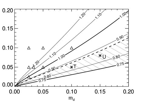
Figure 4: Contours of the disk stability parameter $\epsilon_{\rm m}$ (solid lines) for $c=15$. According to Syer, Mao & Mo Syer et al. (1998) disks with $\epsilon_{\rm m}\geq 0.75$ should be stable against bar formation, while the earlier work of Efstathiou, Lake & Negroponte Efstathiou et al. (1982) gives the condition $\epsilon_{\rm m}\geq 1.1$. Disk models lying below the thick dashed line are dominated by the disk gravity at the maximum of the disk rotation curve, thus the hatched region shows the parameter space that may contain stable disks which are not everywhere dominated by dark matter. Two of our models, ‘T’ and ‘U’ (stars), lie in this region. The other models are indicated as triangles.

Figure 5: Inner rotation curves of the models T, U, and V out to 5 disk scale lengths. The dashed line is the contribution of the disk, the dotted that of the dark halo, and the solid line gives the total rotation curve.

As the rotation curves in Fig. 1 show, all our ‘basic’ disk models A-F are gravitationally dominated by dark matter, even in the innermost regions of the disks. While the presence of a dark matter halo has been convincingly demonstrated by the flatness of observed rotation curves, there is still a controversy about the amount of dark matter in the inner regions of disk galaxies.

This controversy has arisen, because the decomposition of an observed rotation curve into a stellar and a dark matter component is rather ambiguous, since the result depends strongly on assumptions about the dark matter profile and the mass-to-light ratio (Navarro 1998). Traditionally, rotation curves have therefore been fitted using the ‘maximum-disk’ hypothesis, i.e. the largest mass possible is assigned to the disk consistent with the rotation curve. The recent work of Debattista & Sellwood (1998) suggests that the central density of dark matter in barred galaxies should be low, thus supporting the maximum-disk hypothesis. However, others (e.g. van der Kruit 1995) maintain that the contribution of dark matter in the inner regions of disk galaxies must be substantial. There is also recent observational work that supports this assertion (Quillen & Sarajedini 1997). We also note that even if the inner rotation curve of a galaxy can be well accounted for by a disk component alone, this does not provide evidence for the absence of dark matter in the inner parts of the disk.

The theoretical results employed in this work predict dark matter profiles with a central density cusp, and a resulting strong contribution of dark matter in the inner disks. We now briefly discuss, to what extent the model of MMW may also accommodate galaxies that are maximum-disk, or at least somewhat closer to it. In order to make the self-gravity of the disk more important, we can either reduce $\lambda$ (making the disk smaller), increase $m_{\rm d}$ (making the disk heavier), or lower $c$ (reducing the concentration of the halo). However, for fixed $m_{\rm d}$ and fixed $c$, disk-stability poses a lower limit on $\lambda$. Thin, fully self-gravitating disks have been known to be violently bar-unstable for a long time, a fact that suggested to Ostriker & Peebles (1973) that there must be dark matter that stabilizes the disks. Later, Efstathiou, Lake & Negroponte (1982) used N-body simulations to derive the stability criterion $\epsilon_{\rm m}\geq 1.1$ for the disk, where

$$\epsilon_{\rm m}\equiv\frac{v_{\rm max}}{(GM_{\rm d}/R_{\rm d})^{1/2}},$$ (40)

and $v_{\rm max}$ is the maximum rotation velocity. Recently, Syer, Mao & Mo (1998) confirmed that $\epsilon_{\rm m}$ is a good diagnostic for bar-instability, although they found a somewhat weaker stability criterion, $\epsilon_{\rm m}\geq 0.75$.

In Figure 4 we show contours of $\epsilon_{\rm m}$ in the $m_{\rm d}$-$\lambda$ plane. Also shown is the region, where the disk gravity at the maximum of the disk rotation curve is larger than the contribution by the dark matter. There is thus a small region of parameter space (hatched) where the galaxies are disk-dominated, but where they should be still stable against bar formation according to Syer et al. (1998). Incidentally, $\epsilon_{\rm m}\geq 1.0$ corresponds very closely to the condition $\lambda\geq m_{\rm d}$, the choice we employed so far.

Note that lowering $\lambda$ may not only render a disk unstable, it will also make it substantially smaller. Hence, the observed sizes of disk galaxies can also provide a lower bound on $\lambda$. Indeed, the results of MMW suggest that disks become too small if they lose a substantial part of their angular momentum to the dark halo. Since these arguments disfavour low $\lambda$, one may rather try to increase $m_{\rm d}$ to make the gravity of the disk more important. In principle, we expect that the universal cosmic baryon fraction poses an upper limit on $m_{\rm d}$, while the actual value of $m_{\rm d}$ could be a lot smaller if the efficiency of disk formation is low. Taking a big bang nucleosynthesis value of $\Omega_{\rm B}\simeq 0.015h^{-2}$ (Copi et al. 1995) for the baryon density, $m_{\rm d}$ should be smaller than 0.06 in a critical density universe with a Hubble constant of $h=0.5$. However, clusters of galaxies suggest that the baryon fraction is larger by at least a factor of three (White et al. 1993). Note that in a low density universe this can be reconciled with cosmic nucleosynthesis. If $\Omega_{0}$ is as low as 0.2, the limit on $m_{\rm d}$ goes up to about 0.15-0.2.

We examine these possibilities to a limited extent with three additional models which are disk-dominated in the inner regions. It is interesting to see how their tidal tails fit into the systematic properties of the other models. We label one of these models ‘T’, and give it the parameters $m_{\rm d}=0.1$, $\lambda=0.05$, $c=15$, $v_{200}=160\,\mbox{km s}^{-1}$, and $m_{\rm b}=0$. For a further model, called ‘U’, we instead adopt $m_{\rm d}=0.15$, $\lambda=0.08$, i.e. here we make the disk substantially more massive. Finally, we consider a model ‘V’ with a smaller concentration of the halo. Here we use $c=5$, $m_{\rm d}=0.1$, and $\lambda=0.05$. Hence this model is consistent with the value of $c\simeq 5$ favoured by Navarro (1998) in a recent analysis of a sample of spiral galaxies. Note that such low concentrations are theoretically expected for flat, low-density universes.

The inner rotation curves of these models are shown in Fig. 5. The stability parameter for them is $\epsilon_{\rm m}\simeq 0.84$. Hence they lie in the hatched region of Figure 4. In contrast to the other models, we here chose $\sigma_{R}=2.0\,\sigma_{z}$ for the velocity structure of the disk to prevent it developing a bar before the galaxies collide. This raises $Q$ to about 2.0, while it would have been $Q\simeq 1.0$ for our conventional choice for $\sigma_{R}$.

4.2 Collision simulations

The most favourable condition for making tidal tails are prograde encounters where the spin vectors of the disks are aligned with the orbital angular momentum. In this situation, the approximate resonance between the disk rotation and the orbital angular frequency amplifies the perturbation of particle orbits on the far sides of the disks, since they stay for a longer time in the region of the strongest tidal field.

Since we here try to achieve as prominent tails as possible, we usually set up our disk-disk collisions on prograde parabolic orbits. For simplicity we run only symmetric encounters between pairs of identical models; that is we collide model A with A, B with B, and so on.

We always chose the initial separation of the galaxies to be twice the virial radius. i.e. $R_{\rm start}=320\,h^{-1}{\rm kpc}$. The remaining undetermined orbital parameter is the orbital angular momentum. We specify it in terms of the minimum separation $R_{\rm kep}$ the galaxies would reach if they were point masses moving on the corresponding Keplerian orbit. In reality, once the galaxies overlap they will start to deviate from this trajectory due to dynamical friction. As a consequence, the actual separation $R_{\rm min}$ of the galaxies in their first encounter will generally be larger than $R_{\rm kep}$.

We examined three main choices for $R_{\rm kep}$, $3.5$, $7$ and $14\,h^{-1}{\rm kpc}$. For each of the models A, B, and C, we have run all three of these combinations, while we restricted ourselves to just one ‘impact parameter’ for the other models. Additionally, we simulated a set of wider encounters with $R_{\rm kep}=28$, 56, 112$\,h^{-1}{\rm kpc}$ for the C model. Runs labeled ‘A0’, ‘B0’, etc. refer to $R_{\rm kep}=3.5\,h^{-1}{\rm kpc}$, those containing the digits 1 or 2 to $7\,h^{-1}{\rm kpc}$ and $14\,h^{-1}{\rm kpc}$, respectively.

We also simulated two additional versions of run C2 where the disks do not have a prograde orientation. In the collision ‘C2r’ both disks are retrograde, i.e. their spins are just flipped, while in the model ‘C2i’ they are inclined by $90^{\rm o}$ relative to the orbital plane.

With respect to the bulge model and the disk-dominated models, we have only run one simulation in each case (‘W1’, ‘T1’, ‘U1’, ‘V1’), an encounter at $R_{\rm kep}=7\,h^{-1}{\rm kpc}$. Table 2 gives an overview of all these runs. Also shown in this table are the actual minimum separations $R_{\rm min}$ of the centers of the disks in their first encounter. We here defined the center of a disk as its densest point, and used a kernel interpolation like in smoothed particle hydrodynamics (SPH) to estimate the density of particles. However, using simply the center-of-mass of the indiviual disks gives similar results.

When the galaxies start to overlap, the interaction potential between them becomes shallower than that of the corresponding point masses. This effect will make the orbits wider than the Keplerian expectation. However, the galaxies are also slowed down by dynamical friction, an effect that brings the galaxies closer together. Both mechanisms compete with each other, and their relative strength depends on the distribution of mass inside the galaxy. As Table 2 shows, the minimum separations $R_{\rm min}$ are usually somewhat larger than the corresponding Keplerian value $R_{\rm kep}$. Note however, that the measurement of $R_{\rm min}$ has an uncertainty of order $\pm 1\,h^{-1}{\rm kpc}$, because we stored only a limited number of output times.

4.3 Numerical techniques

All the simulations in this work have been run with our GADGET-code (GAlaxies with Dark matter and Gas intEracT). It is a newly written SPH-code in C, specifically designed for the simulation of galaxy formation and interaction problems. The gravitational interaction is either computed with the special-purpose hardware GRAPE (if available) or with a TREE code. Time integration is performed with a multi-timelevel leapfrog integrator, with the thermal energy equation being integrated semi-implicitly. Time-critical routines (i.e. the force computation and neighbour search with the TREE or GRAPE) have been profiled and optimized extensively.

In this work, the SPH part of GADGET is not used; we just treat dark matter and stellar material as collisionless particles. Futher details of GADGET and an application of its SPH-capabilities will be described in future work.

For all of the basic models A to F, and for T to V, we used 20000 particles to represent each disk, and 30000 particles for each halo, hence each simulation had a total of $100000$ particles. We chose a gravitational softening length of $0.4\,h^{-1}{\rm kpc}$ for the dark matter, and $0.1\,h^{-1}{\rm kpc}$ for the disk. Time integration was performed with high enough accuracy, such that the total energy was conserved to better than $0.8\%$ in all runs.

For the bulge model W, we used an additional 10000 particles for each bulge, and we employed a softening of $0.1\,h^{-1}{\rm kpc}$ for the bulge as well.

Some of the models have been integrated using GRAPE (A0, B0, B2, E2, F2, T1, U1, W1), the others with the TREE code. For the latter we used the cell opening criterion of Dubinski (1996) with $\theta=1.0$, we included quadrupole moments, and we matched the spline softening of the TREE code to the Plummer softening of GRAPE cited above.

Each simulation was run for 2.6 internal time units, or 0.26 Hubble times, corresponding to $2.54\times 10^{9}\,h^{-1}\mbox{yr}$. At this point of time, the merger remnants are not yet fully relaxed, but the tidal tails have already largely decayed.

5 Results

5.1 Dynamical evolution of the models

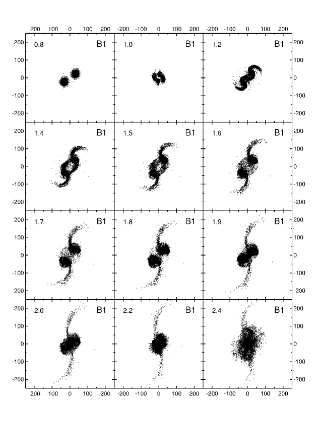
Figure 6: Time evolution of run B1. The panels show the disk particles projected onto the orbital plane. The length units labeling the axes are given in $\,h^{-1}{\rm kpc}$. The elapsed time since the start of the simulation (upper left corners) is given in units of 0.1 Hubble times, or $9.8\times 10^{8}\,h^{-1}{\rm yr}$.

Figure 6 shows a representative example of the time evolution of one of our runs (B1). Overall, the models follow the well-known behaviour of close encounters of pairs of disk galaxies. When the galaxies reach orbital centre, violent tidal forces induce a bar instability that quickly transforms the disks into a pair of open bisymmetric spirals. Simultaneously, disk material from the far side of the encounter is ejected by the tidal field into arcing trajectories that later form tidal arms. Material from the near side is drawn towards the companion, giving rise to bridges between the galaxies as they temporarily separate again. While the bridges are destroyed when the galaxies come back together for a second time, the tails can survive and grow for a longer time in the relatively quiet regions of the outer potential.

Nevertheless, the dynamical evolution of the tidal tails is quite rapid. After their initial phase of expansion, the most strongly bound material in the inner region of the tail quickly starts to rain back onto the merging pair. Eventually, this also happens to material progressively further out, such that the surface density and prominence of the tidal tails quickly decrease with time.

Figure 7: Comparison of tidal tails between different runs. All the panels show the disk particles projected onto the orbital plane at the same time since the start of the simulation. The top 9 panels display runs that involve the disk models A-C for the set of impact parameters $R_{\rm kep}=3.5$, 7, and 14$\,h^{-1}{\rm kpc}$ (indicated by the digits 0, 1, and 2, respectively, in the labels of the runs). From A to C, the spin parameter $\lambda$ increases in the sequence 0.025, 0.05, and 0.1, but all three models have an equal disk mass given by $m_{\rm d}=0.025$. In the lower three panels we show additional collisons of model C with wider impact parameters in the sequence $R_{\rm kep}=28$, 56, and 112$\,h^{-1}{\rm kpc}$.

Figure 8: Comparison of tidal tails between different runs. The panels show the disk particles projected onto the orbital plane at the same time since the start of the simulation. Runs D1 and E2 involve models with twice as heavy disks ($m_{\rm d}=0.05$) than A-C, while F2 has $m_{\rm d}=0.1$. The D-model has a spin parameter of $\lambda=0.05$, while the E- and F-disks have $\lambda=0.1$. The T ($m_{\rm d}=0.1$, $\lambda=0.05$) and U ($m_{\rm d}=0.15$, $\lambda=0.08$) models are disk-dominated in their inner regions, while model W ($m_{\rm d}=0.034$, $m_{\rm b}=0.016$ $\lambda=0.05$) also contains a bulge. The digit in the label of the runs parameterizes the impact parameter; 0, 1, and 2 are for $R_{\rm kep}=3.5$, 7, or 14$\,h^{-1}{\rm kpc}$, respectively.

5.2 Comparison of tidal tails

Depending on the strength of the tidal response, the tidal tails can contain a varying amount of mass, and reach different lengths. By comparing the time evolution of the models A to C, such differences are readily apparent. For example, the tails of the larger disks of run C1 are much more massive and prominent than those of run B1, while the tails of the small disks of simulation A1 are rather thin and anemic. However, the spatial extent of the tails is quite comparable in the models. When normalized to the initial disk scale length the anemic tails of the A-models are even longer than those of the C-models.

These trends are clearly visible in Figures 7 and 8, where we compare different runs at the same time, approximately corresponding to the moment when the tails are most impressive. Note however, that due to the rapid evolution of the morphology of the tidal tails it is not easy to compare different models at exactly equivalent times of dynamical evolution.

When models with different impact parameters are compared, some finer trends in the tail morphology may be observed. With growing impact parameter (labels $0\to 2$), the bridges between the galaxies become more pronounced, and the tails are slightly more curved. This is related to the larger orbital angular momentum of these encounters.

Note that the runs A, B, and C of Figure 7 all have a large halo-to-disk mass ratio of more than 40:1, i.e. according to DMH none of these models should have produced prominent tails. Nevertheless, the spatial extent of the tails is often quite large. For example, the B-models with a disk scale length of $R_{\rm d}\approx 3.5\,h^{-1}{\rm kpc}$ produce tails reaching $200\,h^{-1}{\rm kpc}$ in length, i.e. about 60 times the original disk scale length.

When tails of models with different halo-to-disk mass ratio but equal spin parameter are compared, it becomes clear that the mass ratio cannot be the relevant parameter that decides whether tails form or not. For example, the tails of runs E2 and F2 in Figure 7 may be compared to the ones of run C2. Despite a variation of the mass ratio by a factor 4 or so, the tails are almost equally strong in these three simulations. This is clearly due to the approximately equal size of the disks in these models. Because the dark matter is gravitationally dominant even in the regions of the disks, the disk stars behave almost like test particles in the gravitational potential of the dark halo. In this limiting case it is clear, that only the location of the disk material inside the dark halo determines the disk response, i.e. it is the relative size of disk and dark halo that matters.

5.3 An indicator for tidal response

As we have seen above, knowledge of the halo-to-disk mass ratio is by no means sufficient to predict how prone a particular galaxy model is to tail formation. MMW suggested using the quantity

$${\cal E}=\left[\frac{v_{\rm e}(R)}{v_{\rm c}(R)}\right]^{2}$$ (41)

as a more suitable indicator. ${\cal E}$ compares the depth of the potential well with the specific kinetic energy of the disk material. The quantity ${\cal E}$ also arises, when one tries to estimate the relative increase $\Delta E$ of specific kinetic energy of disk stars in a nearly head-on encounter of identical disk models. In this situation one finds (Binney & Tremaine 1987; Mo, Mao & White 1998)

$$\Delta E/v_{\rm c}^{2}\simeq\left(\frac{v_{\rm c}}{v_{\rm e}}\right)^{2}=1/{\cal E}.$$ (42)

This suggests the use of ${\cal E}$ as an indicator for the susceptibility of a disk model to tidal perturbations. In order to obtain a typical value for ${\cal E}$ we evaluate it at $R=2R_{\rm d}$, which is about the half mass radius of the disk.

Figure 9: Tidal response $T$ as a function of time for three selected runs. We define $T$ as the mass fraction of each disk that reaches a distance of more than $10R_{\rm d}$ to its center-of-mass. Also indicated as horizontal lines are the values of $T_{\rm eff}$ that we take as measure for the tidal response of the disk. Since we only stored simulation outputs with a spacing of $0.1$ time units, the measurement of $T_{\rm eff}$ is slightly uncertain.

Figure 10: Tidal response $T_{\rm eff}$ of the different runs versus the value of ${\cal E}$ for the corresponding disk model, where ${\cal E}$ is evaluated at $R=2R_{\rm d}$. The measurement of $T_{\rm eff}$ is slightly uncertain, and $T_{\rm eff}$ also depends on details of the orbital parameters of the encounter. However, our runs are designed to produce very nearly the strongest tails possible for a given disk model. At fixed ${\cal E}$, it should therefore be hard to find a model that gives a higher value for $T_{\rm eff}$ than the maximum of our runs. In other words, there should be no model in the region above the indicated dashed line.

Figure 11: Tidal response $T_{\rm eff}$ of the different runs versus the disk-to-halo mass ratio (left panel), and versus $M(2R_{\rm d})/M$ (right panel). The quantity $M(2R_{\rm d})/M$ is a measure of the fraction of the total mass in the disk region.

We now want to test how well ${\cal E}$ works as an indicator for the ability of a particular disk-halo model to develop massive tails. Here one encounters two immediate problems.

First, the tidal response of a disk depends on the orbital parameters of the encounter with its companion. For example, if a disk is tilted against the orbital plane, the tidal forces felt by the bulk of the disk material will generally be smaller, resulting in a less prominent tidal tail. Similarly, a change of the impact parameter or the orbital energy can affect the tidal response. We here do not intend to investigate the complete parameter space. Rather, we focus on collisions that produce the strongest tails possible for mergers of a given disk model.

Figure 12: Tidal tails of simulations C2r and C2i. The panels show the disk particles, projected either onto the xy-plane (orbital plane), or the yz-plane. Apart from a different orientation of the disks, runs C2r and C2i are identical to C2. In C2r, both disks are retrograde, while in C2i the spins of the disks lie in the orbital plane, pointing along the x-axis. These runs may be compared with C2 shown in Figure 7.

In this spirit, prograde encounters are an obvious choice for the orientations of the disks, since this configuration has repeatedly been shown to produce the strongest tails, and we here confirm this with the runs C2r and C2i. We use parabolic orbits, because they are plausible candidates for real interacting galaxies if one assumes that they are coming together for their first time. However, even when this assumption is dropped, DMH showed that moderately bound orbits are no more effective in producing tails than zero energy orbits. With respect to the ‘impact’ parameter $R_{\rm kep}$, we have examined a range of different choices and found that the tails appear to be of maximum strength for $R_{\rm min}\approx 2-6R_{\rm d}$, i.e. in collisions where the disks pass each other at a distance of a few disk scale lengths. Hence, our merger simulations of equal disk galaxies have been set up to exhibit the most favourable conditions for tail formation, and should indeed produce the strongest tails possible for these disk models.

Second, it is not obvious how to define the mass or extent of the tidal tails in an objective way. This is further complicated by the rapid dynamical evolution of the tails, which makes it difficult to compare simulations that may form their tails at different times.

In order to solve this problem and measure the strength of the tidal response, we have come up with the following scheme. We start by defining the quantity $T$ to be the mass fraction of each disk that reaches a distance of more than $10R_{\rm d}$ from its center-of-mass, where $R_{\rm d}$ is the original scale length of the unperturbed disk.

In Figure 9 we show examples for the time evolution of $T$. Shortly after the disks come together for the first time, $T$ jumps up, reaches a maximum, and slowly decays, until the disks are scrambled up in their second encounter and $T$ loses its initial meaning. Note that the different runs reach their maximum of $T$ at different times. In order to compare them on an equal footing, we therefore define an effective response $T_{\rm eff}$ as the peak value reached by $T$.

In Figure 10 we plot the tidal response $T_{\rm eff}$ of our runs versus the value of ${\cal E}$, evaluated at $R=2R_{\rm d}$. Although our coverage of parameter space is limited, it is nevertheless clear that there is a correlation between $T_{\rm eff}$ and ${\cal E}$. Of course, there is some uncertainty in the measurement of $T_{\rm eff}$ and this introduces some scatter. Also, for fixed ${\cal E}$, the tidal response $T_{\rm eff}$ depends somewhat on the impact parameter $R_{\rm kep}$, and it might also have a slight dependence on $m_{\rm d}$. However, to the extent that our simulations really produce the strongest tails possible for our disk models, Fig. 10 shows that it will be exceedingly hard to find a model that produces tails that lie above the dashed diagonal line. This establishes that ${\cal E}$ is a good indicator for the maximum tidal response $T_{\rm eff}$, that may be obtained for a given class of disk models. In particular, models with ${\cal E}\geq 8$ should be unable to produce strong tails. This is in excellent agreement with the analysis of MMW, who estimated ${\cal E}=4.2$, 5.5, 7.2, and 9.3 (in order of increasing halo mass) for the sequence of four models of DMH; in agreement with Figure 10, the last two of these models failed to produce prominent tails.

Figure 10 may also be compared to the two panels of Figure 11. In the left panel, we plot the tidal response versus the disk-to-halo mass ratio. This again shows, that the disk-to-halo mass ratio is not a good indicator for the ability to form tidal tails. For example, the models A, B, and C differ subtantially in the mass of their tails despite their equal disk-to-halo mass ratio. However, if we use instead the ratio of the total amount of mass in the region of the disk to the total mass of the galaxy, the mass ratio criterion can be partly resurrected. This is shown in the right panel of Fig. 11, where we plot $T_{\rm eff}$ versus $M(2R_{\rm d})/M$. Here $M(2R_{\rm d})$ is the total mass inside two disk scale lengths, and $M$ is the total mass of the galaxy and its halo. In this formulation, the mass ratio measures the relative distribution of mass within the system, and is a fair indicator of the ability of a galaxy model to form tidal tails. However, a detailed comparison with Fig. 10 shows, that ${\cal E}$ does a better job than $M(2R_{\rm d})/M$. For example, the model T1 appears as an outlyer in Fig. 11, failing to fit the monotonic trend of larger $T_{\rm eff}$ with increasing $M(2R_{\rm d})/M$, but fits within the general distribution in Fig.  10.

Starting from a head on collision, Figure 10 also shows that the tidal response $T_{\rm eff}$ becomes larger as the impact parameter $R_{\rm kep}$ is increased. However, for very wide encounters one expects only a small distortion of the disks. As the sequence of models C0-C5 demonstrates, there is indeed a maximum response for an intermediate impact parameter $R_{\rm kep}$ of order a few disk scale lengths.

Also, the orientation of the disks is an important factor in determining the strength of the disk response. In the retrograde collision C2r, the spins of the galaxies are just reversed compared to C2, yet this already makes the tidal tails much weaker, as seen in Figure 12. Similarly, the inclined galaxies of simulation C2i produce tails that are less extended than those of run C2.

We also note that the simulations T1, U1, and V1, in which our ‘disk-dominated’ models collide, produce tidal tails well in line with the general trend of Figure 10.

5.4 A model with a bulge

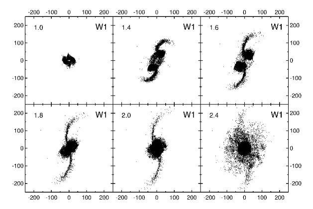
Figure 13: Time evolution of run W1, which collides our disk+bulge model with itself. The top series of panels displays the disk particles projected onto the orbital plane, while the bottom panels show the bulge particles. The length units refer to $\,h^{-1}{\rm kpc}$, and the elapsed time since the start of the simulation (upper left corners) is given in units of 0.1 Hubble times, or $9.8\times 10^{8}\,h^{-1}{\rm yr}$.

In Figure 13 we show the time evolution of run W1, which collides two disk$\,+\,$bulge galaxies. These disk galaxies (our model W) are descendents of model D, but one third of the stellar mass has been put into a centrally concentrated bulge. This results in a rotation curve (Figure 3) that is practically flat up to the very center of the disk, with a shape quite similar to the models of DMH.

Due to their strong central concentration, the bulges survive largely unaffected until their final coalescence. However, the disks develop prominent tails that appear to be similar in strength to the other models with specific angular momentum corresponding to $\lambda=0.05$. A measurement of $T_{\rm eff}$ shows that the strength of the tails is in fact quite similar to the directly comparable simulation D1. Also, the run W1 fits well into the plot of Figure 10, although the inner structure of model W is very different from that of the other models.

This suggests that bulges are not effective in preventing tail formation, at least as long as they primarily affect the inner rotation curve.

6 Discussion

In this study we constructed N-body models of disk galaxies with structural properties directly motivated by current theories of hierarchical galaxy formation. In particular, the mass of the dark haloes in these models is much larger than that of the stellar disks. In the most extreme models we consider, the halo-to-disk mass ratio is larger than 40:1.

Provided the spin parameter is not too small, these models can produce long and massive tidal tails, despite the massive haloes. Halo-to-disk mass ratio is not a useful indicator for tail-making ability.

Instead, the size of the disk compared to that of the halo seems to be the critical factor. In our approach, the size of the disk is tied to the spin of the dark halo. A larger spin parameter $\lambda$ leads to larger disks. The bulk of the disk material is then more loosely bound in the dark matter potential well and can be more easily induced to form long tidal tails. This effect can be quantified in terms of the ratio ${\cal E}$ of the circular velocity to the escape speed at a radius $R=2R_{\rm d}$. We have shown that ${\cal E}$ correlates well with the tidal response of the disk models. For models with ${\cal E}\geq 8$ we do not expect significant tails, while models with ${\cal E}\leq 6.5$ can produce substantial tails.

When ${\cal E}$ is used to characterize the tail-making ability, the results of DMH agree with our own. In their sequence of four models not only the mass of the halo changes, but also its spatial extent. We think the latter effect is critical in defining tail-making ability, because the relative size of disk and halo affects the value of ${\cal E}$ strongly. This also agrees with the earlier conclusion of Barnes (1997, private communication). For given inner structure and given mass ratio $M_{\rm d}/M_{\rm h}$, less extensive halos have larger ${\cal E}$ and so make weaker tails.

We focused in this work on just one halo mass. Note however, that the shape of the rotation curves does not depend on our particular choice for $v_{200}$. Rotation curves with other peak velocities may be realized by an appropriate scaling of $v_{200}$.

According to the work of NFW, the shape of the dark matter profile is insensitive to cosmology. Also, the distribution of $\lambda$ is universal and independent of the initial power spectrum. Furthermore, the average value of the concentration $c$ does not vary with halo mass, and it depends only weakly on cosmology. For low-density flat universes a smaller value, $c\simeq 5$, is probably more appropriate than the value $c=15$ employed in most of the models in this work. Such a smaller concentration is also supported by observational data (Navarro 1998). However, our model ‘V1’, which has $c=5$, produces tails well in line with the other models in Figure 10. Also note that according to Figure 2, smaller $c$ gives rise to larger disks, in principle favouring even stronger tails.

This suggests that all ‘reasonable’ CDM cosmologies can produce disk galaxies with $\lambda\geq 0.05$ that are roughly equally capable of producing tidal tails when they collide and merge with similar objects. We conclude that the observed lengths of tidal tails in interacting galaxies are consistent with current CDM cosmologies, and that tidal tails are not useful to discriminate between different flavours of these scenarios.

We hope that the N-body representations of disk models constructed in this work may be more realistic caricatures of real spiral galaxies than those of previous work. In particular, the structural properties of our models are motivated by hierarchical structure formation and are less ad hoc than in previous simulations of this kind. These models should be useful for future work on galaxy evolution.

References

- Barnes (1988) Barnes J. E., 1988, ApJ, 331, 699
- Barnes (1989) Barnes J. E., 1989, Nature, 338, 123
- Barnes (1992) Barnes J. E., 1992, ApJ, 393, 484
- Barnes & Hernquist (1996) Barnes J. E., Hernquist L., 1996, ApJ, 471, 115
- Binney & Tremaine (1987) Binney J., Tremaine S., 1987, Galactic Dynamics, Princeton University Press
- Colina et al. (1991) Colina L., Lipari S., Macchetto F., 1991, ApJ, 379, 113
- Copi et al. (1995) Copi C. J., Schramm D. N., Turner M. S., 1995, Science, 267, 192
- Debattista & Sellwood (1998) Debattista V. P., Sellwood J. A., 1998, ApJ, 493, L5
- Dubinski (1996) Dubinski J., 1996, New Astronomy, 1, 133
- Dubinski et al. (1997) Dubinski J., Hernquist L., Mihos J. C., 1997, preprint, astro-ph/9712110
- Dubinski et al. (1996) Dubinski J., Mihos J. C., Hernquist L., 1996, ApJ, 462, 576
- Efstathiou et al. (1982) Efstathiou G., Lake G., Negroponte J., 1982, MNRAS, 199, 1069
- Farouki & Shapiro (1982) Farouki R. T., Shapiro S. L., 1982, ApJ, 259, 103
- Farouki et al. (1983) Farouki R. T., Shapiro S. L., Duncan M. J., 1983, ApJ, 265, 597
- Hernquist (1992) Hernquist L., 1992, ApJ, 400, 460
- Hernquist (1993a) Hernquist L., 1993a, ApJS, 86, 389
- Hernquist (1993b) Hernquist L., 1993b, ApJ, 409, 548
- Hibbard & Mihos (1995) Hibbard J. E., Mihos J. C., 1995, AJ, 110, 140
- Lemson & Kauffmann (1998) Lemson G., Kauffmann G., 1998, preprint, astro-ph/9710125
- Magorrian & Binney (1994) Magorrian J., Binney J., 1994, MNRAS, 271, 949
- Mihos & Bothun (1997) Mihos J. C., Bothun G. D., 1997, ApJ, 481, 741
- Mihos et al. (1998) Mihos J. C., Dubinski J., Hernquist L., 1998, ApJ, 494, 183
- Mo et al. (1998) Mo H. J., Mao S., White S. D. M., 1998, MNRAS, 295, 319
- Navarro (1998) Navarro J. F., 1998, preprint, astro-ph/9807084
- Navarro et al. (1996) Navarro J. F., Frenk C. S., White S. D. M., 1996, ApJ, 462, 563
- Navarro et al. (1997) Navarro J. F., Frenk C. S., White S. D. M., 1997, ApJ, 490, 493
- Navarro & Steinmetz (1997) Navarro J. F., Steinmetz M., 1997, ApJ, 478, 13
- Navarro & White (1994) Navarro J. F., White S. D. M., 1994, MNRAS, 267, 401
- Negroponte & White (1983) Negroponte J., White S. D. M., 1983, MNRAS, 205, 1009
- Ostriker & Peebles (1973) Ostriker J. P., Peebles P. J. E., 1973, ApJ, 186, 467
- Quillen & Sarajedini (1997) Quillen A. C., Sarajedini V. L., 1997, preprint, astro-ph/9705192
- Syer et al. (1998) Syer D., Mao S., Mo H., 1998, preprint, astro-ph/9711160
- Toomre & Toomre (1972) Toomre A., Toomre J., 1972, ApJ, 178, 623
- van der Kruit (1995) van der Kruit P. C., 1995, in Stellar Populations, edited by P. C. van der Kruit, G. Gilmore, 205, in IAU Symp. 164, Kluwer
- Warren et al. (1992) Warren M. S., Quinn P. J., Salmon J. K., Zurek W. H., 1992, ApJ, 399, 405
- Weil et al. (1998) Weil M. L., Eke V. R., Efstathiou G., 1998, preprint, astro-ph/9802311
- White (1978) White S. D. M., 1978, MNRAS, 184, 185
- White (1979) White S. D. M., 1979, MNRAS, 189, 831
- White et al. (1993) White S. D. M., Navarro J., Evrard A. E., Frenk C. S., 1993, Nature, 366, 429