The use of Minimal Spanning Tree to characterize the 2D cluster galaxy distribution

Abstract

We use the Minimal Spanning Tree to characterize the aggregation level of given sets of points. We test 3 distances based on the histogram of the MST edges to discriminate between the distributions. We calibrate the method by using artificial sets following Poisson, King or NFW distributions. The distance using the mean, the dispersion and the skewness of the histogram of MST edges provides the more efficient results. We apply this distance to a subsample of the ENACS clusters and we show that the bright galaxies are significantly more aggregated than the faint ones. The contamination provided by uniformly distributed field galaxies is neglectible. On the other hand, we show that the presence of clustered groups on the same cluster line of sight masked the variation of the distance with the considered magnitude.

1 Introduction

Clusters of galaxies are the largest (partially) virialized structures in the Universe and the cosmological parameters may have a strong influence on their profile. The determination of the cluster density profile shape is a crucial question. A high value of $\Omega$ gives for example steeper asymptotic profiles in the simulations (i.e. Crone et al 1994, Jing et al. 1995). It is then possible to recover the value of $\Omega$ with the shape of the clusters. We note however that other studies (see Navarro et al. 1995, 1996) argue that the dark matter profiles in clusters deduced from the CDM model are identical whatever the details of the model.

Similarly, it is important to know if the cluster profiles exhibit a cusp (e.g. Adami et al. 1998). After an analyze of a subsample of the ENACS clusters, Adami et al (1998) conclude that clusters have a core if we consider the galaxies brighter than b_j = 20. The ENACS clusters (e.g. Katgert et al. 1996 or Mazure et al. 1996) obey the model of a relaxed system (e.g. King 1962). However, the bright galaxies (B${}_{j}\leq$-18.5) are equally fitted by a profile with core or with cusp. It is then crucial to know how the shape of the galaxy distribution vary with the magnitude of the tested galaxies. Adami et al. (1998) have fitted different profiles with different shape for the considered magnitudes. This method is very efficient and quantitative but also time consuming and complex according to the large number of parameters.

We develop here a new way to characterize the variation with magnitude of the aggregation of the galaxies in clusters, without any profile fitting. We use the Minimal Spanning Tree (or MST hereafter) which is common in astronomy to the study of the very large scale structures (e.g. Barrow et al. 1985, Bhavsar & Splinter 1996 or Krzewina & Saslaw 1996). It is also used in physic to study order and disorder of a given set of points (e.g. Dussert et al. 1986). We use here this last aspect to study the density profiles of clusters of galaxies by using only a bidimensionnal analysis. The first part of the article is about the MST theory and the calibration of the method. We apply the method in the second part to a subsample of 15 very rich and very regular clusters in order to calibrate the method. The last part is our conclusions.

We use H₀=100 km.Mpc^-1.s^-1 and q₀=0.

2 The MST: theory and calibration

2.1 theory

The MST is a geometrical construction issued from the graph theory: the used definitions are given in Dussert (1988). Very briefly, it is a tree joining all the points of a given set, without a loop and with a minimal length; each point is visited by the tree only 1 time. The main aspect here is the unicity of such a construction. For a given set of points, there are more than 1 MST, but the histogram H of the MST edges is unique. This is fundamental because it is then possible to completely characterize a set of points with H.

Traditionally, only the two first momenta of H mean m and dispersion $\sigma$ are used. These two parameters are efficient for a gaussian distribution. To characterize some non gaussian distributions, we have to use more advanced momenta like the skewness s and/or the curtosis c. We have tested the use of these parameters in the following. Below, we describe the methodology:

• The Prim algorithm (1957) is used to construct the MST and compute the histogram H of edges.

• A point is chosen at random in the set and is the first MST element.

• A point which is the nearest of the MST point, is joined to the MST and removed from the set. The first MST edge is between these two points.

• We look for the set point which is the nearest of the MST points, join it to the MST and remove it from the set. The next MST edge is between this point and its nearest MST point.

• We repeat the operation for all the other set points.

This algorithm is designed to be the fastest one to have a MST on a given set of points. We normalize the lengths of the MST by using the Beardwood et al. (1959) study. A good approximation of the total length of a MST constructed with a random set of N points in an area S is $\frac{\sqrt{S\times N}}{N-1}$. So, we divide all the length by this factor (where S is the area of the maximum rectangle of the point set). We calculate finally the mean m, the dispersion $\sigma$, the skewness s and the curtosis c of H.

2.2 Calibrations of the method

We test our algorithm using simulations. We calculate m,$\sigma$,s,c for different sets of simulated points. The points are generated in a 500$\times$500 boxes. We note here that we normalize the distances and so, the unity of the box size is not important.

In order to characterize the cuspiness degree of the distributions, we use three kind of 2D density profiles: points randomly distributed (Poisson distribution), distributed with a centered King profile (flat profile in the center) and distributed with a centered NFW profile (cusped profile in the center: Navarro et al. 1995). We note here that the NFW expression was for a 3D distribution. Applying it for a 2D set of points generate a more cusped profile compare to the original 3D NFW. However, we will speak of ”NFW profiles” hereafter. The way we generated sets of points with a given profile is described in Adami (1998) and is related to the techniques described in Press et al. (1992). If $\rho$ is the density and r the radius, we have:

$$\rho_{2D\_King}(r)=\frac{1}{1+(\frac{r}{r_{c}})^{2}}$$

and

$$\rho_{2D\_NFW}(r)=(\frac{1}{\frac{r}{r_{c}}(1+\frac{r}{r_{c}})^{2}})^{2/3}$$

We will call hereafter r_c the characteristic radius of a given profile. For the King profile, it is the core radius and for the NFW profile it is a characteristic radius (no core for this profile). We simulate 8 sets of random distributions: with 10, 25, 60, 125, 250, 500, 750 and 1000 points.

For each set of points with a given profile and a given size, we proceed 100 realizations and so 100 calculations of m,$\sigma$,s,c. From these data, we are able to compute the mean value and the dispersion of each parameter m, $\sigma$ ,s or c.

2.2.1 Poisson distributions

We plot in figure 1 (m,$\sigma$) and (s,c) for a Poisson distribution.

Figure 1: Variation with the size N of the sample of: up: (m,$\sigma$), m is the upper line and $\sigma$ is the lower line and down: (s,c), s is the line with error bars and c is the line without error bar.

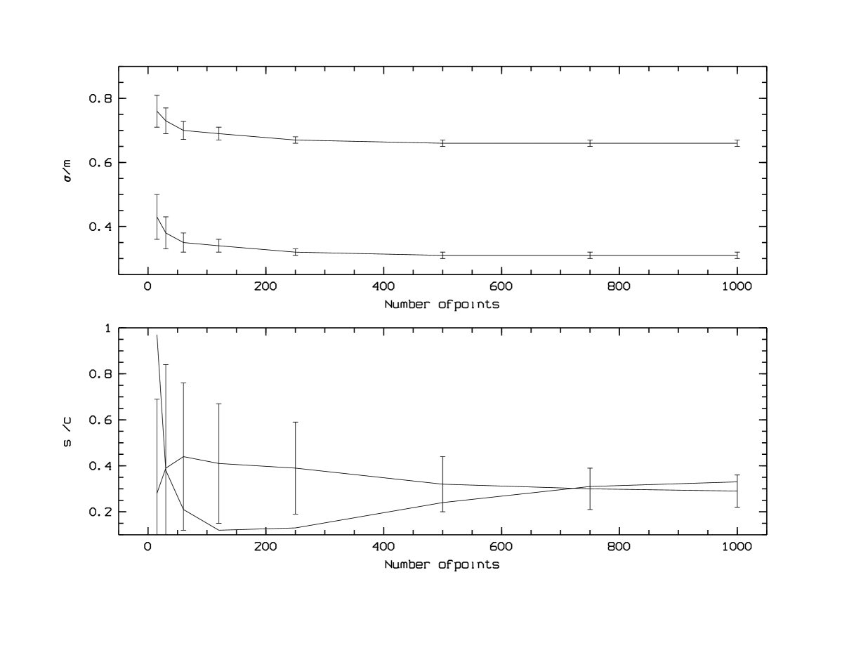
The parameters m and $\sigma$ are asymptotically equal to 0.66$\pm$0.02 and 0.31$\pm$0.02 in perfect agreement with Dussert (1988). The error bars are 3% of the mean value. The final value is reached for a number N of points in the simulation greater than 125.

The skewness s is well defined for N$\geq$250 with a final value of 0.29$\pm$0.14. The errors are greater: about 50% of the mean value.

The curtosis c is well defined only for N$\geq$750 with very large error bars ($\sim$100 % of the mean value). The final value is 0.33.

2.2.2 King and NFW profiles

Figure 2: Variation with the characteristic radius of the King distribution of: upper left: (m,$\sigma$) and 250 points (the increasing line is m and the decreasing line is $\sigma$), upper right: (s,c) and 250 points (s is the line with error bars and c is the line without error bar), lower left: (m,$\sigma$) and 500 points (the increasing line is m and the decreasing line is $\sigma$), lower right: (s,c) and 500 points (s is the line with error bars and c is the line without error bar).

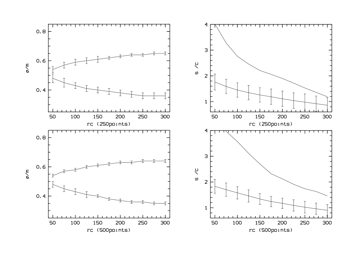
We calculate (m,$\sigma$,s,c) for different characteristic radii r_c of King and NFW profiles. We use r_c=50, 75, 100, 125, 150, 175, 200, 225, 250, 275 and 300 kpc. For a given profile and a given characteristic radius, we simulate 2 sets of points: 250 and 500. We plot the variation of (m,$\sigma$) and (s,c) with r_c for these 2 sets of points in figure 2 for the King profiles. The parameters vary significantly with r_c at the 3 $\sigma$ level. The size of the errors are similar to those for the Poisson case: very small for (m,$\sigma$), median for s and very large for c. The parameters (m,$\sigma$) are not significantly different from the Poisson case for large characteristic radii ($\geq$225 kpc). The skewness is significantly different at the 1 $\sigma$ level from the Poisson case whatever the characteristic radius. The mean value of the curtosis is also different, but not significantly because of the large error bars.

Figure 3: Variation with the characteristic radius of the NFW distribution of: upper left: (m,$\sigma$) and 250 points (the increasing line is m and the decreasing line is $\sigma$), upper right: (s,c) and 250 points (s is the line with error bars and c is the line without error bar), lower left: (m,$\sigma$) and 500 points (the increasing line is m and the decreasing line is $\sigma$), lower right: (s,c) and 500 points (s is the line with error bars and c is the line without error bar).

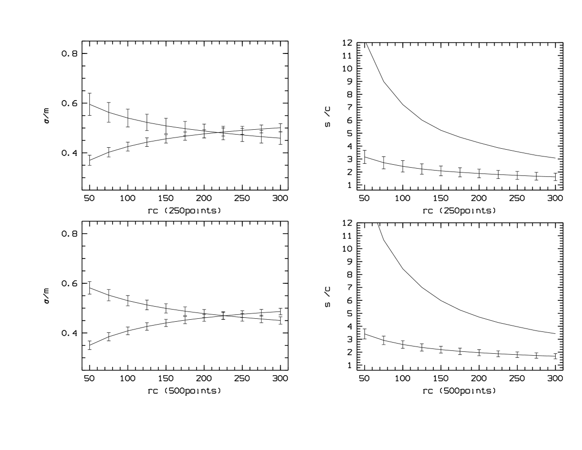
In figure 3 we plot the variations for the NFW profiles and the trends are very different. All the parameters (m,$\sigma$,s,c) differ significantly at the 1 $\sigma$ level from the Poisson case. We also notice an important degeneracy between m and $\sigma$.

2.2.3 Discrimination between the 3 profiles

We want to determine a parameter based on m, $\sigma$, s and c which is able to discriminate the three profiles. We want to test the distance in a n dimensional space with n=2, if we use (m,$\sigma$), n=3 if we use (m,$\sigma$,s) and n=4 if we use (m,$\sigma$,s,c). More generally, the distance in a space of n dimensions between (p₁, p₂, ….., p_n) and (q₁, q₂, ….., q_n) is

$$\Delta=\sqrt{\sum_{i=1}^{n}(p_{i}-q_{i})^{2}}$$

The error on a such distance is calculated by derivation:

$$d\Delta=\frac{\sum_{i=1}^{n}(p_{i}-q_{i})(dp_{i}+dq_{i})}{\Delta}$$

where $dp_{i}$ and $dq_{i}$ are the errors on $p_{i}$ and $q_{i}$.

Therefore, we define three distances: $\Delta_{m,\sigma}$, $\Delta_{m,\sigma,s}$, and $\Delta_{m,\sigma,s,c}$.

We calculate these distances for the Poisson distribution and the King and the NFW profiles for 3 different sets of points (50, 125 and 500) and for all characteristic radii. We plot (with errors) in figures 4, 5 and 6 these distances as a variation of the characteristic radius. We symbolize the nul distance as a solid line and we plot the error on the determination of the parameters of the Poisson distributions.

Figure 4: Variation with the characteristic radius of the 3 tested distances between the Poisson and the King distribution (crosses) and the Poisson and the NFW distribution (circles). We have 50 points in the samples. We plot the error bar on each points and we symbolize the error on the parameters of the Poisson distribution with the two horizontal dashed lines. The horizontal solid line symbolizes the nul distance to the Poisson distribution. The left part of the figure is for the distance $\Delta_{m,\sigma}$, the lower right part is for $\Delta_{m,\sigma,s}$ and the upper right part is for $\Delta_{m,\sigma,s,c}$.

Figure 5: Variation with the characteristic radius of the 3 tested distances between the Poisson and the King distribution (crosses) and the Poisson and the NFW distribution (circles). We have 125 points in the samples. We plot the error bar on each points and we symbolize the error on the parameters of the Poisson distribution with the two horizontal dashed lines. The horizontal solid line symbolizes the nul distance to the Poisson distribution. The left part of the figure is for the distance $\Delta_{m,\sigma}$, the lower right part is for $\Delta_{m,\sigma,s}$ and the upper right part is for $\Delta_{m,\sigma,s,c}$.

Figure 6: Variation with the characteristic radius of the 3 tested distances between the Poisson and the King distribution (crosses) and the Poisson and the NFW distribution (circles). We have 500 points in the samples. We plot the error bar on each points and we symbolize the error on the parameters of the Poisson distribution with the two horizontal dashed lines. The horizontal solid line symbolizes the nul distance to the Poisson distribution. The left part of the figure is for the distance $\Delta_{m,\sigma}$, the lower right part is for $\Delta_{m,\sigma,s}$ and the upper right part is for $\Delta_{m,\sigma,s,c}$.

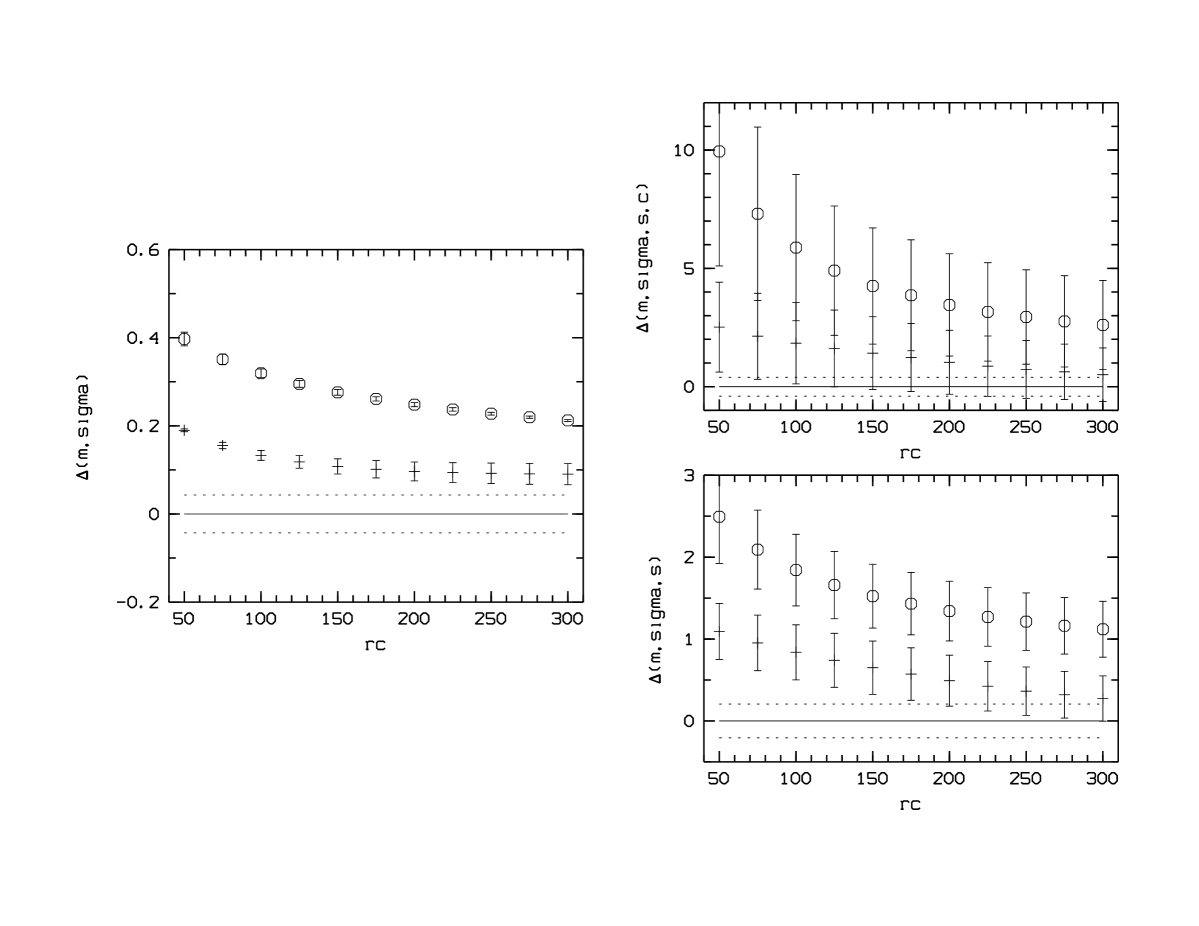
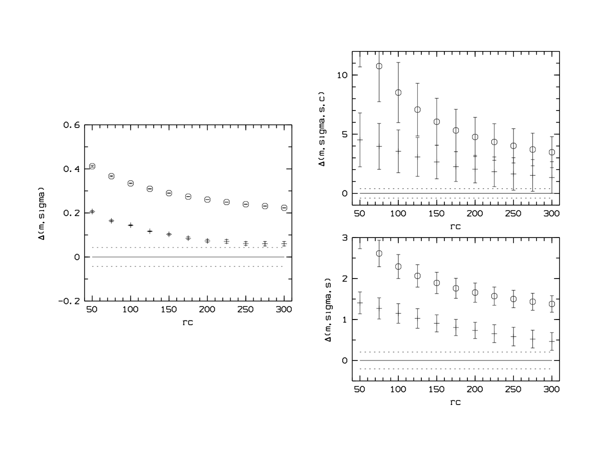
From these figures, we notice the following:

• First of all, the difference between the Poisson distribution and King and NFW profiles increases with the number of points.

• For 50 points, we have much confusion between the King and NFW profiles, as well as with the Poisson distribution whatever the distance used. It is impossible to characterize the distributions of 50 points.

• For 125 or 500 points, $\Delta_{m,\sigma}$ is significant at the 1 $\sigma$ level between the three profiles. Unfortunately, the values of $\Delta_{m,\sigma}$ are very low (more than 60% lower) compare, for example, to the distance between the point (m=0,$\sigma$=0) and the Poisson distribution. So, the use of $\Delta_{m,\sigma}$ is not straightforward.

• For 125 and 500 points $\Delta_{m,\sigma,s}$ is significant at the same level, except

  between a King profile with r${}_{c}\geq$250 (and 125 objects) and a Poisson distribution, and

  between the King profiles with very low characteristic radii and the NFW profiles with very high characteristic radii.

  The values of $\Delta_{m,\sigma,s}$ are higher than those of $\Delta_{m,\sigma}$: 400 % higher compare to the distance between the point (m=0,$\sigma$=0) and the Poisson distribution. The high values and the low confusions induced by this distance are able to discriminate efficiently the 3 profiles. We see a continuous variation of the distance from the Poisson distributions to the more cusped ones.

• For 125 and 500 points, $\Delta_{m,\sigma,s,c}$ has high values, but the very large error bars on each parameters induce many confusions between the King and the NFW profiles (even if the distances with the Poisson distribution are significant). So, $\Delta_{m,\sigma,s,c}$ is not the best distance.

We therefore choose $\Delta_{m,\sigma,s}$ to discriminate between the aggregation degree of a set of points. The limiting factor is a number of objects greater than 125. We note here that, whatever the used distance, we are not able to discriminate between different characteristic radii for a given profile, but this is not the goal of this work. The NFW profiles are more distant to the Poisson distributions than the King ones (whatever the characteristic radius). According to the cusped and non-cusped shape of the NFW and King profiles, we can say that the sets of points (with a given number of points) with a great distance $\Delta_{m,\sigma,s}$ compare to a Poisson distribution with the same number of points, are more concentrated than those ones with a low $\Delta_{m,\sigma,s}$.

3 Application to the clusters of galaxies

3.1 A subsample of the ENACS+literature clusters

Table 1: Characteristic parameters of the selected clusters: name, number of galaxies, slope of the $\Delta_{m,\sigma,s}$/magnitude relation, redshift and type of the data (COSMOS/APM).

Cluster name	Number of galaxies	slope of the $\Delta_{m,\sigma,s}$ magnitude relation	redshift	data
A0168	216	-0.19$\pm$0.05	0.045	COSMOS
A0193	198	-0.24$\pm$0.02	0.047	APM
A0401	424	-0.30$\pm$0.03	0.073	APM
A1069	194	0	0.065	COSMOS
A1367	355	-0.09$\pm$0.02	0.023	APM
A2061	405	-0.08$\pm$0.02	0.078	APM
A2142	314	+0.20$\pm$0.05	0.091	APM
A2670	515	-0.34$\pm$0.03	0.075	APM
A2819	443	-0.12$\pm$0.04	0.074	APM
A2877	586	-0.19$\pm$0.04	0.027	APM
A3112	396	-0.14$\pm$0.04	0.075	COSMOS
A3122	196	0	0.068	COSMOS
A3158	185	-0.26$\pm$0.11	0.060	COSMOS
A3266	299	0	0.059	COSMOS
A3667	754	-0.60$\pm$0.06	0.055	COSMOS
A0401+A1367	779	-0.05$\pm$0.02	0.073 + 0.023	APM

The goal of this part is to calibrate the method with a high quality sample in order to allow a future more extensive application. We use a subsample of the regular and richest clusters of galaxies described in Adami et al. (1998) and in ENACS IX (1998) to study the variation of the galaxy aggregation with magnitude. We have used in these 2 articles COSMOS ($b_{j}$ magnitude) and APM surveys (b magnitude). We keep here only the richest clusters with more than 180 galaxies brighter than $b_{j}$=20 or b=20 (z$\simeq$0.07 and z$\leq$0.1) in a 5 r_c area (At 5 r_c from the center, the surface density is only 1% of the central density if we assume a King profile; Therefore we have the main part of the cluster ) and without apparent substructures (15 clusters). We exclude finally the clusters with an atypical King core radius (greater than 300 kpc).

We have sorted the galaxies by magnitude (b_j magnitudes). For each cluster, we select some sets of 125 consecutive galaxies out of the 180 (or more) between the N ^th and the (N+125)^th ranked galaxies. For each of those, we calculate the distance $\Delta_{m,\sigma,s}$ and the error for this distance with the corresponding uniform sample. With N=0, 10, 20, 30, 40, 50, 60 .. etc…, we are able to have many determinations of $\Delta_{m,\sigma,s}$. We note however that these ranges are not independent. This allows to compute a variation of the aggregation level with the magnitude. We search for a negative slope, characterizing an increasing aggregation for the bright magnitudes. The selected clusters and the characteristic results are listed in table 1.

The clusters A1069, A3122 and A3266 have not a significant tendency at the 1 $\sigma$ level: the regression line between $\Delta_{m,\sigma,s}$ and the magnitude have a slope equal to 0. The cluster A2142 shows a positive slope (i.e. a decreasing aggregation for the bright magnitudes). The other clusters (75 $\%$ of the sample) exhibit a significant decreasing tendency at the 1 $\sigma$ level.

3.2 Field contamination

Our simulations do not take into account a possible background contribution. Such a contamination could reduces the efficiency of the discrimination. We test here two kind of contamination: a uniform one (uniform density of background galaxies) and a clustered one (presence of secondary groups on the same line of sight).

3.2.1 Uniform contamination

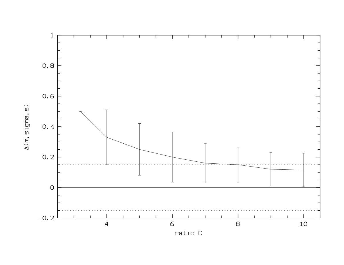
In order to test this point, we have selected the cluster A3158 in an area of 2 Mpc. According to the background level computed in Adami et al. (1998), the ratio (C hereafter) between the background galaxies and the cluster members is 3.7. In this area, the $\Delta_{m,\sigma,s}$ distance is significantly different from 0. We are able to see the structure (Fig. 7).

We increase artificially C by uniformly adding galaxies in the selected field of view. For each set of added galaxies, we make 100 realizations in order to compute an error for $\Delta_{m,\sigma,s}.$ We show in figure 7 the variation of $\Delta_{m,\sigma,s}$ with C. We can see that $\Delta_{m,\sigma,s}$ is significantly different from 0 (according to the error bars) for C$\leq$5. For 5$\leq$C$\leq$7, $\Delta_{m,\sigma,s}$ is different of 0 in more than 50% of the realizations. For C$\geq$7, we are not able to distinguish the cluster structure in more than 50% of the 100 realizations.

We conclude that we are able to make the difference between the cluster and the field even if the ratio C is equal to 5, and probably 7. The influence of a uniform background level is therefore minor.

Figure 7: Variation of $\Delta_{m,\sigma,s}$ for A3158 with different ratio C between the number of background and cluster galaxies.

3.2.2 Clustered contamination

The other possible contamination is those of secondary groups or clusters on the same line of sight. To test this effect, we have build a composite cluster: we have superposed the cluster A0401 (z=0.073) and the cluster A1367 (z=0.023). The contribution of A1367 will then add a signal of structure on the line of sight. We see that we destroy almost all the decrease of $\Delta_{m,\sigma,s}$: the slope of the regression is -0.05$\pm$0.03 (see Table 1). This kind of contamination can erase the variation of the distance $\Delta_{m,\sigma,s}$ with magnitude.

4 Conclusion

We have constructed a fast method, based on the MST, to characterize the aggregation level of sets of galaxies. By using the first 3 momenta of the MST edge length histogram of a given set of galaxies, we are able to discriminate efficiently between different galaxy distributions compare to Poisson ones. The method is not very sensitive to a uniform background contamination. Even with ratio equal of 5 between field galaxies and cluster members, we discriminate the structure. The implications of this first results could be important, in particular to detect possible distant clusters (or structures) in deep photometric survey. The method also shows that the bright galaxies clusters are more aggregated than the faint ones in 75 $\%$ of our selected sample. This result is very coherent with Adami et al. (1998) who show that the bright galaxies in clusters are more aggregated than the faint ones.