Exactly Azimuthal Pixelizations of the Sky

Abstract

We investigate various pixelizations of the sky which allow for fast spherical transforms, for implementation in full sky CMB experiments such as Planck and MAP. We study the effect of varying pixel shape and area on the extraction of the CMB power spectrum. We argue for the benefits of having a truly azimuthal, or ‘igloo’ pixelization. Such pixelizations are simple and allow for fast, exact simulations of pixelized skies. They also allow for precise correction to be made which accounts for the effects of pixel smoothing on extracted multipole moments.

I Introduction

The prospect of high precision all sky maps of the cosmic microwave sky from the MAP and Planck satellites has galvanized cosmology. These maps will contain millions of accurate, independent temperature measurements which can be used to test theories of the early universe and cosmic structure formation. This paper deals with the very practical issue of how to store the data so that it can be easily manipulated and analyzed. In particular we discuss the question of how to pixelize the sky. This is clearly a question of some importance: data of this quantity and quality are likely to form the basis for much of cosmology over the next decade. As we shall discuss, the right choice of pixelization will both dramatically improve and accelerate analysis.

Numerous suggestions for pixelization of the sky have already been made [1, 2]. The simplest uses equal divisions in latitude and longitude ($\theta$ and $\phi$). This has been called the Equidistant Cylindrical Projection (ECP). It has the advantages of being both azimuthal and simply hierarchical, in that the data can be easily coarse grained by combining neighbouring pixels. The azimuthal symmetry allows for fast spherical harmonic transforms, speeding many operations such as map simulation and inversion[3, 4, 5].

The biggest failure of the ECP pixelization is that the pixels near the poles are small and very distorted. In a real experiment, they might be very noisy or even contain no data at all. These extra pixels are also wasteful in later analysis. The ECP scheme can be improved upon by grouping more and more pixels together as one approaches the pole, and this is the idea behind the pixelizations we advocate below.

Previous all sky CMB maps, produced by the COBE satellite, used a pixelization based on the Quadrilateralized Sky Cube Projection, or ‘quad cube’ [2]. The edges of a cube are projected onto a sphere, dividing the sky into six equal areas. These are subdivided into a roughly square, hierarchical lattice. The main drawback of the resulting pixelizations is their lack of azimuthal symmetry, making spherical harmonic transforms time consuming. Other suggested pixelizations have hexagonal instead of square pixels. One is an icosahedral version of the quad cube [6], another is a class based on fullerenes [7]. While these pixels are closest to the ideal, round pixels, they lack azimuthal symmetry or any obvious hierarchical structure for coarse graining.

Gorski and collaborators have recently made available a package of programs, called HEALPIX, which include a novel pixelization scheme based on a rhombic dodecahedron and associated software for performing fast spherical transforms [8]. The centers of the HEALPIX pixels are located on a lattice possessing discrete azimuthal symmetry at each latitude. Such symmetry is essential for making use of Fast Fourier transforms with respect to the azimuthal coordinate $\phi$. However in HEALPIX the pixel shapes vary around circles of constant latitude, so the integrations needed for spherical transforms are only performed approximately, effectively assuming the pixels are azimuthally symmetric, identical and round. In contrast, the pixelizations we consider do possess exact azimuthal symmetry at each latitude, so that we can perform the the integrations needed for spherical transforms exactly.

An attractive feature of the ‘igloo’ schemes we focus on is that they have an exact discrete azimuthal symmetry at each latitude, allowing fast and exact spherical harmonic transforms. In particular, this allows one to rapidly create simulated skies in which the effects of pixels smoothing have been exactly included (up to machine accuracy). The ability to perform such transforms quickly is also likely to be essential to computing the angular power spectrum of the observed sky (for a recent discussion see [9]).

For comparative purposes we consider several different igloo schemes, which satisfy the following criteria to varying extents:

• Lack of Pixel Distortion – Pixelization of the data suppresses modes with wavelengths shorter than the pixel dimensions in any given direction. To minimize this effect one should try to make the largest pixel diameter as small as possible. The ideal (unachievable) limit would be to have circular pixels where the largest diameter is $D=4/\sqrt{N_{tot}}$ where $N_{tot}$ is the total number of pixels on the sky. (One can see this by considering the average pixel area, $A=4\pi/N_{tot}=\pi D^{2}/4$.) For square pixels, the best one can achieve is $D=\sqrt{8\pi/N_{tot}}$, about 25% larger. In general we define the distortion of a pixel to be the length of longest diameter divided by this ideal value $D$.

• Equal Area Pixels – This is desirable in order to get the best resolution for a fixed number of pixels, and so that the pixels, in the first approximation, have equal statistical weight. However, since sky coverage and and foregrounds are unlikely to be uniform, it is not clear that exactly equal area pixels are essential.

• Built-in Hierarchy – A hierarchical pixelization scheme allows for coarse graining of the data at different resolutions. This is likely to be at least very useful, and probably essential, in analyzing the data. We require that the hierarchy be nested, that is that each higher resolution pixels should fit perfectly into a single lower resolution pixel. Ideally one would like the hierarchy to coarsen to as small a base set of pixels as possible, maintaining minimal distortion and roughly equal area pixels at each level.

In section II, we describe the general features of igloo pixelizations as well as specific characteristics of the models that we consider here. In section III, we present some general considerations for creating and inverting pixelized maps, and describe how the azimuthal symmetry can be exploited. Finally, in section IV, we create and invert realistic maps with the various pixelizations and examine the accuracy with which the power spectra can be extracted.

II Igloo Tilings

A General Description

By an igloo pixelization, we mean one divided into rows with edges of constant latitude and where each row is divided into identical pixels by lines of constant longitude. The pixels are roughly trapezoidal shaped, becoming nearly rectangular away from the poles. For simplicity and to speed calculations, the northern and southern hemispheres are tiled identically.

Igloo tilings have many advantages. First, they are quite simple. They are also naturally azimuthal and can be easily made equal area, with most pixels nearly square. But perhaps their biggest advantage is that the pixel edges are defined along constant lines of the spherical polar coordinates $\theta$ and $\phi$, allowing for an exact, fast integration of spherical harmonics over the pixels. This is essential in constructing exact simulated skies, and in optimally recovering the sky power spectrum from real data.

The simplest example of an igloo pixelization is the ECP pixelization itself, which we will include in our comparison. In it, every row has the same number of pixels, and the pixels become quite narrow near the poles. The other models we consider have pixels which are more nearly square and nearly (or exactly) equal area. To do this the number of pixels in each row must decrease as one approaches the poles (Figure 2).

One can construct igloo pixelizations with either rows equally spaced in latitude, like the ECP, or with pixels of uniform area. The advantage of equal latitude spacing is that the pixelization can be created by a simple rebinning of an ECP pixelization, providing the latter is chosen to have an appropriate number of pixels. In addition, by letting the pixel areas vary, one can make them less distorted. An equal area pixelization will not be exactly equally spaced in latitude, but has the advantage that all of the pixels will have the same statistical weight.

Igloo pixelizations can also be made hierarchical. To do this, one first divides the sphere into a base pixelization with relatively few pixels, optimized to minimize the pixel distortion. Each of these coarse pixels is then divided into four by bisecting it in longitude and latitude. The latter division is chosen either to keep the pixels the same area or to maintain a constant latitude spacing of the rows. Thus one creates a finer grained pixelization with four times the number of pixels. This procedure can be repeated until we reach the required resolution.

Reducing the number of base pixels tends to increase the level of pixel distortions, so some compromise must be found. While there are clear advantages to having fewer base pixels, it is not obvious how they should be weighed against the advantages of having more uniform pixels. Here, we will consider two possible extremes, pixelizations with twelve base pixels (roughly $60^{o}\times 60^{o}$ each), and one with 12,116 $2^{o}\times 2^{o}$ base pixels. The latter number was chosen because an analysis at this resolution is comparable to what has already been accomplished for COBE, and it is unlikely one will need an analysis at a lower resolution.

The hierarchical division causes some of the subpixels to become more distorted than the coarser pixels, especially near the poles. Away from the poles, there is a limit to how distorted the pixels become, even at the highest resolutions. However, if the polar cap were simply bisected in $\theta$ and $\phi$, the pixels would become more and more distorted, as occurs in the ECP. Thus, we must use another method for dividing the polar regions.

In our pixelization, we have chosen to initially divide the cap of each pole into three equal wedges. Higher resolution pixelizations are found by dividing each wedge into four pieces, one central wedge and three pieces surrounding it. (See Figure 1.) This process is iterated, with the interior wedge always being divided in this way and the outer pieces being divided by lines of constant $\theta$ and $\phi$. This prescription is designed in order to minimize the distortions in the highest resolution pixels.

FIG. 1.: Picture of the polar cap region in the igloo schemes, showing three levels of subdivision to higher resolution pixels.

B The Base Pixelization

We would like to begin with base pixels that are as uniform and undistorted as possible. We can make the pixels nearly square by choosing the right number of pixels in each row. The best number at a given latitude is given by the distance around the sphere at that latitude divided by the width of each pixel. Thus, if the average area of each pixel is $A=4\pi/N_{tot}$, then the ideal number in a row at angle $\theta$ is $N(\theta)=2\pi\sin(\theta)/\sqrt{A}=\pi^{1/2}\sin(\theta)\sqrt{N_{tot}}$. Since the number of pixels must be an integer, some slight distortion of the pixels is inevitable.

If we treat the region near the pole as effectively flat, then it is simple to calculate the ideal numbers in the concentric layers. Assuming the pixels are square, the radius for each layer increases by $\sqrt{A}$, so that the ring area increases by $2\pi A$. Thus, the number in a layer is related to the number in the previous layer by $N_{p}=N_{p-1}+2\pi$. If the cap is initially divided into three wedges, the next row should contain nine pixels, and there should be roughly six more pixels in each additional row. The precise numbers are chosen to minimize pixel distortion at the highest resolutions. One possible sequence might be 3, 9, 15, 22, 28, 34, 40, 46…

Having arbitrary integers in the rows reduces the effectiveness of Fast Fourier Transforms (FFTs), whose speed depends on the number of pixels in a row being a product of low primes. To minimize this effect, one should be selective in choosing the number of pixels allowed in a row. For example, we may chose only numbers of the form, $2^{n}$ or $3^{m}\times 2^{n}$. Since allowing more possibilities reduces the amount of pixel distortion, one might alternatively consider all numbers which do not have large prime factors. For example, in the 12,116 base pixel model we exclude only numbers with prime factors bigger than 23.

We parameterize the distortion in terms of the largest pixel diameter, $D$, which is related to the pixel height, $h$, and its width, $w$: $D^{2}\simeq h^{2}+w^{2}$. The width is given by $w=2\pi\sin(\theta)/N_{p}=\sqrt{A}N(\theta)/N_{p}$, where $N(\theta)$ is the ideal number of pixels at a given latitude and $N_{p}$ is the actual number. In the equal latitude pixelizations, the pixel height is fixed (ideally at $h=\sqrt{A}$,) so that

$$D^{2}\simeq A(1+(N(\theta)/N_{p})^{2}).$$ (1)

In the equal area case, the height varies inversely with the width, so that

$$D^{2}\simeq A((N_{p}/N(\theta))^{2}+(N(\theta)/N_{p})^{2}).$$ (2)

The distortions are smaller on average in the constant latitude case, but the pixel areas vary from row to row.

If one allows large number of base pixels, then the pixel widths and heights can be made almost equal ($D^{2}={2A}$) for most of the pixels, with the distortions being the worst at the poles. Even in the finest subdivision however, the pixel distortions do not become arbitrarily bad. The most distorted pixels never have diameters larger than about $D^{2}\simeq 4A$ in any of the pixelizations we consider, and these are relatively rare.

These pixelizations are optimized to be both azimuthal and hierarchical. The data need to be ordered differently depending on which of these properties we are interested in utilizing. For the creation and analysis of maps, it is helpful to have an azimuthal ordering. However, to facilitate coarsening, one would reorder the data into chunks associated with the coarsest graining. Within these chunks, the data would be ordered like each face in the quad cubed, so that adding the data in groups of four converts it to the next coarser level.

C Specific Igloo Tilings

For definiteness, here we consider four possible igloo pixelizations:

• an ECP pixelization

• a twelve pixel scheme (3:6:3) divided with equal area

• a twelve pixel scheme (3:6:3) divided with equal latitude spacing

• an equal area scheme with 12,116 base pixels

In the twelve pixel scheme, the base pixels are arranged as shown in Figure 2 (bold lines), with three pixels at each cap and six around the center. The divisions between the layers lie at $\theta=\pm 30^{\circ}$. (We note that the pixelizations recently suggested by Gorski [8] also involve twelve base pixels, but arranged instead in rows of 4:4:4.) To facilitate comparisons, the ECP model was chosen to have nearly the same number of pixels as the other models, and was based on a $5\times 10$ grid, with the base pixels having edges of $\Delta\theta=\Delta\phi=36^{\circ}$.

FIG. 2.: Picture of the 3:6:3 equal area pixelization, which divides the sky into twelve base patches, three at either cap and six $60^{o}\times 60^{o}$ patches at the equator. Here, each base pixel is broken up into 64 smaller pixels.

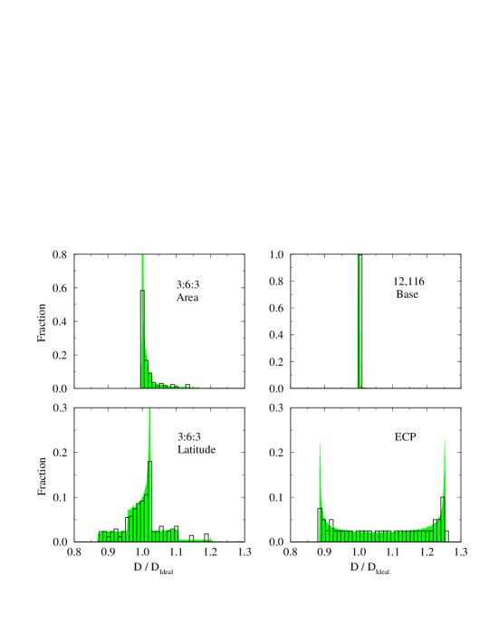
Distortions: We evaluate these schemes given roughly equal numbers of pixels in each. We expect naively that the quality of the pixelization should depend on the average diameter of the pixels. Figure 3 shows the percentage of pixels with a given maximum diameter for the various models.

The least distortions result from the pixelizations with the greatest number of base pixels, and for 12,116 base pixels the amount of distortions is very close to the ideal (square) result. When the number of base pixels is reduced to twelve, greater distortions result. In the equal area case, the minimum diameter is fixed and grows larger for pixels that are less square. In the equal latitude case, the distortions are comparable. However, the pixels with less area can have a smaller diameter, so that the average diameter is actually smaller than in the equal area case. Finally, the distortions in the ECP are the largest because many of its pixels contain very little area, which makes the remaining ones larger.

FIG. 3.: The percentage of pixels with a given maximum diameter for each of the pixelizations, normalized in terms of the ideal diameter for square pixels, $D_{Ideal}=\sqrt{8\pi/N_{tot}}$. The histograms show the distribution for $2^{\circ}$ pixelizations, while the shaded region shows the results when each component pixel is divided into 1024 subpixels ($3.5^{\prime}$ resolution.)

FIG. 4.: The distribution of the area of the pixels for the unequal area models. The top figure is normalized so that the average area is one, while the bottom figure is normalized so that the area of the pixels along the equator is one. Again, the histograms show the distribution for $2^{\circ}$ pixelizations, while the shaded region shows the results when each component pixel is divided into 1024 subpixels.

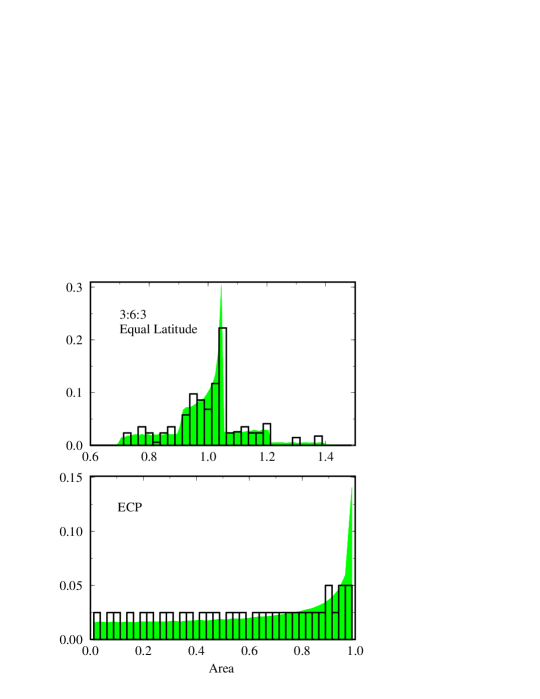
Area: Only two of these pixelizations, the twelve pixel equal latitude and the ECP pixelization, are not equal area by construction. We might hope that variations in pixel area themselves will have little effect, because we calculate the spherical transforms properly weighting for the different pixel areas. Nevertheless the ECP scheme is at a disadvantage because the large number of small pixels implies that, for a fixed number of pixels, the largest pixels (and the average pixel diameter) are bigger than in the other models. Figure 4 shows the distribution of area for the ECP and the equal latitude 3:6:3 scheme. While the pixel areas do vary in the equal latitude 3:6:3 scheme, they do so in a way which keeps the pixel distortion small.

Hierarchy: In regards to hierarchy, the best pixelization is the ECP, which in its simplest implementation can be reduced to just two pixels, the East and West hemispheres. The 3:6:3 models are nearly as good, having only twelve base pixels. Of the two, the equal latitude case is somewhat simpler and has the advantage that it can be subdivided into an ECP pixelization with $(3\times 6)2^{n}$ pixels. Clearly, the poorest pixelization in this regard is the 12,116 base pixelization, which only coarsens down to two degree patches, and so requires more information to specify uniquely.

III Evaluating Pixelizations

The criteria we use to judge the various pixelizations are the speed and accuracy with which one can create and invert realistic sky maps. Any reasonable pixelization should do well in finding the low multipoles which do not vary appreciably over the pixels. The true test is how well one can extract the power spectrum at high multipoles, corresponding to wavelengths on the sky approaching the dimensions of the pixel.

To evaluate different pixelizations, we create realizations assuming Gaussian statistics and a sample (CDM) power spectrum. The simulated multipole coefficients are then exactly transformed into pixelized maps. We then perform an exact spherical transform of the pixelized maps to attempt to recover the initial power spectrum. In this final step, errors occur in two ways. First, the pixelized maps contain only $N_{tot}$ numbers: information regarding modes whose wavelength is shorter than the pixel size has been lost. Second, when one attempts to correct the recovered multipole coefficients for the effect of pixel smoothing, one can do so at various levels of approximation (and speed), as will be discussed below.

A General Considerations

Two maps must be considered, the true map of the temperature on the sky, and the map projected into the pixelization of the sky. The true continuous temperature can be expressed as

$$T(\theta,\phi)=\sum_{l,m}a_{lm}Y_{lm}(\theta,\phi)$$ (3)

where the $a_{lm}$’s are variables that are Gaussianly distributed with zero mean and variance given by the power spectrum, $\langle|a_{lm}|^{2}\rangle=C_{l}.$ This can be inverted using the orthogonality of the spherical harmonics to find

$$a_{lm}=\int T(\theta,\phi)Y^{*}_{lm}(\theta,\phi)d\Omega.$$ (4)

For our present purposes, the true map is the sky smoothed by the experimental window function. The two point correlation function is

$$\langle T(\Omega)T(\Omega^{\prime})\rangle = \sum_{lm}C_{l}Y_{lm}(\Omega)Y^{*}_{lm}(\Omega^{\prime})$$ (5)

$$= {1\over 4\pi}\sum_{l}(2l+1)C_{l}P_{l}(\cos\theta_{\Omega\Omega^{\prime}}),$$ (6)

where $\theta_{\Omega\Omega^{\prime}}$ is the angular separation of the two points.

Unfortunately, the true map is not directly observable. Experiments will produce pixelized maps where the temperature in each pixel is the true temperature averaged over the area of the pixel. The measured temperature in one of these pixels is given by

$$T_{P}=\int W^{P}(\theta,\phi)T(\theta,\phi)d\Omega$$ (7)

where $W^{P}(\theta,\phi)$ is the pixel window function for the P^th pixel, equal to $1/A_{P}$ (where $A_{P}$ is the area of the pixel) within the pixel and zero otherwise. Thus, $T_{P}$ is the average of the temperature in the pixel. Expanding the temperature in terms of spherical harmonics, we find

$$T_{P} = \int W^{P}(\theta,\phi)\sum_{l,m}a_{lm}Y_{lm}(\theta,\phi)d\Omega$$ (8)

$$= \sum_{l,m}a_{lm}W^{P}_{lm}$$ (9)

where $W^{P}_{lm}$ is defined by $W^{P}_{lm}=\int d\Omega W^{P}(\theta,\phi)Y_{lm}(\theta,\phi)$ and $W^{P}(\theta,\phi)=\sum W^{P}_{lm}Y^{*}_{lm}(\theta,\phi).$ The vector $W^{P}_{lm}$, $P=1,..N_{tot}$, is the pixelized analog of the continuous function $Y_{lm}(\theta,\phi)$.

The pixelized analog to the two point correlation function is the pixel-pixel correlation,

$$\langle T_{P}T_{Q}\rangle=\sum_{lm}C_{l}W^{P}_{lm}W^{Q*}_{lm}.$$ (10)

In general, this cannot be further simplified because the pixelization breaks rotational invariance. For the special case of white noise, $C_{l}=C_{WN}$ is constant, and the pixel-pixel correlation is simply $C_{WN}\delta_{PQ}/A_{P}$.

While the pixelized map is discrete, it is a well defined function on the sky and can itself be expanded in terms of orthogonal functions:

$$T^{pix}(\theta,\phi) = \sum_{P}T_{P}A_{P}W^{P}(\theta,\phi)$$ (11)

$$= \sum_{l,m}a^{pix}_{lm}Y_{lm}(\theta,\phi).$$ (12)

This can be inverted to find that

$$a^{pix}_{lm} = \int T^{pix}(\theta,\phi)Y^{*}_{lm}(\theta,\phi)d\Omega$$ (13)

$$= \int\sum_{P}T_{P}A_{P}W^{P}(\theta,\phi)Y^{*}_{lm}(\theta,\phi)d\Omega$$ (14)

$$= \sum_{P}T_{P}A_{P}W^{P*}_{lm}.$$ (15)

This is the pixelized analog of equation (3.2). In principle, all the pixelized multipoles, an infinite number of them, are well defined and could be calculated. However, since there are only $N_{tot}$ independent pixel temperatures, only a finite number of the extracted $a_{lm}^{pix}$’s can be linearly independent, which we can take to be the lowest $N_{tot}$ $a^{pix}_{lm}$’s (i.e. with $l$ up to $l=\sqrt{N_{tot}}-1$).

The pixelized multipoles can be related to the true multipoles by substituting the above expression for $T_{P}$,

$$a^{pix}_{lm}=\sum_{l^{\prime}m^{\prime}}a_{l^{\prime}m^{\prime}}\sum_{P}A_{P}W^{P*}_{lm}W_{l^{\prime}m^{\prime}}^{P}.$$ (16)

This equation tells us that the $a^{pix}_{lm}$ are special linear combinations of the true underlying $a_{lm}$’s we are interested in. A pixelized map can only provide a finite number of constraints on the infinite number of possible multipoles which might exist. We cannot recover the underlying $a_{lm}$’s without making an additional assumption, the simplest being that they are all zero beyond some value of $l$. This is perhaps the most natural choice, because while all the multipoles might in principle be non-zero, the highest multipoles will eventually be suppressed due to the finite resolution of the antenna and the pixel size. (If higher multipoles are present, then these will mimic combinations of the lower multipoles and so will reduce the accuracy to which they can be extracted.) With this assumption, we can attempt to solve equation (16) for the true $a_{lm}$’s.

One possible way to solve equation (16) for the $a_{lm}$’s exactly is by iteration, making a guess for the $a_{lm}$’s and then making a correction based on that guess. Consider the positive semi-definite function

$$f=\sum_{P}A_{P}T_{P}^{2}({\rm error})$$ (17)

where $T_{P}({\rm error})$ is the temperature difference between the measured temperature on the $P$’th pixel and the temperature one would get given some guess for the $a_{lm}$’s,

$$T_{P}({\rm error})=T_{P}({\rm guess})-T_{P}({\rm true}).$$ (18)

The scheme to solve (16) is then just to minimize the function $f$ in (17), which can be straightforwardly calculated for any conjectured set of $a_{lm}$’s using the fast Fourier transforms described below. The minimization of $f$ can be done iteratively in a very simple manner, and we report on results from this method below.

One danger in making this inversion is that the multipoles we have chosen to extract might not fully span all the degrees of freedom of temperature map. If this were the case, the matrix in equation (16) is singular and cannot be inverted. For example, two apparently orthogonal functions might appear identical when they are pixelized, making a unique inversion for the $a_{lm}$’s impossible. In reality, this degeneracy of functions will only be approximate, but it will make solving for the underlying $a_{lm}$’s difficult. To minimize these dangers, it makes sense for the ideal pixelization to represent all the multipoles we have chosen to solve for (those below $l\leq\sqrt{N_{tot}}-1$) as orthogonally as possible.

While it is important that in principle a scheme exists for solving (16) exactly for the $a_{lm}$’s (modulo the necessary assumption that they vanish for high $l$), in practice one may be more interested in a fast scheme for recovering the $a_{lm}$’s approximately. When the spherical harmonics do not vary much across the pixels (i.e., for low $l$), then the orthogonality of the spherical harmonics, $\int d\Omega Y_{lm}Y^{*}_{l^{\prime}m^{\prime}}=\delta_{mm^{\prime}}\delta_{ll^{\prime}}$ implies that

$$\sum_{P}A_{P}W^{P*}_{lm}W_{l^{\prime}m^{\prime}}^{P}\simeq N_{lm}\delta_{ll^{\prime}}\delta_{mm^{\prime}},$$ (19)

where, $N_{lm}\equiv\sum_{P}|W^{P}_{lm}|^{2}A_{P}$. In this case, the inversion can be found to be

$$a^{est}_{lm}\simeq{\sum_{P}T_{P}A^{P}W^{P*}_{lm}\over N_{lm}}.$$ (20)

This relation naturally breaks down at high multipoles, when the number of multipoles to be extracted approaches the number of pixels.

One can estimate the power spectrum from these extracted multipole moments. The naive estimate is simply,

$$C_{l}^{est}\equiv{1\over(2l+1)}\sum_{m}|a^{est}_{lm}|^{2}.$$ (21)

Unfortunately, this estimator is biased and tends to overestimate the power spectrum, especially at high multipoles. This is easy to understand. Suppose one has a single mode on the sky, which is then pixelized. The lack of orthogonality of the modes projected on the pixelization implies that when inverting the pixelization, one would recover the original mode, plus an admixture of small contributions to other modes. The latter tend to increase the extracted power. One can construct an unbiased estimator from $C_{l}^{est}$ (or from $C_{l}^{pix}$.) It can be shown that

$$\langle C_{l}^{est}\rangle={\cal M}_{ll^{\prime}}C_{l^{\prime}}$$ (22)

where,

$${\cal M}_{ll^{\prime}}\equiv{1\over(2l+1)}\sum_{mm^{\prime}}{1\over N_{lm}^{2}}\sum_{P}A_{P}W^{P*}_{lm}W_{l^{\prime}m^{\prime}}^{P}\sum_{Q}A_{Q}W^{Q}_{lm}W_{l^{\prime}m^{\prime}}^{Q*}.$$ (23)

This matrix is a function of the pixelization alone, so need be calculated only once. Given this matrix, an unbiased estimator of the power spectrum is

$$C_{l}^{unbiased}={\cal M}^{-1}_{ll^{\prime}}C^{est}_{l^{\prime}}.$$ (24)

This removes the systematic effect of leakage from other multipoles and is quick to calculate. However, it ignores off-diagonal correlations between the $a_{lm}^{est}$’s, and so is not the best possible estimator of the power spectrum.

B Azimuthal Pixelizations

For azimuthal pixelizations, it is helpful to replace the general pixel index $P$, with two indices $p,q$ where the former represents the row number and the latter identifies the pixel within that row. Each row has $N_{p}$ identical pixels placed periodically in $\phi$. We can expand the spherical harmonics as

$$Y_{lm}(\theta,\phi)=\lambda_{l}^{m}(\cos\theta)e^{im\phi},$$ (25)

where $\lambda_{l}^{m}(x)$ are the normalized Legendre polynomials, defined in terms of the associated Legendre polynomials by

$$\lambda_{l}^{m}(x)=\left({(2l+1)\over 4\pi}{(l-m)!\over(l+m)!}\right)^{1/2}P_{l}^{m}(x),$$ (26)

following the notation of Muciaccia, Natoli and Vittorio (MNV, 1997).

The window functions in azimuthal pixelizations can be easily calculated.

$$W^{pq}_{lm} = \int d\Omega W^{pq}(\theta,\phi)Y_{lm}(\theta,\phi)$$ (27)

$$= {1\over A_{p}}\int^{2\pi q/N_{p}}_{2\pi(p-1)/N_{q}}e^{im\phi}d\phi\int^{\theta_{p+1}}_{\theta_{p}}\lambda^{m}_{l}(\cos\theta)\sin\theta d\theta$$ (28)

$$= e^{imq2\pi/N_{p}}W^{p}_{lm}$$ (29)

where we have defined the $q$ independent part of the window function as,

$$W^{p}_{lm}=e^{im\pi/N_{p}}{\sin(\pi m/N_{p})\over(\pi m/N_{p})}{1\over\Delta x_{p}}\int^{\theta_{p+1}}_{\theta_{p}}\lambda^{m}_{l}(\cos\theta)\sin\theta d\theta,$$ (30)

and $\Delta x_{p}=\cos(\theta_{p+1})-\cos(\theta_{p})$. The final integral can be evaluated very quickly in a recursive fashion, comparable to the time required to evaluate the Legendre functions themselves. (See appendix A.) The ability to exactly integrate over the pixels quickly is an important advantage of the igloo class of tilings.

It is the simple dependence on $q$ of the window functions that allow the creation and inversion of maps to be evaluated using Fast Fourier Transforms. To take advantage of this in creating maps, it is useful to rewrite the expression for the pixel temperature, reordering the sums in a suggestive way (again adapting the notation of MNV):

$$T_{pq} = \sum_{l=0}^{l_{max}}\sum_{m=-l}^{l}a_{lm}W^{p}_{lm}e^{imq2\pi/N_{p}}$$ (31)

$$= \sum_{m=-l_{max}}^{l_{max}}\sum_{l=|m|}^{l_{max}}a_{lm}W^{p}_{lm}e^{imq2\pi/N_{p}}$$ (32)

$$= \sum_{m=-l_{max}}^{l_{max}}b_{m}(\theta_{p})e^{imq2\pi/N_{p}}.$$ (33)

Here,

$$b_{m}(\theta_{p})=\sum_{l=|m|}^{l_{max}}a_{lm}W^{p}_{lm}=\sum_{q}T_{pq}e^{-imq2\pi/N_{p}},$$ (34)

and the transformation between $b_{m}(\theta_{p})$ and $T_{pq}$ can be made with a FFT. However, since there are only a limited number of pixels, only the frequencies $-N_{p}/2\leq m\leq N_{p}/2$ can be represented on the lattice. When the number of modes exceeds $N_{p}/2$, the modes appear on the lattice like modes with frequency $mod(m,N_{p})$ and their power must be aliased into these lower frequencies.

Since the northern and southern hemispheres are tiled in the same way, we can use this symmetry to save a factor of two in computing time [4]. The associated Legendre polynomials are even or odd functions across the equator, depending on whether $l+m$ is an even or odd number. We can break the $b_{m}(\theta_{p})$ functions into even and odd pieces and evaluate them in only the northern hemisphere, and find the full function by

$$b_{m}(\theta_{p},{\rm north}) = b_{m}(\theta_{p},{\rm even})+b_{m}(\theta_{p},{\rm odd})$$ (35)

$$b_{m}(\theta_{p},{\rm south}) = b_{m}(\theta_{p},{\rm even})-b_{m}(\theta_{p},{\rm odd}).$$ (36)

The inversion of the maps can be performed similarly,

$$a_{lm} = {1\over N_{lm}}\sum_{pq}T_{pq}A^{p}W^{pq*}_{lm}$$ (37)

$$= {1\over N_{lm}}\sum_{p=1}^{n_{rows}}A^{p}W^{p*}_{lm}\sum_{q}T_{pq}e^{-imq2\pi/N_{p}}$$ (38)

$$= {1\over N_{lm}}\sum_{p=1}^{n_{rows}}b_{m}(\theta_{p})A^{p}W^{p*}_{lm}.$$ (39)

Similarly, care must be taken in the inversion to map the power from the lower modes to the higher ones.

It is the effect of the higher modes on the pixelization mimicking the lower ones which is primarily responsible for making the exact inversion of the map impossible. In the continuous case, the orthogonality of the spherical harmonic functions is enforced in two ways: first, the azimuthal functions ($e^{im\phi}$) are orthogonal for $m\neq m^{\prime}$ and second, when $m=m^{\prime}$ (and only then), the Associated Legendre functions are orthogonal for $l\neq l^{\prime}$. In the pixelized case, this remains approximately true when $m,m^{\prime}\leq N_{p}/2$, but this breaks down for larger modes, so that modes with $m\neq m^{\prime}$ are not necessarily orthogonal. Then the lack of orthogonality for the Legendre polynomials means these functions can appear to be the same.

To minimize this effect, it is helpful to have as many pixels per azimuthal row as possible. For the equal area models we consider, each pixel has an area of $4\pi/N_{tot}$, with edges of length $\sqrt{4\pi/N_{tot}}$. Thus there are $\sqrt{\pi N_{tot}}$ pixels along the equator, and the problem of orthogonality becomes a serious problem near the Nyquist frequency at the equator, $l\simeq N_{equator}/2=\sqrt{\pi N_{tot}}/2$. This is close to the maximum we could reasonably hope for given the finite number of pixels, $l\simeq\sqrt{N_{tot}}$.

The normalization of each mode can be found quickly from the expression,

$$N_{lm}=\sum_{p=1}^{n_{rows}}A_{p}W^{p*}_{lm}W_{lm}^{p}N_{p}.$$ (40)

For round pixels, the normalization is independent of $m$ and this is usually assumed for the sake of simplicity. In a more realistic pixelization, however, there can be large variations for different $m$’s, especially at high multipoles. Thus, the ability to calculate these individual normalizations is a great advantage in making an inversion.

IV Results

We begin by showing the average normalization, $\sum_{m}N_{lm}/(2l+1)$, for the various pixelizations. This illustrates the average suppression of modes by the pixelization and is equivalent to its window function. The mean window functions are virtually identical for all the pixelizations with the exception of the ECP which falls off slightly more quickly. The shape of these curves reflects primarily the effective area of the pixels, and while the ECP has the same average area, its skewed distribution of shapes makes them dominated by the larger pixels.

FIG. 5.: Figure of $N_{lm}$ averaged over $m$ as a function of $l$ for each pixelization. The error bars indicate the variance of $N_{lm}$ for the different values of $m$. (Based on roughly 49,000 pixels.)

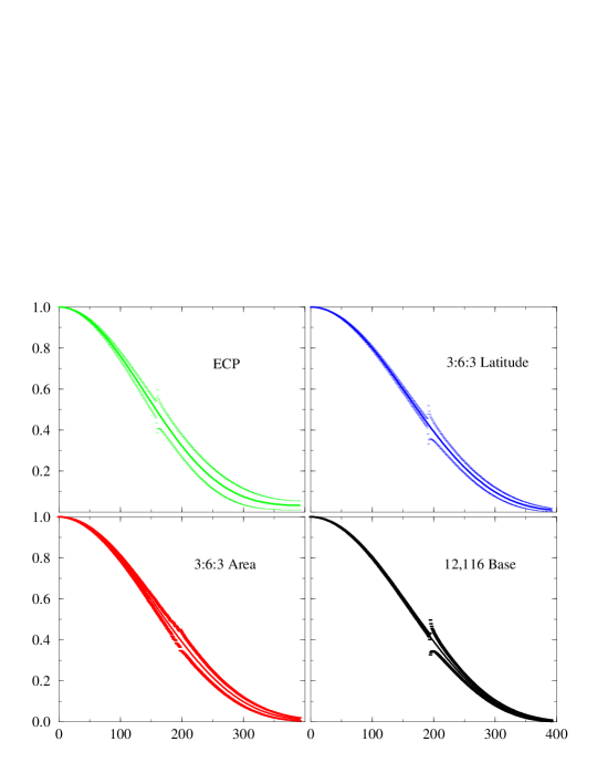
A more pronounced difference appears in the variance of the window functions for a fixed $l$, as indicated by the error bars. This is correlated with the average amount of distortion of the pixelization, with the ECP having the largest variance and the 12,116 base the least. In addition, a feature appears in the variance of the window functions precisely at $l_{Nyquist}$, when particular modes can be either in phase or out of phase with the pixelization.

To minimize aliasing of the higher multipoles, the ideal window function would be zero above a given cutoff in $l$ ($=\sqrt{N_{tot}}$,) so that the pixelization would have no response to the higher modes. However, we have been assuming the pixels have a sharp cutoff in real space, which makes aliasing from higher $l$ modes inevitable. For both the temperature map and its Fourier transform to be as local as possible, it could be advantageous for the window function to be effectively Gaussian, falling off both at large distances and at high multipoles. However, such a scheme would make eliminating foregrounds more difficult.

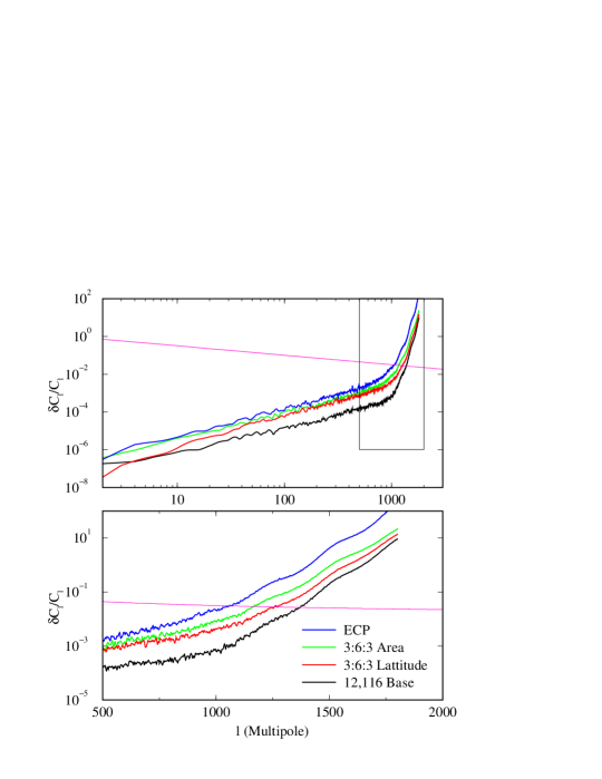
How well can we recover an input power spectrum? We first consider inverting using the fast, approximate approach described in equation (20). Figure 6 shows the errors in inverting the power spectra using that technique for the four models we are considering. Here and below, we plot the fractional error in the estimated multipole, $(C_{l}^{est}-C_{l}^{made})/C_{l}^{made}$ and take the absolute value when plotting on a log scale. For this figure we have assumed a standard CDM power spectrum with a smoothing of $6^{\prime}$. We compare the various pixelizations with approximately three million pixels in each. The accuracy seems to follow a power law ($\propto l^{2}$) at small multipoles and then rises quickly at higher multipoles, when the orthogonality of the modes breaks down and the power spectrum is systematically overestimated. At these multipoles, aliasing due to the other multipoles cannot be ignored.

As one might expect, due to the larger average diameter, the ECP pixelization performs worst of the models we consider, for fixed number of pixels. The best performing model is the 12,116 base pixel model, which has been shown to have the least pixel distortions and has exactly equal area. It is able to invert the power spectrum an order of magnitude better than the other models considered for most of the multipoles. In the middle range lie the 3:6:3 models, which have a smaller diameter than the ECP model, but are more distorted than the large base pixel model. Here, the equal latitude model works somewhat better than the equal area models, implying that the diameter of the pixels is a key factor evaluating the pixelizations.

For comparison, we also include a rough measure of the level of cosmic variance which occurs because we can only measure a finite number of multipoles for a given $l$. This sample variance drops roughly as $\delta C_{l}\sim C_{l}/\sqrt{l}$. At low $l$, the uncertainties in extracting the multipoles are far outweighed by the sample variance. These converge as one goes to higher and higher $l$. While the errors from the pixelization can be generally be made much smaller than the cosmic variance, they can not be ignored if they are systematic in nature.

FIG. 6.: Figure of the errors in extraction of the $C_{l}$ for the various pixelizations with roughly three million pixels in each. The boxed section is enlarged in the lower plot. The cosmic variance ($\delta C_{l}\sim C_{l}/\sqrt{l}$) error level is shown the descending line, while the highest rising line shows the effect of not using the exact window functions. The results are the average of five runs each, and are smoothed for clarity.

FIG. 7.: The scaling of the accuracy of the inversion for different resolutions for two pixelizations. Note that the features that seem to occur at particular multipoles are due to the particular seeds used to create the maps rather than features inherent in the pixelization. Shown are results for pixelizations with roughly $12,000\times(1,4,16,64,256)$ pixels.

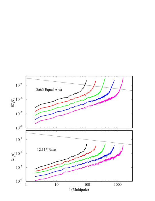
It important to understand how these conclusions change when the resolution increases, keeping the same base number of pixels. Figure 7 shows two of the pixelizations for a range of resolutions, from $2^{\circ}$ to 7’. To good approximation, the effect of increasing the number of pixels by four is to shift the curves to higher $l$ by a factor of two. (The residual differences between the curves is likely to be due to the varying shape of the input power spectrum.) At low $l$, increasing the number of pixels by a factor of four decreases the errors in the extracted power by approximately the same factor.

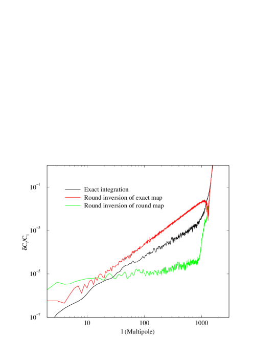
Our results are qualitatively different from those found by MNV, who found the percentage errors were roughly constant as a function of $l$. This is likely because they were creating and inverting the maps using the same assumptions, evaluating the spherical harmonics in the center of the pixels, rather than integrating over the pixels as we do here. In this approach, pixel smoothing can be approximated by assuming the pixels are uniform round tophats with the same area of the the true pixels. However, creating the maps in this way effectively ignores the true pixel shapes and leads to a sizable underestimation of the errors arising from the pixelization. Figure 8 shows the effect of inverting such a realistic map by assuming round pixels. One can see that the effect of this is to greatly reduce the accuracy of the inversion, even for the lowest multipoles. The systematic error introduced by using an inaccurate window function appears to dominate the statistical errors.

When testing the quality of their inversions, previous analyses have assumed that the power spectrum of the initial maps cuts off precisely at the Nyquist frequency on the equator, $l_{Nyquist}=N_{equator}/2$. Thus, they have only put in the power that they could extract. However, this is not a realistic assumption – the higher multipole modes exist and must be included to understand the accuracy of the extracted power spectrum. Though these modes tend to be damped by experimental and pixel smoothing, even when the pixel size is much smaller than the beam size the spectrum falls off smoothly rather than sharply. Thus, the power above any given cutoff is always comparable to that just below it and cannot be ignored. The presence of these higher modes can adversely affect the inversion because they can mimic the lower modes on the pixelization.

FIG. 8.: We show the effects of approximating the pixels as round tophat pixels with the same average area. If one creates and inverts the maps using this assumption, one finds very good accuracy compared to the exact results. These results are deceptive, however, because they ignore the true pixel shapes. If one creates the maps by integrating over the true pixel shapes, and inverts assuming the pixels were round tophats, the accuracy is much worse than the exact results.

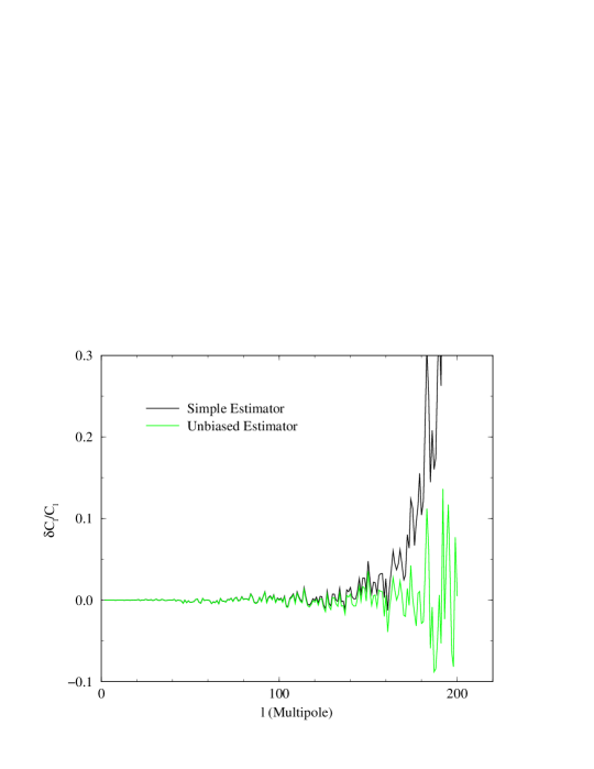
The presence of the higher modes can be corrected for, in part, by using the unbiased estimator defined in equation (24). Figure 9 shows the errors in the recovered power spectra with and without correcting for this bias. Without the correction, the power spectrum is greatly overestimated at high frequencies. With the correction, the power spectrum can be recovered even beyond $l_{Nyquist}$, though with decreasing accuracy.

FIG. 9.: The simple estimator for the power spectrum is biased by the presence of other modes, which leads to systematically overestimating the power. Corrected for this bias greatly reduces the error at high $l$. (Based on $N_{tot}=49,152$ pixels, with $l_{Nyquist}=192$.)

We have been comparing models assuming they have nearly the same numbers of pixels. Rather than using the number of pixels as our criterion, it might be fairer to compare pixelizations for a given speed, or equivalently a given number of azimuthal rows. For example, the ECP pixelization has $\sim$ 20% fewer rows than the other models we considered and would perform much better if it had the same number of rows, when it would have 50% more pixels. This would improve its accuracy, making it comparable to the 12,116 base model. It is worth considering whether for a given pixelization one should increase the number of pixels per row, which would improve the orthogonality of spherical harmonics without adding much to the computation time. (Though, some it would not improve much, for example the $m=0$ modes.) If one chooses to make the pixels more narrow, however, it would be better to do it in a uniform way for all of the pixels, rather than just at the poles, as the ECP pixelization does.

Finally, we have also attempted to invert equation (16) directly rather than only approximately. We constructed simulated skies in which we set the $a_{lm}$’s equal to zero beyond some cutoff value $l_{c}$ and used an iterative scheme described in [10] to find the minimum of the function $f$, defined in equation (17), taking advantage of the sparseness of the matrix. One difficulty in an exact inversion is that as $l_{c}$ approaches $\sqrt{N_{tot}}$, the number of directions in which $f$ is flat grows. That is, some particular linear combinations of $a_{lm}$’s have very little impact on the pixelized temperatures: the pixelization effectively washes out these combinations. These multipoles are thus very difficult to extract.

To overcome this problem, we conduct a number of trial simulations and minimizations, and compute the fractional error $\langle|\delta a_{lm}|^{2}\rangle/C_{l}$ for each $l$ and $m$. Modes where this fractional error exceeds some threshold are those which are hardest to recover. These modes are a function of the pixelization and are the same from run to run. The most naive prescription is then to just ignore the recovered $a_{lm}$’s for these ‘hard’ values of $l$ and $m$. Figure 10 shows results for $l_{c}=96$, $N_{tot}=12,288$, where the number of multipoles which one is ignoring is of the order of ten per cent of the total (most of these are at $l$ very close to $l_{c}$). The errors in the recovered $C_{l}$’s shown are for a run independent from those which determined which modes were to be excluded.

FIG. 10.: A comparison of the accuracy of an approximate fast inversion (the darker lines) to an iterative method of inversion (the lighter lines.) The accuracy is limited by a few modes which are difficult to extract accurately. When these modes are excluded, the accuracy improves dramatically (dashed lines.) Here, approximately 10% of the multipoles have been excluded. Note, we plot the accuracy of the recovery of the remaining $a_{lm}$’s.

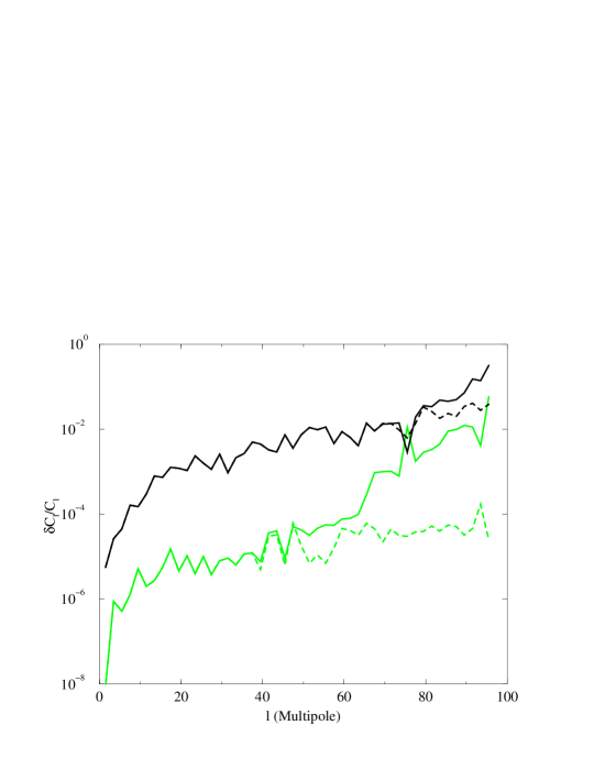
This graph demonstrates that there is much recoverable information available in the pixelized maps about modes up to $l\sim\sqrt{N_{tot}}$, at the cost of increased computational effort. However, we have performed this inversion using a very simple scheme, and there may well be more efficient ways of recovering it. In particular it may be worthwhile to consider using two pixelizations in which the ‘poles’ lie along orthogonal directions. The underlying $a_{lm}$’s which were hardest to recover from one pixelization would be very different from those which were hardest to recover from the other. So replacing the function $f$ in (17) by the sum of the two functions $f$ for each pixelization would likely remove some of the flat directions.

V Conclusions

We have shown that simple igloo pixelizations have much to commend them. They can easily be made hierarchical with pixels that are quite uniform. More importantly, they are naturally azimuthal, which speeds the calculation of spherical harmonics and allows for the exact calculation of the effect of the pixel shape. Including the effects of the pixel shapes is essential for the accurate extraction of the power spectrum without greatly over sampling the sky, and for understanding the systematic errors which can arise.

We should emphasize that in the limit of an infinite number of pixels, all the pixelizations are equivalent. In practice, the beam will be oversampled, which will help reduce the effects of pixelization for the multipoles of greatest interest. However, computational pressure will drive the number of pixels down, and remnants of the pixelization will exist to some degree. Igloo pixelizations provide an exact way of correcting for them.

In deciding what particular pixelization to use, a tradeoff must be made between the simplicity inherent in having few base pixels and the advantages of having pixels with the smallest amount of distortion possible. We have shown that having many base pixels has advantages in making the spherical harmonic representations on the pixelizations orthogonal, which minimizes errors in extracting power spectra. However, these factors must be weighed against the practical advantages having a simple and hierarchical scheme.

Of the models we have considered here, perhaps the best compromise between these considerations is the 3:6:3 equal latitude model. It has only twelve base pixels and can easily be created from an ECP pixelization. While it is only approximately equal area, we have found that this is actually an advantage because it allows us to prevent the average pixels from becoming more distorted. If exactly equal area models are favored, these can also be implemented using a 3:6:3 base igloo model.

Finally, we emphasize that there are many issues which we have not addressed here. For simplicity, we have assumed full sky coverage, though in practice the galaxy foreground will have to be removed. We also have focused on an ideal situation with no experimental noise, while realistically this will be large and will vary across the sky. These issues are crucial to eventually understanding the microwave background, but we have put them aside here to isolate the effects that arise from the process of the pixelization alone.

We wish to thank Richard Battye, Kris Gorski, Steven Gratton, David Spergel and Ned Wright for useful conversations, as well as members of the Cambridge Planck Analysis Center. R.C. acknowledges support from a PPARC Advanced Fellowship.

A Fast Integration of Legendre Polynomials

In calculating the true window function of a particular pixelization, it is useful to have an algorithm for the quick calculation of $\int P_{l}^{m}dx$ and its normalized counterpart, $\int\lambda_{l}^{m}dx.$ Just as for the calculation of the $P_{l}^{m}$’s themselves, they can be calculated by means of a recurrence relation.

Two of the recurrence relations that hold for the Associated Legendre polynomials are [11]

$$(1-x^{2}){dP_{l}^{m}(x)\over dx} = (l+1)xP_{l}^{m}(x)-(l-m+1)P_{l+1}^{m}(x),$$ (A1)

$$(2l+1)xP_{l}^{m}(x) = (l-m+1)P_{l+1}^{m}(x)+(l+m)P_{l-1}^{m}(x).$$ (A2)

Numerically, equation (A2) is generally used recursively to evaluate the Legendre polynomials, beginning with $P_{m}^{m}(x)$ and $P_{m+1}^{m}(x)$ [10].

Integrating the first relation, one finds

$$(1-x^{2})P_{l}^{m}(x)=(l-1)\int xP_{l}^{m}(x)dx-(l-m+1)\int P_{l+1}^{m}(x)dx.$$ (A3)

Now substituting in the second relation, we find the recursion relation for the Legendre polynomials

$$\int P_{l+1}^{m}(x)dx={(l-1)\over(l+2)}{(l+m)\over(l-m+1)}\int P_{l-1}^{m}(x)dx-{2l+1\over(l+2)(l-m+1)}(1-x^{2})P_{l}^{m}(x).$$ (A4)

In terms of the normalized polynomials, the recursion relation is,

$$\int\lambda_{l+1}^{m}(x)dx=\left({2l+3\over(l+m+1)(l-m+1)}\right)^{1/2}{1\over l+2}\left({(l-1)(l^{2}-m^{2})^{1/2}\over(2l-1)^{1/2}}\int\lambda_{l-1}^{m}(x)dx-(2l+1)^{1/2}(1-x^{2})\lambda_{l}^{m}(x)\right).$$ (A5)

This recursion requires the initial values, $\int\lambda_{m}^{m}(x)dx$ and $\int\lambda_{m+1}^{m}(x)dx$. The first of these can be found recursively, working up from $m=0,1$. However, this recursion becomes unstable when $\sin^{m}(\theta)$ is very small. When this is the case, one can rewrite the recursion as an expansion in powers of $1/m\cos^{2}\theta$, which quickly converges.

The second integral is given simply by the identity, $\int\lambda_{m+1}^{m}(x)dx=-(1-x^{2})\lambda_{m}^{m}(2m+3)^{1/2}/(m+2)$. To avoid round-off error, we perform the recursion for the integrals over the range of interest $\int^{x_{1}}_{x_{2}}\lambda_{l}^{m}(x)dx$, rather than doing them separately and taking the difference (i.e. $\int^{x_{1}}_{0}\lambda_{l}^{m}(x)dx-\int^{x_{2}}_{0}\lambda_{l}^{m}(x)dx$.)

B Pixelization as a Projection Operator

Pixelization projects the sky, which has infinite degrees of freedom parameterized by its $a_{lm}$’s, into a subspace of $N_{tot}$ dimensions, parameterized by the pixel temperatures, $T_{P}$. Thus, one can think of the operation which takes the true map to the pixelized map as a projection operator.

In real space this is self evident – pixelization projects the multi-dimensional temperature map over a pixel into a one dimensional space parameterized by its averaged temperature. In multipole space, this interpretation is less obvious. From equation (16), we can define the projection operator in multipole space to be

$${\cal P}_{lml^{\prime}m^{\prime}}\equiv\sum_{P}A_{P}W^{P}_{lm}W^{P*}_{l^{\prime}m^{\prime}}$$ (B1)

so that

$${\cal P}_{lml^{\prime}m^{\prime}}a_{lm}=a_{l^{\prime}m^{\prime}}^{pix}$$ (B2)

where the repeated indices are summed over.

Projection operators have the property that ${\cal P}^{2}={\cal P}$. One can show this for the operator defined above using the completeness of the spherical harmonics:

$$\sum_{lm}Y_{lm}(\Omega)Y^{*}_{lm}(\Omega^{\prime})=\delta(\Omega-\Omega^{\prime}).$$ (B3)

Multiplying both sides by $W^{P}(\Omega)W^{Q}(\Omega^{\prime})$ and integrating over both solid angles, one finds the pixelized analog

$$\sum_{lm}W^{P}_{lm}W^{Q*}_{lm}={1\over A_{P}}\delta_{PQ}.$$ (B4)

Thus,

$${\cal P}_{lml^{\prime}m^{\prime}}{\cal P}_{l^{\prime}m^{\prime}l^{\prime\prime}m^{\prime\prime}} = \sum_{P}A_{P}W^{P}_{lm}W^{P*}_{l^{\prime}m^{\prime}}\sum_{Q}A_{Q}W^{Q}_{l^{\prime}m^{\prime}}W^{Q*}_{l^{\prime\prime}m^{\prime\prime}}$$ (B5)

$$= \sum_{P}A_{P}W^{P}_{lm}\sum_{Q}A_{Q}W^{Q*}_{l^{\prime\prime}m^{\prime\prime}}{1\over A_{P}}\delta_{PQ}$$ (B6)

$$= \sum_{P}A_{P}W^{P}_{lm}W^{P*}_{l^{\prime\prime}m^{\prime\prime}}={\cal P}_{lml^{\prime\prime}m^{\prime\prime}}$$ (B7)

In real space, this is equivalent to saying that pixelizing a map that has already been pixelized yields the same map.

REFERENCES

- [1] For example, see E. B. Saff and A. B. J. Kuijlaars, The Mathematical Intelligencer, 19, 1, p5 (1997)
- [2] E. W. Greisen and M. Calabretta, Bull. American Astron. Soc., 182, 09.01 (1993) and references therein
- [3] J. R. Driscoll and D. M. Healy, Advances in Applied Mathematics, 15, 202 (1994)
- [4] M. J. Mohlenkamp, ‘A Fast Transform for Spherical Harmonics,’ Yale Thesis (1997)
- [5] P. F. Muciaccia, P. Natoli, N. Vittorio, Ap. J. Lett. 488, L63 (1997)
- [6] M. Tegmark, Ap. J. Lett., 470, L81 (1996)
- [7] R. Battye, private communication. See also P.W. Fowler and D.E. Manolopoulos, An Atlas of Fullerenes, New York: Oxford University Press, (1994)
- [8] K. Gorski, private communication (1997)
- [9] S. P. Oh, D. N. Spergel and G. Hinshaw, astro-ph/9805339 (1998)
- [10] W. H. Press, S. A. Teukolsky, W. T. Vettering and B. P. Flannery, Numerical Recipes, Second Ed., Cambridge: Cambridge University Press, (1992)
- [11] I. S. Gradshteyn and I. M. Ryzhik, Table of Integrals, Series and Products, New York: Academic Press, (1980)