The $L_{X}-T$ Relation and Intracluster Gas Fractions of X–ray Clusters

Abstract

We re-examine the X–ray luminosity–temperature relation using a nearly homogeneous data set of 24 clusters selected for statistically accurate temperature measurements and absence of strong cooling flows. The data exhibit a remarkably tight power–law relation between bolometric luminosity and temperature with a slope $2.88\pm 0.15$. With reasonable assumptions regarding cluster structure, we infer an upper limit on fractional variations in the intracluster gas fraction $\langle(\delta\hbox{$f_{gas}$}/\hbox{$f_{gas}$})^{2}\rangle^{1/2}\leq 15\%$. A strictly homogeneous GINGA subset of 18 clusters places a more stringent limit of $9\%$.

Imaging data from the literature are employed to determine absolute values of $f_{gas}$ within spheres encompassing density contrasts $\delta_{c}\!=\!500$ and 200 with respect to the critical density. Comparing binding mass estimates based on the virial theorem (VT) and the hydrostatic, $\beta$–model (BM), we find a temperature–dependent discrepancy in $f_{gas}$ between the two methods caused by systematic variation of the outer slope parameter $\beta$ with temperature. Mean values (for ${\rm\ H_{o}}\!=\!50{\rm\ km\ s^{-1}\ Mpc^{-1}}$) range from $\hbox{${\bar{f}}_{gas}$}\!=\!0.10$ for cool ($T<4{\rm\ keV}$) clusters using the VT at $\hbox{$\delta_{c}$}\!=\!500$ to $0.22$ for hot ($T>4{\rm\ keV}$) clusters using the BM at $\hbox{$\delta_{c}$}\!=\!200$. There is evidence that cool clusters have a lower mean gas fraction than hot clusters, but it is not possible to assess the statistical significance of this effect in the present dataset. The $T$ dependence of the ICM density structure, coupled with the increase of the gas fraction with $T$ in the VT approach, explains the steepening of the $L_{X}$–$T$ relation.

The small variation about the mean gas fraction within this majority sub–population of clusters presents an important constraint for theories of galaxy formation and supports arguments against an Einstein–deSitter universe based on the population mean gas fraction and conventional, primordial nucleosynthesis. The apparent trend of lower gas fractions and more extended atmospheres in low temperature systems are consistent with expectations of models incorporating the effects of galactic winds on the intracluster medium.

1 Introduction

The relation between X–ray temperature $T$ and luminosity $L_{X}$ is a sensitive diagnostic of structural regularity in clusters of galaxies. Because the luminosity is governed by the mass of gas in the intracluster medium (ICM) while the temperature is determined by the total, gravitating cluster mass, the $L_{X}$–$T$ relation can be used as a tool to probe variations in gas fraction — the ratio of ICM gas to total mass — in these systems.

Evidence for a correlation between these basic observational quantities has existed since the early days of X–ray astronomy (Mitchell et al. 1977, 1979; Mushotzky et al. 1978; Edge & Stewart 1991, David et al. 1993). Despite its relative maturity, a key characteristic of this relation was only recently established. Fabian et al. (1994) demonstrate that the departure of a cluster from the mean $L_{X}-T$ relation is correlated with the strength of the emission associated with its cooling flow core. The picture resulting from this work is of a mixed population which is likely to be time variable. Fabian et al. speculate that cooling flows are a recurrent phenomenon associated with a secular instability in the ICM plasma which periodically is interrupted and reset by strong merging encounters. Periodic mergers of varying strength are a natural feature of hierarchical clustering models of structure formation, and numerical simulations suggest that cooling flow features can be erased by mergers (Garasi, Burns & Loken 1997). However, the theoretical picture remains incomplete because of the complexities of the physics operating in the cluster core. Regardless of the exact physical mechanisms responsible, the empirical fact is that the cluster population can be broadly classed into two categories by making a cut in cooling flow strength $\dot{M}$.

In this paper, we present and analyze the luminosity–temperature relation from a nearly homogeneous data set of weak cooling flow clusters, where $\hbox{$\dot{M}$}\leq 100{\rm\ M}_{\odot}{\rm\ yr}^{-1}$ defines weak. The data set is described in §2, with particular attention paid to systematic errors in determination of both $L_{X}$ and $T$. In §3, we present the $L_{X}$–$T$ relation and show that these data place stringent limits on gas fraction variations within this sub–population. Imaging data taken from the literature allow us to estimate absolute values of the gas fraction at fixed density contrast in §4. We compare results for two different binding mass estimation methods, and emphasize the systematic uncertainty introduced by this choice.

Hubble constant dependencies are displayed in the paper via $\hbox{$\,h_{50}$}\equiv{\rm\ H_{o}}/50{\rm\ km\ s^{-1}\ Mpc^{-1}}$ and we assume $\hbox{$\,h_{50}$}\!=\!1$ when quoting numerical values throughout the paper.

2 The Sample

We analyse an archival data set, part of which was assembled and discussed by Arnaud (1994). A prime objective is to limit both statistical and systematic errors in $L_{x}$ and $T$, in order to obtain an accurate assessment of the intrinsic dispersion about the mean $L_{X}-T$ relation.

Table 1: Basic data for the 24 clusters in the sample

Name	Redshift	$L_{\rm X}$ [2-10 keV]	Temperature	Abund.	$L_{\rm bolom.}$	$\beta$	Core radius	Ref.
		(ergs/s)	(keV)	(rel. solar)	(ergs/s)		(kpc)
Virgo	0.0038	$2.00~{}10^{43}$	$2.20\pm 0.02$	0.44	$6.81~{}10^{43}$	0.46	12.6	29,29,7,7
A262	0.0164	$3.70~{}10^{43}$	$2.41\pm 0.05$	0.55	$1.15~{}10^{44}$	$0.53\pm 0.03$	$95\pm 25$	34,34,12,19
A644	0.0704	$1.06~{}10^{45}$	$6.59\pm 0.17$	0.33	$2.24~{}10^{45}$	0.70	204	16,16,20,20
A754	0.0534	$1.16~{}10^{45}$	$7.57\pm 0.31$	0.23	$2.46~{}10^{45}$	-	-	1,1
A1367	0.0215	$9.09~{}10^{43}$	$3.50\pm 0.18$	0.31	$2.26~{}10^{44}$	$0.50\pm 0.10$	$390_{-130}^{+210}$	16,16,29,20
A1656	0.0232	$1.13~{}10^{45}$	$8.21\pm 0.09$	0.22	$2.41~{}10^{45}$	$0.75\pm 0.03$	$420\pm 24$	18,18,8,8
A2256	0.0601	$1.11~{}10^{45}$	$7.51\pm 0.19$	0.28	$2.35~{}10^{45}$	$0.81\pm 0.01$	$542\pm 12$	16,16,9,9
A2319	0.0564	$2.24~{}10^{45}$	$9.12\pm 0.15$	0.24	$4.83~{}10^{45}$	$0.68\pm 0.05$	$410\pm 50$	34,34,19,19
A2634	0.0321	$7.09~{}10^{43}$	$3.07\pm 0.11$	0.38	$1.89~{}10^{44}$	0.58	320	1,1,11,11
A3526	0.0109	$7.00~{}10^{43}$	$3.54\pm 0.13$	0.54	$1.70~{}10^{44}$	$0.45\pm 0.03$	$93\pm 19$	32,33,23,23
A3921	0.0940	$5.20~{}10^{44}$	$4.90\pm 0.55$	0.26	$1.15~{}10^{45}$	$0.75\pm 0.04$	$385\pm 42$	2,2,2,2
AWM4	0.0315	$2.53~{}10^{43}$	$2.43\pm 0.28$	0.93	$7.52~{}10^{43}$	0.43	190	31,31,31,31
AWM7	0.0179	$1.70~{}10^{44}$	$3.82\pm 0.15$	0.49	$3.99~{}10^{44}$	$0.53\pm 0.01$	$102\pm 5$	31,31,28,28
Ophui.	0.0280	$1.90~{}10^{45}$	$9.10\pm 0.30$	0.24	$4.10~{}10^{45}$	$0.62^{+0.01}_{-0.02}$	$177^{+46}_{-93}$	21,21,24,24
A665	0.1820	$1.50~{}10^{45}$	$8.26\pm 0.90$	0.49	$3.16~{}10^{45}$	$0.66\pm 0.05$	$379\pm 70$	17,17,5,5
A1413	0.1427	$1.82~{}10^{45}$	$8.85\pm 0.50$	0.19	$3.92~{}10^{45}$	0.62	156	16,16,11,11
A2163	0.2010	$6.00~{}10^{45}$	$14.6\pm 0.85$	0.40	$1.45~{}10^{46}$	$0.62\pm 0.02$	$305\pm 19$	14,14,14,14
A2218	0.1710	$9.40~{}10^{44}$	$6.70\pm 0.50$	0.20	$2.00~{}10^{45}$	$0.65^{+0.08}_{-0.05}$	$226^{+80}_{-50}$	25,25,6,6
A370	0.3700	$1.30~{}10^{45}$ [1]	$8.80\pm 0.80$	0.50	$2.76~{}10^{45}$	-	-	4,4
A399	0.0715	$7.76~{}10^{44}$ [3]	$7.40\pm 0.50$	0.25	$1.64~{}10^{45}$	$0.52\pm 0.05$	$215\pm 35$	13,15,19,19
A401	0.0748	$1.47~{}10^{45}$ [3]	$8.40\pm 0.50$	0.21	$3.15~{}10^{45}$	$0.61\pm 0.01$	$285\pm 10$	13,15,19,19
A1060	0.0114	$2.50~{}10^{43}$ [2]	$3.10\pm 0.20$	0.40	$6.60~{}10^{43}$	0.61	94.	13,30,22,22
A3558	0.0478	$4.23~{}10^{44}$ [2]	$5.50\pm 0.25$	-	$9.06~{}10^{44}$	0.61	324	13,27,3,3
Trian.	0.0510	$1.26~{}10^{45}$ [2]	$10.3\pm 0.80$	0.26	$2.77~{}10^{45}$	$0.63\pm 0.02$	$286\pm 16$	13,26,26,26

Notes: column (9) references for the data (respectively X–ray luminosity, temperature , $\beta$ and core radius): 1. Arnaud (1994); 2. Arnaud et al. (1997); 3. Bardelli et al. (1996); 4. Bautz et al. (1994); 5. Birkinshaw, Hughes & Arnaud (1991); 6. Birkinshaw & Hughes (1994); 7. Böhringer et al. (1994); 8. Briel, Henry & Böhringer (1992); 9. Briel & Henry (1994); 10. Buote & Canizares (1996); 11. Cirimele, Nesci & Trevese (1997); 12. David, Jones & Forman (1995); 13. Edge et al. (1990); 14. Elbaz, Arnaud & Böhringer (1995); 15. Fujita et al. (1996); 16. Hatsukade (1989); 17. Hughes & Tanaka (1992); 18. Hughes et al. (1993); 19. Jones & Forman (1984); 20. Jones & Forman (1990, priv. comm.); 21. Kafuku et al. (1992); 22. Loewenstein & Mushotzky (1996); 23. Matilsky, Jones & Forman (1985); 24. Matsuzawa et al. (1996); 25. McHardy et al. (1990); 26. Markevitch, Sarazin & Irwin (1996); 27. Markevitch & Vikhlinin (1997); 28. Neumann & Böhringer (1995); 29. Takano (1990) and Koyama (1997, priv. comm.); 30. Tamara et al. (1996); 31. Tsuru (1993); 32. Yamanaka & Fukazawa (priv. comm. in Fukazawa et al. (1994)); 33. Yamashita 1992; 34. Yamashita (1997, priv. comm.)

2.1 Selection Criteria

Inclusion of a cluster in the sample is based on three criteria : (i) small statistical errors in measured temperature $\Delta T/T\!\mathrel{\hbox to0.0pt{\lower 3.0pt\hbox{$\mathchar 536\relax$}\hss}\raise 2.0pt\hbox{$\mathchar 316\relax$}}\!10\%$ (at $90\%$ confidence), (ii) weak or absent cooling flow $\hbox{$\dot{M}$}\!\leq\!100{\rm\ M}_{\odot}{\rm\ yr}^{-1}$, and (iii) $kT\geq 2{\rm\ keV}$. The value of $\dot{M}$ is set by the relative importance of core luminosity to the total, and is typically evaluated using models of multi–phase, steady–state accretion (Thomas, Fabian & Nulsen 1987). Since nearly two–thirds (33/51) of the clusters in the X–ray flux limited sample of Edge et al. (1990) have flows below this limit (Fabian et al. 1994), our analysis is of a majority population.

Table 1 presents a listing of the 24 clusters satisfying the above criteria. Eighteen have both $T$ and $L_{X}$ determined by the GINGA satellite (references are given in the table). Luminosities for three nearby clusters (Virgo, in particular) are calculated from scanning data, which accounts directly for the extended emission outside the $1.1\times 2$ sq deg FOV (FWHM) of the satellite instrument. Temperature measurements for the other six clusters come from ASCA, with luminosities from Einstein MPC (3), EXOSAT (2), and ASCA (1).

We believe this list to be complete with respect to publications available end of 1996. Sixteen clusters in our sample are included in the X-ray flux limited sample of Edge et al. (1990). Two more clusters (A2163 and A1413) have fluxes above the Edge et al flux limit ($1.7\times 10^{-11}{\rm\ erg\ s^{-1}\ cm^{-2}}$). Our sample is $\sim 70\%$ complete as compared to the Edge et al. sample down to a flux of $3.4\times 10^{-11}{\rm\ erg\ s^{-1}\ cm^{-2}}$ (considering from now on only weak cooling flow clusters in the Edge sample for consistency) and highly incomplete below this flux (3 clusters among 20). The other clusters of our sample below the Edge et al. flux limit are either distant luminous clusters (A3921, A665, A2218, A370) or poor clusters (A2634 and AWM4). The temperature distribution of our sample shows a clear deficit of clusters at intermediate temperature ($4-6$ keV) as compared to the temperature distribution of the Edge et al. sample.

Included in Table 1 are the measured temperature and luminosity in the 2–10 keV energy band (cluster rest frame and corrected for absorption). We convert the 2–10 keV luminosity to bolometric luminosities using an isothermal plasma emission model (Mewe, Gronenshild & van den Oord 1985; Mewe, Lemen & van den Oord 1986) and the measured temperatures and abundances. The bolometric correction factor depends mostly on the temperature; it is higher at low temperature ($\sim 3.4$ at 2.2 keV), decreases with increasing temperature up to about 8 keV ($\sim 2.1$) and increases again above ($\sim 2.4$ at 15 keV). The statistical errors on the luminosities are always much smaller than the corresponding errors on the temperature and are thus not taken into account here.

2.2 Systematic Errors

To estimate accurately the intrinsic dispersion of the $L_{X}-T$ relation requires an attempt to understand and quantify sources of systematic errors. Such errors can arise from calibration uncertainties, systematic errors in background subtraction and, for luminosities deduced from collimated instruments (EXOSAT, GINGA), improper correction for cluster extent (loss of efficiency at large radii, emission outside the FOV). Further uncertainties due to the uncertainties on the plasma emission model are negligible for clusters in the considered temperature range (see Arnaud et al. 1991; Arnaud et al. 1992).

We attempt to guage the magnitude of systematic uncertainty in the bolometric luminosity by comparing to values derived from the ROSAT All–Sky Survey (RASS) by Ebeling et al.  (1996) for Abell Clusters. Eigthteen of the clusters in our sample are in this dataset. We convert the RASS band–limited, total unabsorbed flux, derived from a procedure described in the above reference, to bolometric $L_{X}$ using the same plasma emission model as that used on our own data. In addition, we include RASS data for Virgo from Böhringer et al.  (1994) and ROSAT imaging data for Triangulum (Markevitch, Sarazin & Irwin, 1996) and Ophiuchus (Buote & Tsai 1996), from which we calculate total luminosities by extrapolating the $\beta$–model fits given in the references. Conversion to a bolometric measure for imaging data is the same as for the RASS data.

We find good agreement between the GINGA and ROSAT bolometric luminosities; 16 objects yield a mean ratio of $1.00$ with standard deviation of $0.19$. The agreement is not as good for the five non–GINGA members of our sample, but the difference is driven entirely by two clusters — Triangulum and A3558 — for which the ROSAT luminosities are larger than the EXOSAT values we use by factors of $1.72$ and $1.56$, respectively. Both clusters are nearby and have extent comparable or larger than the EXOSAT FOV ($45^{\prime}\times 45^{\prime}$ FWHM), the virial radius (defined below) of these 2 clusters are respectively at 49 and 38 arcmin from the center. Their flux can be underestimated due to the neglect of the loss of efficiency at large radii. Furthermore, both observations were significantly offset, the pointing offset being specially important for A3558 (38 arcmin, Edge 1989). Although the fluxes published by Edge et al. (1990) include correction for this effect (correction as for a point source), this is likely to induce further uncertainties in the flux estimate. For the sake of consistency with the remaining dataset, we applied no correction to the published values.

The comparison of the GINGA and ROSAT luminosities, which constitutes the majority of our sample, indicates that the scatter expected from systematic uncertainty in $L_{X}$ is not larger than $20\%$ (rms). Clusters with large angular extent — in particular, larger than GINGA’s $1.1\deg\times 2\deg$ field of view — are likely to incur larger error, but the number of such objects in our sample is small. Furthermore, we looked for systematic variation with redshift of the ratio between the GINGA and ROSAT luminosities. Such a dependence with redshift was noticed by Ebeling (1993) for the ratio between the luminosities (HEAO, MPC and EXOSAT data) given by Henry & Arnaud (1991) and the RASS luminosities. The observed increase of this ratio with redshift (up to $z\sim 0.07$) was interpreted as being due to an underestimate of flux for nearby, extended clusters by earlier experiments. This effect is not apparent in the GINGA data, due to the larger instrument FOV and the use of scanning mode for the most extended clusters.

We now consider systematic errors on temperature. A detailed estimate of this error, due to calibration uncertainties and background subtraction, was done by Hughes et al. (1993) for the GINGA observation of Coma. They found a systematic uncertainty of $\pm 0.13$ keV which, in fact, dominates the especially small statistical uncertainty ($\pm 0.09{\rm\ keV}$) for this cluster. Arnaud et al. (1992) also found a typical systematic uncertainty due to background subtraction of $0.14$ keV for A2163 ($T\!=\!14.5$ keV). Although this systematic error is expected to depend on cluster flux and temperature, these typical figures show that, for most of the clusters considered here, statistical errors still dominate the systematic errors. This is further confirmed if one compares the temperature estimates from various instruments. Generally, good agreement between MPC, EXOSAT and GINGA estimates is found (David et al. 1993), as well as between ASCA and other high-energy instruments (Markevitch & Vikhlinin 1997). A direct comparison between the temperature estimate for the 7 clusters in our sample with both GINGA and EXOSAT measurements gives a mean ratio of $0.97$ with standard deviation of $0.06$.

3 The $L_{X}-T$ Relation and Implications

3.1 The $L_{X}-T$ Relation

Figure 1 shows the luminosity–temperature relation for the sample, with $90\%$ confidence errors plotted for $T$. Statistical errors on $L_{X}$ are typically smaller than the plotted point size and so are not shown. The homogeneous GINGA sample data are shown as filled circles, the remainder as open circles. The set of clusters define a remarkably tight relation. The main outliers are A1060 and Triangulum, which are anomalously dim (or hot) in comparison to the others. The deviation of Triangulum is significantly reduced if the ROSAT luminosity is employed in place of the EXOSAT value. As noted above, this difference is likely due to its large angular extent. The peculiarity of A1060 was noted by Loewenstein & Mushotzky (1996) in a direct comparison to AWM7, a cluster of similar temperature which is also in our sample. Girardi et al. (1997) also pointed out the departure of this cluster from the general $L_{X}-T$ relation. They noted that its temperature is high compared to its velocity dispersion and suggested some anomalies in the dynamical state of the gas. However they assumed a temperature of 3.9 keV from David et al (1993), which is significantly higher than the more precise ASCA value adopted here. From the velocity dispersion, $\sigma=633$km/s, determined by Girardi et al. (1997) and the best fit $\sigma-T$ relation established by Girardi et al. (1996), we actually expect a temperature of 2.8 keV, in reasonable agreement with the ASCA value of $3.1\pm 0.2$ keV. The deviation of A1060 is only sligtly decreased if this value is used instead of the ASCA value. Either both the galaxies and the gas are in a very particular dynamical state or the gas structure or content in this cluster is abnormal.

Figure 1: The luminosity—temperature relation for the 24 clusters used in this analysis. Filled circles are the homogeneous GINGA subset while open circles denote clusters with ASCA temperatures and EXOSAT, MPC, or ASCA luminosities. Error bars plotted on $T$ are $90\%$ confidence limits. The solid line is the best–fit relation; the dashed lines are offset by an amount equal to the rms deviation in log$(L_{X})$ about the mean relation. The upper insert shows a histogram of the luminosity residuals (in dex), which makes apparent the two principal outliers, A1060 and Triangulum.

The data are well fit by a power law $\hbox{log$(L_{X})$}=(2.88\pm 0.15)\hbox{log$(T/6{\rm\ keV})$}+(45.06\pm 0.03)$. The central values and uncertainties in the fit parameters are derived from simple least squares fits (in log space) to a large number of bootstrap resamplings employing the estimated $T$ measurement errors (quoted errors in slope and intercept are $1\sigma$). Note that since bootstrap procedure is used to estimate errors the exact fit method is of secondary importance. The slope of $2.88\pm 0.15$ is consistent with that found by Ebeling (1993) from RASS luminosities ($2.73\pm 0.39$) but is significantly smaller than the value of 3.36 found by David et al. (1993) using mostly MPC and EXOSAT data. This is a direct consequence of the underestimate of luminosities for nearby clusters by these last two experiments (see above); the observed clusters with low luminosities being on average at smaller distance than more luminous clusters which can be observed up to larger distances. Our slope is also consistent at better than the $2\sigma$ level with the recent value of $2.64\pm 0.16$ determined by Markevitch (1998) from analysis of ASCA temperatures and ROSAT luminosities of nearby clusters. Allen & Fabian (1998) find a slope of $2.9\pm 0.3$ in the non cooling flow portion of their combined ASCA/ROSAT sample.

The raw scatter in decimal log$(L_{X})$ about the luminosity–temperature relation is $0.14$, and some of the variance arises from measurement errors in temperature. We estimate this contribution to be $0.06$, and thus calculate the intrinsic scatter in log$(L_{X})$ at fixed temperature to be $0.13$, equivalent to a fractional deviation $\langle(\delta L_{X}/L_{X})^{2}\rangle^{1/2}\!=\!0.30$. For the homogeneous GINGA subset of 18 clusters, the fractional deviation reduces substantially, to $0.17$.

Considering A1060 as an outlier, the fact that there is no significant trend toward larger scatter in $L_{X}$ at low temperatures implies that cooling flows do not contribute substantially to the total luminosity of these systems. Our selection criterion of a fixed cooling flow mass deposition rate is roughly equivalent to an absolute limit in core luminosity excess attributed to the cooling flow region. This absolute limit represents a larger fraction of the total luminosity from smaller systems, leading to the concern that cooling flows of variable strength (but under our $100{\rm\ M}_{\odot}{\rm\ yr}^{-1}$ limit) might induce larger variance at low temperatures if the cooling region dominated the luminosity. This effect is not apparent in this data set of modest number.

3.2 Limits on Gas Fraction Variations

The small scatter in Figure 1 supports the notion that at least this sub–population of weak cooling flow clusters is quite regular in its structural properties. In particular, the data appear at odds with the idea of large gas fraction variations within the virial regions of clusters, an idea hinted at by the comparison of A1060 to AWM7 by Loewenstein & Mushotzky (1996). We now address this issue using a spherically symmetric model as a framework for calculation. The purpose of the exercise is to provide a context for connecting the scatter in gas fraction at fixed temperature with the observed variance in X–ray luminosity. The exercise is non-trivial because luminosity scatter can be due to changes in gas density structure as well as overall gas fraction variations.

Consider a cluster with smooth, spherically symmetric distributions of gas and total mass about its center. Let $M_{\delta_{c}}$ be the total mass contained in a sphere (of radius $r_{\delta_{c}}$ about the center) which encompasses a mean density $\delta_{c}\hbox{$\rho_{c}$}$, where $\hbox{$\rho_{c}$}\equiv 3{\rm\ H_{o}}^{2}/8\pi G$ is the critical density of the universe within which the cluster is embedded. The bolometric X–ray luminosity of a cluster is

$$L_{X}\ =\ \int d^{3}r\ \rho_{gas}^{2}(r)\ \Lambda(T(r))$$ (1)

where $\Lambda(T(r))$ is an appropriately normalized emissivity dependent only on temperature. In practice, the integral extends not to infinity, but to a finite radius denoting the edge of the relaxed, virialized portion cluster. Spherical collapse models and numerical simulations suggest that this edge is located at density contrast $\delta_{c}\!\simeq\!200$, or radius $r_{200}$.

Writing the gas density in terms of the natural radial variable $y\!\equiv\!r/\hbox{$r_{\delta_{c}}$}$, we introduce the structure function $h(y)$

$$\rho_{gas}(y\hbox{$r_{\delta_{c}}$})\ \equiv\ f_{gas}\ \hbox{$\delta_{c}$}\,\hbox{$\rho_{c}$}\ h(y),$$ (2)

where the explicit use of the gas fraction within density contrast $\delta_{c}$

$$\hbox{$f_{gas}$}\ \equiv\ \frac{M_{gas}(<\hbox{$r_{\delta_{c}}$})}{\hbox{$M_{\delta_{c}}$}}$$ (3)

sets the normalization of the structure function $h(y)$ via the condition $3\int_{0}^{1}dyy^{2}h(y)\!=\!1$ . For an ensemble of clusters, we imagine a set of gas fraction values $\{\hbox{$f_{gas}$}\}$ and structure functions $\{h(y)\}$.

The luminosity in equation (1) with this notation becomes

$$L_{X}\ \equiv\ \hbox{$f_{gas}$}^{2}\ Q(\hbox{$\delta_{c}$},T)$$ (4)

where

$$Q(\hbox{$\delta_{c}$},T)\ =\ \int d^{3}y\ h^{2}(y)\ [\Lambda(T(y))\hbox{$\rho_{c}$}^{2}\hbox{$\delta_{c}$}^{2}\hbox{$r_{\delta_{c}}$}^{3}]$$ (5)

is largely determined by the structure function $h(y)$, with weaker dependence on the form of the temperature distribution through $T(y)$.

The variance in luminosity at fixed temperature has contributions from gas fraction variations and structural variations

$$\delta_{L}^{2}\ =\ 4\delta_{f}^{2}+4\delta_{f}\delta_{Q}+\delta_{Q}^{2},$$ (6)

where the $\delta$’s are fractional variations at fixed temperature

$$\delta_{L}\equiv\biggl{(}\frac{\delta L_{X}}{L_{X}}\biggr{)}_{T}\ ,\ \delta_{f}\equiv\biggl{(}\frac{\delta\hbox{$f_{gas}$}}{\hbox{$f_{gas}$}}\biggr{)}_{T}\ ,\ \delta_{Q}\equiv\biggl{(}\frac{\delta Q}{Q}\biggr{)}_{T}.$$ (7)

The magnitude of intracluster gas variations $\delta_{f}$ can be determined from the observed scatter in luminosity $\delta_{L}$

$$\delta_{f}^{2}\ =\ \frac{1}{4}(\delta_{L}^{2}-\delta_{Q}^{2})-\delta_{f}\delta_{Q}$$ (8)

with an additional assumption about how changes in gas fraction and cluster structure are correlated. We assume here that there are no correlations between changes in gas content and variations in internal structure, meaning

$$\langle\delta_{f}\delta_{Q}\rangle\ =\ 0$$ (9)

with the angle brackets denoting an ensemble average.

With this assumption, the fact that $\delta_{Q}^{2}$ is positive definite leads to an upper limit on gas fraction variations from equation (6)

$$\langle\delta_{f}^{2}\rangle^{1/2}\ \leq\ \frac{1}{2}\ \langle\delta_{L}^{2}\rangle^{1/2}.$$ (10)

and the resultant values from Figure 1 are

$$\langle\delta_{f}^{2}\rangle^{1/2}\ \leq\ \cases{0.15&full sample,\cr 0.09&GINGA subsample.\cr}$$ (11)

Enlarging these limits is possible if an anti–correlation exists between $\delta_{f}$ and $\delta_{Q}$. Such an anti–correlation would require gas poor clusters to be more centrally concentrated than average, and vice–versa. In this way, the change in luminosity due to a lower (higher) gas mass would be compensated by an increased (decreased) central density. We show below that the observational data do not support such an anti–correlation. In addition, one mechanism capable of generating gas loss from clusters has the opposite effect. Heating due to winds from early–type galaxies leads to a less centrally concentrated ICM structure and slightly depressed gas fractions within the virial radius (Metzler & Evrard 1997). This implies $\langle\delta_{f}\delta_{Q}\rangle>0$, a result which serves to strengthen the limit imposed by equation (8).

We conclude that variations in gas fraction within the virial regions (overdensities $\hbox{$\delta_{c}$}\!\sim\!200$) of weak, cooling flow clusters are likely to be quite small. Fractional deviations at fixed temperature $\delta_{f}$ may have standard deviation smaller than $10\%$, particularly if galactic wind feedback, or some other, non–gravitational, entropy generating mechanism, has produced correlated variations in gas fraction and density structure.

The limit on gas fraction variations applies to clusters of similar temperature; there remains the possibility that the mean cluster gas fraction varies, perhaps considerably, over the range of temperatures probed in our sample.

4 Temperature Dependence of ICM Structure

In this section, we examine our sample for evidence of variation in the mean cluster ICM structure and virial gas fraction with cluster temperature. We also discuss the origin of the $L_{X}$–$T$ relation slope.

4.1 The slope of the $L_{X}$–$T$ relation

Suppose that cluster density profiles $h_{T}(y)$ and gas fractions $\hbox{$f_{gas}$}(T)$ are, in the mean, temperature dependent. If we further suppose that clusters are internally isothermal, then equation (4) can be rewritten in a form which makes clear the dependence on the shape function $h_{T}(y)$

$$L_{X}(T)\ =\ f_{gas}^{2}(T)\ [\hbox{$M_{\delta_{c}}$}(T)\hbox{$\rho_{c}$}\hbox{$\delta_{c}$}\Lambda(T)]\ \hat{Q}(T)$$ (12)

with $\hat{Q}(T)=(3/4\pi)\int d^{3}y\,h_{T}^{2}(y)$ is the dimensionless emission measure. Note that $\hat{Q}(T)$ is equal to $\langle{\rho_{gas}^{2}}\rangle/\langle{\rho_{gas}}\rangle^{2}$, with the angle brackets denoting the average over the cluster atmosphere. It is thus a structure factor which depends solely on the gas density shape and characterises the concentration of the gas distribution.

The traditional approach is to employ the following set of additional assumptions : (i) pure bremsstrahlung emission ($\Lambda(T)\!\propto\!T^{1/2}$), (ii) virial equilibrium ($\hbox{$M_{\delta_{c}}$}\!\propto\!T^{3/2}$), (iii) structurally identical clusters ($\hat{Q}(T)\!=\!C_{1}$), and (iv) constant gas fraction ($\hbox{$f_{gas}$}(T)\!=\!C_{2}$). This leads to an expected scaling relation between luminosity and temperature of slope two

$$L_{X}(T)\ \propto\ T^{2}.$$ (13)

The fact that the slope of the observed relation is significantly steeper than two implies that one or more of these assumptions does not hold in the real cluster population. For example, if we retain bremsstrahlung emission and the condition of virial equilibrium, then the observed slope of the $L_{X}$–$T$ relation leads to a constraint on structure factor and gas fraction dependence

$$\hbox{$f_{gas}$}^{2}(T)\hat{Q}(T)\ \propto\ T^{0.88\pm 0.15}.$$ (14)

The assumption of pure bremsstrahlung is quite accurate above about 2 keV, but at lower temperatures, line emission becomes significant unless the metallicity is very low. Pure bremsstrahlung emission itself does not exactly scales as $T^{1/2}$ due to the additional Gaunt factor. However, this factors varies by less than $4\%$ in the 1–10 keV temperature range. On the other hand, the line emission reaches about $18\%$ of the total emission at 2 keV for a typical abundance of 1/3 the solar value. This extra line emission tends to flatten the slope of the $L_{X}$–$T$ relation, as low $T$ clusters are boosted in luminosity more than their high $T$ counterparts. This effect is amplified because low $T$ clusters tend to have higher abundances. Given the measured abundances we computed $\Lambda(T)$ for our sample (the correct value is used in all the following). We found that the departure from the $T^{1/2}$ law is actually small: the best fit slope of the power law is 0.36 instead of 0.5.

The assumption of virial equilibrium is supported by cosmological, gasdynamic simulations (Bryan & Norman 1998 and references therein). The relation holds particularly well for $\hbox{$\delta_{c}$}\simeq 200-2500$, with 200 the fiducial choice of virial radius and 2500 approaching the onset of the cluster core. We use the virial theorem as one method for estimating total cluster masses below.

There remains the issue of structural regularity. Recent numerical investigation of dark matter halos evolved within hierarchical clustering cosmogonies indicates that low mass halos are, on average, more centrally concentrated than high mass halos (Navarro et al. 1997). Although the magnitude of the change is likely to be small within the mass range probed by the X–ray clusters in our sample, the qualitative direction is again to flatten the slope of the $L_{X}$–$T$ relation, if one assumes that the gas density follows that of the dark matter.

The assumption that the gas traces the dark matter is reasonable if shock heating through gravitational infall is the only entropy generating mechanism, but this assumption breaks down if extra energy sources or sinks are available to the gas. In particular, if galactic winds play an important role in heating the ICM, then the extra entropy dumped into the gas can change its density structure dramatically (Metzler & Evrard 1994). The net result of winds is to inflate the gas distribution, decreasing the $\hat{Q}$ factor and causing diminished gas densities and, correspondingly, lowered gas fractions, at radii interior to the virial radius. Because supernova–driven winds impart roughly a fixed specific energy into their surroundings, their impact is felt more strongly in shallower potential wells. This steepens and lowers the intercept of the $L_{X}$–$T$ relation compared to models without winds.

The magnitude of this effect will depend on details of the assumed wind model, but plausible models exist. The numerical simulations of Metzler (1994) produce a slope of $2.96\pm 0.05$ in the bolometric $L_{X}$–$T$ relation. Cavaliere, Menci & Tozzi (1997) create a semi–analytic model which predicts a progressive steepening of the $L_{X}$–$T$ slope toward low temperature clusters, consistent with the data of Ponman et al. (1996). Finally, the constant central entropy model of Evrard & Henry (1991) predicts a slope of $2.75$ which is consistent, within the errors, with our observational sample behaviour.

4.2 Gas density profiles from X–ray imaging

Azimuthally averaged profiles of cluster X–ray surface brightness images are generally well fit by the standard, $\beta$–model form

$$I(r)\ =\ I_{0}\,\left[1+(r/r_{c})^{2}\right]^{-3\beta+1/2}$$ (15)

derived by assuming an isothermal gas with density distribution $\rho_{gas}(r)=\rho_{0}(1+(r/r_{c})^{2})^{-3\beta/2}$. Fits to this model exist for all but two (A754 and A370) of the members of our sample. Table 1 lists values from the literature of the best–fit core radius $r_{c}$ and outer slope parameter $\beta$. Errors on these parameters are also given in the table when available.

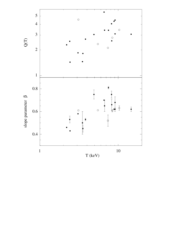
Figure 2: Values of the gas outer slope parameter $\beta$ (bottom) and structure factor $\hat{Q}$ (top), derived from $\beta$–model fits to X–ray images plotted against temperature for 22 of the 24 members of our sample. Point styles are the same as the previous figures. Error bars available in the literature are shown.

Figure 2 displays the best fit slope parameters against temperature. As noted previously (David et al. 1990; White 1991; Mohr & Evrard 1997), there is a clear trend toward decreasing $\beta$ toward lower $T$. This trend is not likely to be an artifact of the fitting procedure, as Mohr & Evrard (1997) see a similar trend with $\beta$ defined in a non–parametric, non–azimuthally averaged fashion.

The heterogeneous nature and lack of error estimates for nearly a third of these data make it difficult to determine the formal statistical significance of this effect. As a reasonable estimate, we calculate the bi–weight modes (Beers, Flynn & Gebhardt 1990) for the subsamples of 8 clusters with $T<4{\rm\ keV}$ and 14 clusters with $T>4{\rm\ keV}$. We applied a $10\%$ fractional error to each data point — slightly larger than the rms  fractional error of $7.8\%$ for the 15 quoted error values — and determined the expected subsample means and standard error from bootstrap analysis. The values of $\langle\beta\rangle_{lo}\!=\!0.51\pm 0.03$ and $\langle\beta\rangle_{hi}\!=\!0.66\pm 0.03$ for the low– and high–$T$ subsamples differ at the $3.3\sigma$ level. We suspect that future analysis with a more regular dataset will confirm the statistical significance of this trend.

The implication is that the ICM density structure of clusters is temperature dependent, and the sense of the effect is such that $\hat{Q}(T)$ is an increasing function of temperature (see Figure 2). Models of cluster formation incorporating galactic winds exhibit a trend of $\beta$ versus $T$ similar to that seen in the observational data (Metzler & Evrard 1997). The trend of $\hat{Q}(T)$ with temperature is in the right direction to steepen the $L_{X}$–$T$ relation, but whether it is entirely responsible for this effect requires investigation of the trend of mean gas fraction with temperature.

4.3 Intracluster Gas Fraction Values

The determination of absolute values of the gas fraction requires a method to estimate the total cluster mass. We show here that two different methods for total mass estimation lead to different conclusions about the behavior of the gas fraction in clusters.

4.3.1 Mass determination methods

Estimating cluster total masses has traditionally been done with the “$\beta$–model” (BM) approach (Cavaliere & Fusco-Femiano 1976), for which the total mass is

$$M_{\beta}(r)\ =\ 1.13\times 10^{15}\beta\ \frac{T}{10{\rm\ keV}}\ \frac{r}{\rm Mpc}\ \frac{(r/r_{c})^{2}}{1+(r/r_{c})^{2}}{\rm\ M}_{\odot}$$ (16)

This model assumes a non-rotating, isothermal gas distribution in hydrostatic equilibrium, with gas density profile of the form assumed to derive the surface brightness image, equation (15). This leads to a binding mass which increases linearly with radius outside the core. Estimating the mass at some density threshold $\delta_{c}$ is readily done by calculating the mean interior density as a function of radius. Outside the core region, this radius scales as

$$r_{\delta_{c},\beta}=\ 2.78\ \beta^{1/2}\biggl{(}\frac{\hbox{$\delta_{c}$}}{500}\biggr{)}^{-1/2}\biggl{(}\frac{T}{10{\rm\ keV}}\biggr{)}^{1/2}h_{50}^{-1}{\rm\ Mpc}$$ (17)

An alternative method is to employ the virial theorem (VT) at fixed density contrast, which leads to

$$M_{VT}(\hbox{$r_{\delta_{c}}$})\ =\ M_{10}(\delta_{c})\ \biggl{(}\frac{T}{10{\rm\ keV}}\biggl{)}^{3/2}.$$ (18)

Calibration of this relation with numerical experiments by Evrard, Metzler & Navarro (1996, hereafter EMN) shows that the intercept $M_{10}(\hbox{$\delta_{c}$})$ is remarkably insensitive to assumptions regarding the background cosmology and to the effects of galactic winds. The experiments show that the VT method has intrinsically smaller variance compared to the BM approach, because the imaging information introduces an additional source of noise. A recent intercomparison of 12 cosmological gas dynamic techniques lends credence to these calibrations. Frenk et al. (1998) find agreement within $4\%$ for the total cluster mass and $6\%$ for the mass weighted cluster temperature among codes varying substantially in algorithmic detail, resolving power and numerical parameterization.

At density contrast $\hbox{$\delta_{c}$}\!=\!500$, EMN find $M_{10}(500)\!=\!2.2\times 10^{15}\hbox{$\,h_{50}^{-1}$}{\rm\ M}_{\odot}$, with a corresponding physical size scaling as $\hbox{$r_{500}$}(T)\!=\!2.5(T/10{\rm\ keV})^{1/2}\hbox{$\,h_{50}^{-1}$}{\rm\ Mpc}$. At $\hbox{$\delta_{c}$}\!=\!200$, the mass intercept is $M_{10}(200)\!=\!2.9\times 10^{15}\hbox{$\,h_{50}^{-1}$}{\rm\ M}_{\odot}$ and the physical size is $r_{200}(T)\!=\!3.7\hbox{$\,h_{50}^{-1}$}{\rm\ Mpc}$, roughly $50\%$ larger than $r_{500}$. All values are quoted for the current epoch, and both scale with redshift as $(1+z)^{-3/2}$. Though typically quite small, this redshift scaling is taken into account in our analysis. We examine gas fractions at these two characteristic density contrasts below. For the majority of imaging data, $r_{500}$ is comparable to or smaller than the radius used to fit the gas model parameters while values at $r_{200}$ require a modest extrapolation outside the X–ray imaged region in nearly all cases.

To determine the gas mass, we employ values of $\beta$ and $r_{c}$ from Table 1, and determine the central gas density by normalizing to the bolometric luminosity, assuming the latter is due to emission within $r_{200}$. Though not exact, the typical error introduced by the use of $r_{200}$ as a cutoff is small, since for most clusters the contribution to the luminosity outside this radius is negligible. As a check, we normalized the gas mass using $r_{500}$ — an extreme choice since many cluster images extend beyond this radius and since $r_{500}$ is nearly a factor 2 smaller than $r_{200}$ — and the fractional increase in gas density was typically $\sim\!5\%$, with a maximum fractional increase of $24\%$ (absolute increase $\sim\!3\%$) for low $\beta$ clusters. As detailed below, our procedure produces a population mean gas fraction at $r_{500}$ for hot clusters consistent with the determination of Evrard (1997) from the observational samples of White & Fabian (1995) and David et al. (1995).

4.3.2 Gas fraction estimates

Figure 3: Gas fraction versus total mass at inferred density contrasts $\hbox{$\delta_{c}$}\!=\!500$ and $200$ derived using the VT (upper) and BM (lower) approaches discussed in the text. Symbol types are identical to those in Figure 1.

Gas fractions and total masses derived from the VT and BM methods at $\hbox{$\delta_{c}$}\!=\!500$ and 200 are shown in Figure 3. There are trends apparent which reflect the different behavior of the two mass estimate methods to the input data, particularly the sensitivity to the slope parameter $\beta$. Comparing equations (16) and (18) at $r_{500}$, and ignoring $(r_{c}/\hbox{$r_{500}$})^{2}$, one finds

$$\frac{M_{\beta}(\hbox{$r_{500}$})}{M_{VT}(\hbox{$r_{500}$})}\ =\ \biggl{(}\frac{\beta}{0.79}\biggr{)}^{3/2}.$$ (19)

From Figure 2, all but one of the values of $\beta$ in our sample lie below $0.79$. The $\beta$–model estimates are therefore consistently lower than those of the virial theorem, and this is clearly reflected in the overall horizontal shift of the data points between the upper and lower rows. Furthermore, the systematic trend of $\beta$ with temperature means the discrepancy is larger at smaller temperatures/masses. This effect also causes the gas fractions at constant $\delta_{c}$ in the BM to be consistently higher than those of the VT, although the difference is small at $\delta=200$.

In some of the panels, a trend of mean gas fraction with cluster mass or temperature is evident to the eye. The lack of rigorous, homogeneous, statistical error estimates for the $r_{c}$ and $\beta$ values in our sample makes it difficult to make precise statements regarding the significance of these trends. We proceed with an approximate treatment in which we assign a $1\sigma$ fractional uncertainty of $30\%$ to each of the gas fraction estimates. This approach allows us to explore trends in the data and provides an estimate of their statistical significance under an assumed error budget. The $30\%$ error may be generous given that $T$, $r_{c}$ and $\beta$ are typically determined to $\!\sim\!5\%$ accuracy, and the fact that gas mass errors are smaller than errors in $\beta$ and $r_{c}$ alone, because these parameters are tightly correlated. However, the “cosmic variance” in the binding mass estimates is believed to be $\sim 15-30\%$ at these density contrasts (EMN), and this represents the limiting accuracy of any dataset.

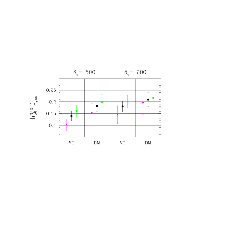
Figure 4: Bi–weight mean gas fractions at density contrasts of 500 and 200 for the VT and BM methods. Data for the full sample of 22 clusters are shown as filled circles, the low $T$ subsample of 8 clusters as triangles, and the high $T$ subsample of 14 clusters as filled squares. Error bars are $90\%$ confidence limits ($1.65\sigma$) determined from bootstrap resampling and assuming a fixed fractional error of $30\%$ on individual cluster gas fraction estimates.

Bi–weight mean gas fractions determined from a bootstrap analysis assuming fixed $30\%$ fractional errors in each measurement are listed in Table 2 and summarized in Figure 4. Data for the whole sample as well as cool and hot subsamples are provided. Uncertainties quoted in the Table are standard errors of the mean, while $90\%$ confidence errors (assuming Gaussian statistics) are plotted in the Figure.

Table 2: Bi–weight Mean Gas Fractions (%, $h_{50}^{-3/2}$)

$\hbox{$\delta_{c}$}\!=\!500$

$\hbox{$\delta_{c}$}\!=\!200$

Sample	VT	BM	VT	BM
All	$14.0\pm 1.3$	$18.3\pm 1.5$	$18.1\pm 1.4$	$21.0\pm 1.8$
$T<4{\rm\ keV}$	$10.2\pm 1.5$	$15.3\pm 2.4$	$14.5\pm 2.1$	$19.9\pm 3.2$
$T>4{\rm\ keV}$	$16.2\pm 1.5$	$20.0\pm 1.9$	$20.1\pm 1.6$	$21.6\pm 2.2$

The trend of rising gas fraction with increasing radius (lower $\delta_{c}$) is apparent with both mass estimation methods, and reflects the more extended nature of the gas density compared to the assumed or inferred dark matter profiles. Gas fraction values are consistently higher in the BM approach, due to the smaller, inferred total masses noted above. As a result, significantly different sample means can be quoted depending on the mass method and extent of radial coverage of the dataset. Compare, for example, $\hbox{${\bar{f}}_{gas}$}\!=\!0.140\pm 0.013$ for the VT at $\hbox{$\delta_{c}$}\!=\!500$ with $\hbox{${\bar{f}}_{gas}$}\!=\!0.210\pm 0.018$ for the BM at $\hbox{$\delta_{c}$}\!=\!200$.

The range becomes wider when one considers subsets of the data defined by temperature. All the panels in Figure (4) display a trend of decreasing gas fraction at lower $T$, but only the VT method at $\hbox{$\delta_{c}$}\!=\!500$ is deemed statistically significantly ($2.8\sigma$) under our $30\%$ error hypothesis. Due to the robustness of the bi–weight mean estimator, this conclusion is valid with or without the inclusion of the principal outlier A1060. It is perhaps also worth noting that the discrepancy between A1060 and the mean of the cool subsample is smaller under the VT approach.

The value of $16.2\pm 1.5\%$ for the hot subsample in the VT case is consistent with the $95\%$ confidence region $\bar{f}_{gas}(\hbox{$r_{500}$})\!=\!17.0\pm 1.7\%$ ($\hbox{$\,h_{50}$}\!=\!1$) determined by Evrard (1997) from the combined samples of White & Fabian (1995) and David, Jones & Forman (1995). Only 3 of the 26 clusters in the combined study have $T<4{\rm\ keV}$ (and these have fairly uncertain gas fractions which make negligible contribution to the sample mean), so comparison with our high–$T$ subsample is reasonable. The agreement between these two studies is not entirely trivial. Although there is nearly $50\%$ overlap with our subsample — 6 of our 14 are in common with White & Fabian — we employ here different temperature estimates in many cases (though all are consistent within the quoted errors) and we normalize the gas mass differently.

A less obvious trend in the data is the larger variance in gas fractions in the BM case compared to the VT. This is more apparent in the $T$–dependent subsamples, since the trend of mean gas fraction with temperature mimics variance in the full VT sample. The lower scatter in the VT method confirms theoretical predictions that the $\beta$ parameter acts as an extra source of noise in the BM mass estimates (EMN). An increase in scatter is also seen at larger radii/lower densities, consistent with the numerical model predictions and interpreted simply as reflecting the longer relaxation timescales in the outer regions of clusters.

4.4 Implications

There is strong evidence from the slope of the $L_{X}$–$T$ relation and from the behavior of the image fall-off parameter $\beta$ that cluster structure varies systematically with temperature. Whether the virial gas fraction varies with cluster temperature is a question whose answer is both model and scale dependent. The model dependency we highlight is the choice of total mass estimation method, while the chosen density contrast sets the scale. For example, the $\beta$–model applied at $\delta_{c}\!=\!200$ produces similar mean values in high and low temperature subsamples — $0.216\pm 0.022$ and $0.199\pm 0.032$, respectively — whereas the virial theorem at $\hbox{$\delta_{c}$}\!=\!500$ yields significantly different values in these subsamples — $0.162\pm 0.015$ against $0.102\pm 0.015$, respectively (see Table 2 and Figure 4, all values scale as $\hbox{$\,h_{50}$}^{-3/2}$).

That the implications of the observed luminosity–temperature relation are model dependent can be seen by considering the behavior of terms with temperature dependence contained in the defining relation, equation (12). The structure factor $\hat{Q}(T)$ appears to increase with temperature, but this effect is not solely responsible for the steepening of the $L_{X}$–$T$ relation. The dependence with $T$ of the other factors depends on the total mass estimation method. In the VT approach, while $\hbox{$M_{\delta_{c}}$}(T)$ scales classically as $T^{3/2}$, $f_{gas}(T)$ increases with $T$. In the BM case, while $f_{gas}$ is found to be nearly constant, the slope of the $\hbox{$M_{\delta_{c}}$}(T)-kT$ relation is steeper than $3/2$, due to the extra $\beta$ factor and its increase with $T$ (equation (19)). Both cases result in a steepening of the $f_{gas}^{2}(T)\ \hbox{$M_{\delta_{c}}$}(T)$ term to a slope greater than the canonical $3/2$. The temperature dependence of this term contributes about equally with $\hat{Q}(T)$ to the steepening of the $L_{X}$–$T$ relation.

Allan & Fabian (1998) take a different approach in analysis of a cluster dataset combining ASCA spectroscopy with ROSAT imaging. They fit ASCA data to a multi-component spectral model which includes emission from a central cooling flow (Johnstone et al. 1992), absorption from galactic hydrogen, intrinsic hydrogen absorption, and a superimposed background plasma at temperature $T$. Compared to simpler fits without cooling flow and intrinsic absorption, the best fit temperatures in their complex fits are higher, and the best fit slope of the $L_{X}$–$T$ relation is shallower, $2.33\pm 0.43$. Allen & Fabian emphasize that this slope is consistent with the straightforward theoretical expectation of $2$; however, note that the range of slopes allowed in our fit does overlap the error range quoted above (derived from a change $\delta\chi^{2}=2.71$ in their $\chi^{2}$ analysis).

The approximate nature of our error analysis limits the conclusions which can be drawn regarding gas fraction variations. A definitive analysis awaits uniform treatment of a large, homogeneous dataset. There is some supporting evidence for deficient gas fractions in poor groups (Hickson, 1997 and references therein), but there also appears to be larger scatter at low temperatures (e.g., Ponman et al. 1996) and observational uncertainties on the ICM mass remain large in these systems. In particular the separation of the ICM emission from the X–ray emission linked to individual galaxies is ambiguous and difficult with present instruments (Mahdavi et al. 1997, Mulchey and Zabludoff 1998).

5 Concluding Discussion

The narrow scatter in the $L_{X}$–$T$ relation of weak cooling flow clusters ($\dot{M}\leq 100{\rm\ M}_{\odot}{\rm\ yr}^{-1}$) indicates that the structure of the intracluster medium in this majority sub–class is very regular. Under a conservative assumption of no correlation between virial gas fraction and internal, structural variations ($\langle\delta_{Q}\delta_{f}\rangle\!=\!0$), we place upper limits on the rms percentage variation in virial gas fraction of $15\%$ for the entire sample of 24 clusters, and $9\%$ for the homogeneous GINGA subset of 18 clusters.

These limits are conservative because the X–ray imaging data supports the point of view that gas in low $T$ clusters is more extended than that of high $T$ clusters (Figure 2). Mohr & Evrard (1997) find the same result with a non–parametric analysis of X–ray images. They also derive limits on gas fraction variations similar to those found here based on the tightness of the X–ray size–temperature (ST) relation. The agreement is non–trivial because the ST analysis is essentially local, being based on an differential isophotal area, while the $L_{X}$–$T$ relation analysis is global, based an the integrated emission of the entire cluster atmosphere. Both analyses are consistent with idea that energy input from galactic winds has led to extended gas atmospheres in low $T$ clusters (David, Forman & Jones 1990,1991; White 1991; Metzler & Evrard 1997; Cavaliere et al. 1997; Ponman et al. 1996).

In wind models, gas loss is correlated with structural extension of the gas, leading to $\langle\delta_{Q}\delta_{f}\rangle>0$. The inferred variance in gas fraction derived from equation (8) could be substantially smaller than the limits phrased above if winds have played an important evolutionary role. Numerical simulations of clusters used by Mohr & Evrard (1997) exhibit less than 5% fractional variation in their virial gas fractions, and a similar value is seen in models with galactic winds (Metzler & Evrard 1997). The expected “cosmic variance” in virial gas fractions is thus quite small.

Comparison of a number of different simulation techniques paints a similar picture. Frenk et al. (1998) find agreement at the 5% level ($1\sigma$ deviation) for the virial gas fraction of a single cluster determined by twelve independent gas dynamic methods. This indicates that systematic uncertainties in the tested numerical simulation techniques are small for the simplest case of a single phase ICM. However, it is important to note that the quoted simulations ignore galaxy formation and its attendant multi–phase, gas structure. Introducing galaxy formation via cooling and star formation is likely to increase the scatter in ICM gas fraction values, and it will be interesting to see whether viable models can do so without violating the observational limits presented here.

Evidence for trends in ${\bar{f}}_{gas}$ with cluster temperature is ambiguous. A key uncertainty lies in estimation of the total, binding mass. The $\beta$–model approach produces masses which are characteristically smaller than the virial theorem method as currently calibrated by numerical simulations. For a cluster with $\beta\!=\!0.6$, the masses inferred at $\delta_{c}\!=\!500$ differ substantially, $M_{\beta}\!=\!0.66M_{VT}$. This different behavior, coupled with the temperature dependence of $\beta$, leads to differing conclusions on whether the mean gas fraction varies with cluster temperature.

For the same reason there is some ambiguity in the origin of the steepening of the $L_{X}$–$T$ relation. The fact that the gas is more concentrated in high-kT cluster explains at least half of the effect, directly through the structure factor in the X–ray luminosity. In the $\beta$–model approach, the temperature dependence of the ICM structure can fully account for the $L_{X}$–$T$ relation slope, via the additional dependence of the total mass with $\beta$. On the other hand, in the VT approach, the gas mass fraction increases with $T$ and this effect contributes about equally to the $L_{X}$–$T$ relation slope increase. Both effects, lower gas fraction and inflated gas distribution in low T systems, are expected in models incorporating the effects of galactic winds.

Independent methods for estimating virial masses are crucial, and weak gravitational lensing provides an important approach. Allen (1997) provides evidence that weak lensing and $\beta$–model mass estimates are consistent, but the present errors at radii between $r_{500}$ or $r_{200}$ are too large to discriminate between the BM and VT approaches. We suggest that weak lensing analysis of a small sample of moderate redshift clusters selected to have $\beta\mathrel{\hbox to0.0pt{\lower 3.0pt\hbox{$\mathchar 536\relax$}\hss}\raise 2.0pt\hbox{$\mathchar 316\relax$}}0.6$ from X–ray imaging could settle the score, if individual measurement uncertainties could be kept below a few tens of percent at $\delta_{c}\!=\!500$.

Future X–ray missions which provide simultaneous imaging and spectroscopic capability (AXAF, XMM, Astro-E) will provide improvements over the current dataset. The ideal analysis would be one of a flux limited sample with central, cooling flow regions excised (Markevitch 1998), using a nearly homogeneous dataset of temperatures, luminosities and surface brightness maps derived from the same telescope. Such data would minimize variance caused by instrumental uncertainties and open the door to very high precision measurements of intracluster gas fractions.

Finally, small scatter in virial gas fractions lends support to arguments against an Einstein–deSitter universe based on cluster baryon fractions and primordial nucleosynthesis (White et al. 1993; Evrard 1997). The standard counterargument to this idea has been that the physics of the ICM is more complicated than is assumed in most analytic or numerical models. However, if additional physics beyond gravity, shock heating and galactic wind input is at work in cluster ICM atmospheres, then the extra processes involved must conspire to keep the scatter in the observed $L_{X}$–$T$ and ST relations small. Since $L_{X}$ and $R_{I}$ (the “size” in the ST relation) are manifestly different measures (global vs. local), it is not obvious that interesting physical mechanisms, such as a strongly multi–phase ICM (Gunn & Thomas 1996), can be added in such a way as to preserve the current agreement between observations and current models incorporating the effects of galactic winds on the ICM.

References

- [ ] Allen S.W., 1997, MNRAS, in press, astro-ph/9710217
- [ ] Allen S.W. & Fabian, A.C. 1998, MNRAS, 297, L57.
- [ ] Arnaud M., Lachieze-Rey M., Rothenflug R., Yamashita K., Hastukade I, 1991, A&A, 243, 56
- [ ] Arnaud M., Hughes J.P., Forman W., Jones C., Lachieze Rey M., Yamashita K., Hastukade I, 1992, ApJ, 390, 345
- [ ] Arnaud, M., 1994, in Cosmological Aspects of X-ray Clusters of Galaxies, W.C. Seitter ed., NATO ASI Series, vol 441 p.197
- [ ] Arnaud M., Rothenflug R., Böhringer H., Neumann D., Yamashita, K., 1997, A&A, submitted
- [ ] Bardelli S., Zucca E., Malizia A., Zamorani G., Scaramella R., Vettolani G., 1996, A&A, 305, 435
- [ ] Bautz M.W., Mushotzky R., Fabian A.C., Yamashita K., Gendreau K.C., Arnaud K.A., Crew G.B., Tawara Y., 1994, PASJ, 46, L131
- [ ] Beers T.C., Flynn K., Gebhardt K., 1990, AJ, 100, 32
- [ ] Birkinshaw M., Hughes J.P., Arnaud K.A., 1991, ApJ, 379, 466
- [ ] Birkinshaw M., Hughes J.P., 1994, ApJ, 420, 33
- [ ] Böhringer H., Briel U.G., Schwarz R.A., Voges W., Hartner G., Trümper J., 1994, Nat, 368, 828
- [ ] Briel U.G., Henry J.P., Böhringer H., 1992, A&A259, L31
- [ ] Briel U.G., Henry J.P., 1994, Nature, 372, 439
- [ ] Bryan, G.L. & Norman, M.L. 1998, ApJ, 495, 80.
- [ ] Buote D.A., Canizares C.R., 1996, ApJ, 457, 565
- [ ] Buote D.A., Tsai J.C., 1996, ApJ, 458, 27
- [ ] Cavaliere A., Fusco-Femiano R., 1976, A&A, 49, 137
- [ ] Cavaliere A., Menci N., Tozzi P., 1997, ApJ, 484, L21
- [ ] Cirimele G., Nesci R., Trevese D., 1997 , ApJ, 475, 11
- [ ] David L.P., Arnaud K.A., Forman W., Jones C., 1990, ApJ, 356, 32
- [ ] David L.P., Forman W., Jones C., 1990, ApJ, 359, 29
- [ ] David L.P., Forman W., Jones C., 1991, ApJ, 380, 39
- [ ] David L.P., Slyz A., Jones C., Forman W., Vrtilek S.D., Arnaud K.A., 1993, ApJ, 412, 479.
- [ ] David L.P., Jones C., Forman W., 1995, ApJ, 445, 578.
- [ ] Ebeling H., 1993, phD thesis, MPE
- [ ] Ebeling H., Voges W., Böhringer H., Edge A.C., Huchra J.P., Briel J.G., 1996, MNRAS, 281, 799
- [ ] Edge A.C., 1989, phD Thesis, Leicester Univ.
- [ ] Edge A.C., Stewart G.C., Fabian A.C.J, Arnaud K.A., 1990, MNRAS, 245, 559
- [ ] Edge A.C., Stewart G.C., 1991, MNRAS, 252, 414
- [ ] Elbaz D., Arnaud M., Böringer H., 1995, A&A, 293, 337
- [ ] Evrard A.E., Henry J.P., 1991, ApJ, 383, 95
- [ ] Evrard A.E., Metzler C.A., Navarro J.F., 1996, ApJ, 469, 494.
- [ ] Evrard, A.E., 1997, MNRAS, 292, 289.
- [ ] Fabian A.C., Crawford C.S., Edge A.C., Mushotzky R.F., 1994, MNRAS, 267, 779
- [ ] Frenk C.S., White S.D.M. et al. 1998, ApJ, submitted.
- [ ] Fujita Y., Koyama K., Tsuru T., Matsumoto H., 1996, PASJ, 48, 191
- [ ] Garasi C., Burns J.O. & Loken C. 1997, BAAS, 191, 5308.
- [ ] Girardi M., Fadda D., Giuricin G., Mardirossian F., Mezzeti M., Biviano A., 1996, ApJ, 457, 61
- [ ] Girardi M., Escalera E., Fadda D., Giuricin G., Mardirossian F., Mezzeti M., 1997, ApJ, 482, 41
- [ ] Gunn K.F., Thomas P.A., 1996, MNRAS, 281, 1133
- [ ] Hatsukade I., 1989, phD Thesis, ISAS RN 435
- [ ] Henry J.P., Arnaud K.A., 1991, ApJ, 372, 410
- [ ] Hickson, P., 1997, ARA&A, 35, 357
- [ ] Hughes J.P., Tanaka Y., 1992, ApJ, 398, 62
- [ ] Hughes J.P., Butchler J.A., Stewart G.C., Tanaka Y., 1993, ApJ, 404, 611
- [ ] Johnstone, R.M., Fabian, A.C., Edge, A.C. & Thomas, P.A. 1992, MNRAS, 267, 779.
- [ ] Jones C., Forman, W., 1984, ApJ, 276, 38
- [ ] Jones C., Forman, W., 1990, private communication
- [ ] Kafuku S., Yamauchi M., Hattori H., Kawai N., Matsuoka M., 1992, in Frontiers of X-ray astronomy, ed. Y. Tanaka, K. Koyama (Universal Academay Press, Tokyo), P.483
- [ ] Loewenstein M., Mushotzky R.F., 1996, ApJ, 471, L83
- [ ] Mahdavi A., Böhringer H., Geller M., Ramella M. , 1997, ApJ, 483, 68
- [ ] Matilsky T., Jone, C., Forman W., 1985, ApJ, 291, 621
- [ ] Matsuzawa H., Matsuoka M., Ikebe Y., Mihara T., Yamashita K., 1996, PASJ, 48, 565
- [ ] McHardy I.M., Stewart G.C., Edge A.C., Cooke B., Yamashita K., Hatsukade I., 1990, MNRAS, 242, 215
- [ ] Markevitch M.L., Sarazin C.L., Irwin J.A., 1996, ApJ, 472, L17
- [ ] Markevitch M., Vikhlinin A., 1997, ApJ474, 84
- [ ] Markevitch M., 1998, ApJsubmitted, astro-ph/9802059
- [ ] Metzler C.A., 1994, in Clusters of Galaxies, eds. F. Durret, A. Mazure & J. Trân Thanh Vân (Editions Frontieres, Gif–sur–Yvette), p. 251.
- [ ] Metzler C.A., Evrard A.E., 1994, ApJ, 437, 564
- [ ] Metzler C.A., Evrard A.E., 1997, ApJ, submitted, astro-ph/9710324
- [ ] Mewe R., Gronenshild E. H. B. M., van den Oord H. J., 1985, A&A, 62, 197
- [ ] Mewe R., Lemen J.R., van den Oord H. J., 1986, A&A, 65, 511
- [ ] Mitchell R.J., Ives J.C., Culhane J.L., 1977, MNRAS, 181, 25p
- [ ] Mitchell R.J., Dickens R.J., Bell Burnell S.J., Culhane J.L., 1979, MNRAS, 189, 329
- [ ] Mohr J.J., Evrard A.E., 1997, ApJ, 1997, 491, 38
- [ ] Mushotzky R.F.,Serlemitsos P.J., Smith B.W., Boldt E.A., Holt S.S., ApJ, 225, 21
- [ ] Mulchey J.S., Zabludoff A.I., 1998, ApJ, 496, 73
- [ ] Navarro J.F., Frenk C.S., White S.D.M., 1997, ApJ, 490, 493
- [ ] Neumann, D.M, Böhringer H., 1995, A&A, 301, 865
- [ ] Ponman T.J., Bourner P.D.J., Ebeling H., Böhringer H.A. 1996, MNRAS, 283, 690.
- [ ] Takano S., 1990, PhD Thesis, Tokyo Univ. and Koyama, K., 1997, private communication
- [ ] Tamara T., Day C.S., Fukazawa Y., Hatsukade I., Ikebe Y., Makishima K., Mushotzky R.F., Ohashi T., Takenaka K., Yamashita K., 1996, PASJ, 48, 671
- [ ] Tsuru,T., 1993, phD Thesis, ISAS RN 528
- [ ] Thomas P.A., Fabian A.C., Nulsen P.E.J., 1987, MNRAS, 228, 973.
- [ ] White R.E., 1991, ApJ, 367, 69
- [1] White S.D.M., Navarro J.F., Evrard A.E., Frenk C.S., 1993, Nature, 366, 429
- [ ] White D.A., Fabian A.C., 1995, MNRAS, 273, 72.
- [ ] Yamanaka M., Fukazawa Y., private communication in Fukazawa et al., 1994, PASJ, 46, L55
- [ ] Yamashita K., 1992, in Frontiers of X-ray astronomy, ed. Y. Tanaka, K. Koyama (Universal Academay Press, Tokyo), P.475
- [ ] Yamashita K., 1997, private communication