Extragalactic Foregrounds of the Cosmic Microwave Background: Prospects for the MAP Mission

Abstract

While the major contribution to the Cosmic Microwave Background (CMB) anisotropies are the sought-after primordial fluctuations produced at the surface of last scattering, other effects produce secondary fluctuations at lower redshifts. Here, we study the extragalactic foregrounds of the CMB in the context of the upcoming MAP mission. We first survey the major extragalactic foregrounds and show that discrete sources, the Sunyaev-Zel’dovich (SZ) effect, and gravitational lensing are the most dominant ones for MAP. We then show that MAP is expected to detect ($>5\sigma$) about 46 discrete sources directly with 94 GHz fluxes above 2 Jy. The most prominent SZ features on the CMB sky are rich clusters of galaxies. In particular, we show that the Coma cluster will be clearly detected and marginally resolved by MAP. We then consider a cosmological population of clusters, and show that MAP should detect ($>5\sigma$) about 10 SZ clusters directly. The mean SZ fluxes of fainter clusters can be probed by cross-correlating MAP with cluster positions extracted from existing catalogs. For instance, a MAP-XBACs cross-correlation will be sensitive to clusters with $S(94{\rm GHz})\gtrsim 200$ mJy, and will thus provide a test of their virialization state and a measurement of their gas fraction. Finally, we consider probing the hot gas on supercluster scales by cross-correlating the CMB with galaxy catalogs. Assuming that galaxies trace the gas, we show that a cross-correlation between MAP and the APM catalog should yield a marginal detection, or at least a four-fold improvement on the COBE upper limits for the rms Compton $y$-parameter.

1 Introduction

The Cosmic Microwave Background (CMB) provides a unique probe to the early universe (see White, Scott, & Silk 1994 for a review). If CMB fluctuations are consistent with inflationary models, future ground-based and satellite experiments will yield accurate measurements of most cosmological parameters (see Zaldarriaga, Spergel, & Seljak 1997; Bond, Efstathiou, & Tegmark 1997 and reference therein). These measurements rely on the detection of primordial anisotropies produced at the surface of last scattering. However, various secondary effects produce fluctuations at lower redshifts. The study of these secondary fluctuations (or extragalactic foregrounds) is important in order to isolate primordial fluctuations. In addition, secondary fluctuations are interesting in their own right since they provide a wealth of information on the local universe.

The upcoming MAP mission (Bennett et al. 1995) will produce a map of the CMB sky with unprecedented sensitivity, frequency coverage, and angular resolution. In this paper, we study the extragalactic foregrounds of the CMB in the context of MAP. After surveying the major sources of secondary anisotropies, we show that discrete sources, the Sunyaev-Zel’dovich (SZ) effect, and gravitational lensing are the dominant extragalactic foregrounds for MAP. The SZ effect is produced by the comptonization of CMB photons by the hot gas in clusters and superclusters of galaxies along the line of sight. Searches for extragalactic foregrounds have been performed in the COBE maps, but have only led to upper limits (Boughn & Jahoda 1993; Bennett et al. 1993; Banday et al. 1996; Kneissl et al. 1997). We focus on discrete and SZ foregrounds and show how they affect future CMB maps. In addition, we present statistical techniques to detect SZ fluctuations beyond the threshold of direct detection for MAP, by cross-correlating CMB maps with existing galaxy and cluster catalogs. While the present analysis was developed in the context of MAP, many of the techniques will also be useful for other experiments (esp. Planck Surveyor; Bersanelli et al. 1996).

In §2, we briefly describe the characteristics of MAP which are relevant to the present study. In §3, we review the major sources of secondary anisotropies, and quantify their relative importance for MAP. In §4, we estimate, using existing models, the number of discrete sources detectable with MAP. In §5, we turn to the contribution of the SZ Effect to CMB maps. We first survey the most prominent SZ sources in the sky (§5.1), and then consider the SZ effect by a cosmological population of clusters (§5.2), and by superclusters (§5.3). Finally, §6 summarizes our conclusions.

2 MAP Sensitivity

The MAP instrument will comprise 5 channels with frequencies between 20 and 94 GHz. A detailed description of the MAP mission can be found in Bennett et al. 1995. Foregrounds can be optimally separated using multi-frequency filtering techniques (Bersanelli et al. 1996; Tegmark & Efstathiou 1996; Bouchet et al. 1998). As we will see below, extragalactic foregrounds are, for the most part, only weakly dependent on frequency in the MAP frequency range. (Even for discrete sources, the improvement yielded by a multi-channel analysis is limited by the presence of flat-spectrum sources; see §4). As a first step and to be conservative, we thus presently only consider the W-band channel which has the highest angular resolution.

Assuming the current design with 2 years of coverage, the combined W-band detectors have a center frequency of $\nu\simeq 94$ GHz, a beam FWHM of $\theta_{\rm beam}\simeq 0.21$ deg, and an instrumental rms noise of $\Delta T_{\rm pix}\simeq 35\mu$K (thermodynamic temperature) per $\Omega_{\rm pix}=\theta_{\rm pix}^{2}=0\fdg 3\times 0\fdg 3$ pixels.

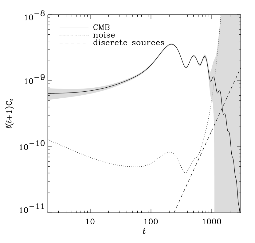
Figure 1: Power spectrum sensitivity for the 94 GHz MAP channel. The solid line corresponds to a COBE normalized standard CDM model with $\Omega_{b}=0.05$ and $h=0.5$. The shaded region and the dotted line show the rms sensitivity for the MAP 94 GHz channel with a 2 year, full sky coverage and a bandpass average of $\Delta\ell=10$. The dashed line shows the power spectrum for residual discrete sources with $S(94{\rm GHz})<S_{94}(5\sigma)\simeq 2$ Jy, as extrapolated from Toffolatti et al. (1998).

The temperature fluctuations measured by MAP are decomposed into the usual spherical harmonics basis, $\frac{\delta T}{T_{0}}(\mbox{\bf$\theta$})=\sum_{\ell,m}a_{\ell m}Y_{\ell m}(\mbox{\bf$\theta$})$, where the $a_{\ell m}$’s are the multipole moments. Here, $T_{0}\simeq 2.725$K is the mean CMB temperature (Mather et al. 1998). As a reference, the averaged multipole moments $C_{\ell}\equiv\langle|a_{\ell m}|^{2}\rangle$ for a COBE-normalized standard CDM model (with $\Omega_{b}=0.05$, and $h=0.5$) calculated with CMBFAST (Seljak & Zaldarriaga 1996) are shown in figure 1.

The rms uncertainty $\Delta C_{\ell}$ for measuring $C_{\ell}$ averaged over a bandpass of width $\Delta\ell$ is given by (eg. Knox 1995)

$$\Delta C_{\ell}=\left(\frac{2}{2\ell+1}\right)^{\frac{1}{2}}\left[C_{\ell}+\left(\frac{\Delta T_{\rm pix}}{T_{0}}\right)^{2}\Omega_{\rm pix}W_{\ell}^{-1}\right](f_{\rm sky}\Delta\ell)^{-\frac{1}{2}}$$ (1)

where $\Delta T_{\rm pix}$ is the thermodynamic noise per pixel, $\Omega_{\rm pix}$ is the pixel solid angle, and $f_{\rm sky}$ is the fraction of the sky covered (with randomly-positioned discarded pixels). Taking the beam to be gaussian with a standard deviation of $\sigma_{\rm beam}$, the window function $W_{\ell}$ is given by $W_{\ell}=e^{-\ell^{2}\sigma_{\rm beam}^{2}}$. The first and second terms correspond to cosmic variance and instrumental noise, respectively. The measurement uncertainty $\Delta C_{\ell}$ for the MAP 94 GHz channel is shown in figure 1 both as the shaded regions and as the dotted line. A 2-year coverage of the full sky and a bandpass width of $\Delta\ell=10$ was assumed.

The zero-lag temperature variance is given by

$$(\Delta T)^{2}=\sum_{\ell}\frac{2\ell+1}{4\pi}C_{\ell}W_{\ell}F_{\ell}T_{0}^{2},$$ (2)

where $W_{\ell}$ is the beam window function defined above. The factor $F_{\ell}$ is an optional filter function (see below) and should be set to 1 in the unfiltered case. For the above CDM model , the unfiltered rms CMB fluctuation smoothed with the W-band beam is $\Delta T_{\rm CMB}\simeq 92\mu$K. The smoothed rms fluctuation $\Delta T_{\rm inst}$, produced by the instrumental noise, is related to the pixel rms noise $\Delta T_{\rm pix}$ by $\Delta T_{\rm inst}=(4\pi)^{-\frac{1}{2}}\theta_{\rm pix}\sigma_{\rm beam}^{-1}\Delta T_{\rm pix}$. For the MAP 94 GHz channel, the smoothed (unfiltered) instrumental noise is thus $\Delta T_{\rm inst}\simeq 33\mu$K.

For the detection of spatially compact sources, the CMB fluctuations can be reduced by filtering out low spatial frequencies. Specifically, we choose a gaussian filter function of the form $F_{\ell}=1-e^{-\ell(\ell+1)\sigma^{2}_{\rm filter}}$ (see Tegmark & Oliveira-Costa 1997, for a more sophisticated treatment). For a filter with FWHM $\theta_{\rm filter}\equiv\sigma_{\rm filter}\sqrt{8\ln 2}=1^{\circ}$, the resulting rms fluctuation is $\Delta T_{\rm CMB,filtered}\simeq 65\mu$K, for the same model. Upon filtering, the instrumental noise rms fluctuation becomes $\Delta T_{\rm inst,filtered}\simeq 32\mu$K and is thus hardly affected. The resulting total rms “noise” produced by the combination of CMB and instrumental noise is then

$$\Delta T_{\rm noise}\simeq 73~{}\mu{\rm K}.$$ (3)

We will use this figure when considering the detection of foreground sources.

For future reference, we compute the sensitivity of MAP for point source detections. For a 94 GHz map smoothed with a gaussian beam, the peak temperature offset produced by an unresolved source with flux $S(94{\rm GHz})\equiv S_{94}$ is

$$\Delta T_{94}\simeq 301\left(\frac{0.21{\rm deg}}{\theta_{\rm beam}}\right)^{2}\left(\frac{S_{94}}{1{\rm Jy}}\right)\mu{\rm K}.$$ (4)

The corresponding $1\sigma$ threshold for the detection of point sources is thus

$$S_{94}(1\sigma)\simeq 250\left(\frac{\Delta T_{\rm noise}}{75\mu{\rm K}}\right){\rm mJy},$$ (5)

where the central value for $\Delta T_{\rm noise}$ was chosen to be close to that of equation (3).

3 Overview of Extragalactic Foregrounds

In this section, we survey the major extragalactic foregrounds and secondary anisotropies of the CMB by relying on existing literature. To assess their relative importance, we follow Tegmark & Efstathiou (1996) and consider the quantity $\Delta T_{\ell}\equiv\left[\ell(2\ell+1)C_{\ell}/4\pi\right]^{\frac{1}{2}}T_{0}$, which gives the rms temperature fluctuations per $\ln\ell$ interval centered at $\ell$. Another useful quantity that they considered is the value of $\ell=\ell_{eq}$ for which foreground fluctuations are equal to the CMB fluctuations, i.e. for which $C_{\ell}^{\rm foreground}\simeq C_{\ell}^{\rm CMB}$. Note that, since the foregrounds do not necessarily have a thermal spectrum, $\Delta T_{\ell}$ and $\ell_{eq}$ generally depend on frequency.

We present our results both in table 1 and in figure 2. In the table, we list $\Delta T_{\ell}$ and $\ell_{eq}$ for each of the major extragalactic foregrounds at $\nu=94$ GHz and $\ell=450$, which corresponds to a FWHM angular scale of about $\theta\sim.3$ deg. These values were chosen to be relevant to the MAP W-band ($\nu\simeq 94$ GHz and $\theta_{\rm beam}\simeq 0\fdg 21$, see §2). We also indicate whether each foreground component has a thermal spectrum.

Figure 2 summarizes the importance of each of the extragalactic foregrounds in the multipole-frequency plane. It should be compared to the analogous plot for galactic foregrounds (and discrete sources) shown in Tegmark & Efstathiou (1996; see also Tegmark 1997 for an updated version). These figures show regions on the $\ell$-$\nu$ plane in which the foreground fluctuations exceed the CMB fluctuations, i.e. in which $C_{\ell}^{\rm foreground}>C_{\ell}^{\rm CMB}$. As a reference for $C_{\ell}^{\rm CMB}$, we have used the CDM model shown in figure 1. Also shown in figure 2 is the region in which MAP is sensitive, i.e. in which $\Delta C_{\ell}^{\rm noise}<C_{\ell}^{\rm CMB}$, where $\Delta C_{\ell}^{\rm noise}$ is the rms uncertainty for MAP (see Eq. [1]). A similar region is shown for the current design parameters of Planck surveyor (Bersanelli et al. 1996) . Note that this figure is only intended to illustrate the domains of importance of the different foregrounds qualitatively.

In the following, we briefly describe each extragalactic foreground and comment on its respective entries in table 1 and figure 2.

3.1 Discrete Sources

Discrete sources produce positive, point-like, non-thermal, and possibly time-variable fluctuations. While not much is known about discrete source counts around $\nu\sim 100$ GHz, several models have been constructed by interpolating between radio and IR observations (Toffolatti et al. 1998; Gawiser & Smoot 1997; Gawiser et al. 1998; Sokasian et al. 1998). Here, we adopt the model of Toffolatti et al. and consider the two flux limits $S<1$ and 0.1 Jy for the source removal in table 1. The sparsely dotted region figure 2 shows the discrete source region for $S<1$ Jy. In the context of CMB experiments, the Poisson shot noise dominates over clustering for discrete sources (see Toffolatti et al. ). As a result, the discrete source power spectrum, $C_{\ell}^{\rm discrete}$, is essentially independent of $\ell$. Discrete sources are discussed in more details in §4.

3.2 Thermal Sunyaev-Zel’dovich Effect

The hot gas in clusters and superclusters of galaxies affect the spectrum of the CMB through inverse Compton scattering. This effect, known as the Sunyaev-Zel’dovich (SZ) effect (for reviews see Sunyaev & Zel’dovich 1980; Rephaeli 1995), results from both the thermal and bulk motion of the gas. We first consider the thermal SZ effect, which typically has a larger amplitude and has a non-thermal spectrum (see the §3.3 below for a discussion of the kinetic SZ effect). The CMB fluctuations produced by the thermal SZ effect have been studied using the Press-Schechter formalism (see Bartlett 1997 for a review), and on large scales using numerical simulations (Cen & Ostriker 1992; Scaramella, Cen, & Ostriker 1993) and semi-analytical methods (Persi et al. 1995). For our purposes, we consider the SZ power spectrum, $C_{\ell}^{\rm SZ}$, calculated by Persi et al. (see their figure 5). In table 1, we consider their calculation both with and without bright cluster removal. In figure 2, only the spectrum without cluster removal is shown. A more complete discussion of the SZ effect is given in §5.

3.3 Ostriker-Vishniac Effect

In addition to the thermal SZ effect described above, the hot intergalactic medium can produce thermal CMB fluctuations as a result of its bulk motion. While this effect essentially cancels to first order, the second order term in perturbation theory, the Ostriker-Vishniac (OV) effect (Ostriker & Vishniac 1986; Vishniac 1987), can be significant on small angular scales. The power spectrum of the OV effect depends on the ionization history of the universe, and has been calculated by Hu & White (1996), and Jaffe & Kamionkowski (1998; see also Persi et al. 1995). We use the results of Hu & White (see their figure 5) who assumed that the universe was fully reionized beyond a redshift $z_{r}$. In table 1, we consider the two values $z_{r}=10$ and 50, while in figure 2, we only plot the region corresponding to $z_{r}=50$. For consistency, we still use the standard CDM power spectrum as a reference, even though the primordial power spectrum would be damped in the event of early reionization. (Using the damped primordial spectrum makes, at any rate, only small corrections to both table 1 and figure 2.)

3.4 Integrated Sachs-Wolfe Effect

The Integrated Sachs-Wolfe Effect (ISW) describes thermal CMB fluctuations produced by time variations of the gravitational potential along the photon path (Sachs & Wolfe 1967). Linear density perturbations produce non-zero ISW fluctuations in $\Omega_{m}\neq 1$ universe only. Non-linear perturbations produce fluctuations for any geometry, an effect often called the Rees-Sciama effect (Rees & Sciama 1968). Tuluie & Laguna (1995) have shown that anisotropies due to intrinsic changes in the gravitational potentials of the inhomogeneities and anisotropies generated by the bulk motion of the structures across the sky generate CMB anisotropies in the range of $10^{-7}\lesssim\frac{\Delta T}{T}\lesssim 10^{-6}$ on scales of about $1^{\circ}$ (see also Tuluie et al. 1996). The power spectrum of the ISW effect in a CDM universe was computed by Seljak (1996a; see also references therein). In table 1, we consider values of the density parameter, namely $\Omega h=0.25$ and 0.5. In figure 2, only the $\Omega h=0.25$ case is shown. As above, the standard CDM ($\Omega=1$, $h=0.5$) spectrum is still used as a reference.

3.5 Gravitational Lensing

Gravitational lensing is produced by spatial perturbations in the gravitational potential along the line of sight (see Schneider, Ehlers, & Falco 1992; Narayan & Bartelmann 1996). This effect does not directly generate CMB fluctuations, but modifies existing background fluctuations. The effect of lensing on the CMB power spectrum was calculated by Seljak (1996b) and Metcalf & Silk (1997). Recently, Zaldarriaga & Seljak (1998) included the lensing effect in their CMB spectrum code (CMBFAST; Seljak & Zaldarriaga 1996). We use this code to compute the absolute lensing correction $|\Delta C_{\ell}^{\rm lens}|$ to the standard CDM spectrum of figure 1, including nonlinear evolution. The results are shown in table 1 and figure 2.

3.6 Other Extragalactic Foregrounds

In addition to the effects discussed above, other extragalactic foregrounds can cause secondary anisotropies. For instance, patchy reionization produced by the first generation of stars or quasars can cause second order CMB fluctuations through the doppler effect (Aghanim et al. 1996a,b; Gruzinov & Hu 1998; Knox, Scoccimaro, & Dodelson 1998; Peebles & Juzkiewicz 1998). Calculations of the spectrum of this effect are highly uncertain, but show that the resulting CMB fluctuations could be of the order of 1 $\mu$K on 10 arcminute scales, for extreme patchiness. More likely patchiness parameters make the effect negligible on these scales, but potentially important on arcminute scales. Another potential extragalactic foreground is that produced by the kinetic SZ effect from Ly_α absorption systems, as was recently proposed by Loeb (1996). The resulting CMB fluctuations are of the order of a few $\mu$K on arcminute scales, and about one order of magnitude lower on 10 arcminute scales. Because of the uncertainties in the models for these two foregrounds and because they are small on 10 arcminute scales, we do not include them in table 1 and figure 2.

3.7 Comparison

An inspection of table 1 shows that, for MAP, the power spectra of the largest extragalactic foregrounds considered are a factor of 5 below the primordial CDM spectrum. As can be seen in figure 2, the dominant foregrounds for MAP are discrete sources, the thermal SZ effect and gravitational lensing. Note that for Planck surveyor, these three effects produce fluctuations which are close to the sensitivity of the instrument. The spectra of the OV and ISW effects will produce fluctuations of the order of $1\mu$K for MAP, and are thus less important. The effect of gravitational lensing is now incorporated in CMB codes such as CMBFAST, and can thus be taken into account in the estimation of cosmological parameters. The other two dominant extragalactic contributions, discrete sources and the thermal SZ effect, must also be accounted for, but are more difficult to model. We focus on these two foregrounds in the following sections. Note that, on large angular scales, extragalactic foregrounds produce relatively small fluctuations, and are thus not detectable in the COBE maps (Boughn & Jahoda 1993; Bennett et al. 1993; Banday et al. 1996; Kneissl et al. 1997)

4 Discrete Sources

In this section, we use the existing literature to estimate the discrete source contribution to the 94 GHz MAP channel. Since discrete sources generally have spectra that differ from that of the CMB, this single-channel analysis should be viewed as being conservative. Note, however, that for the sizable fraction of radio sources which have a flat spectrum (see Sokasian et al. 1998), a multi-channel analysis will not dramatically improve the source subtraction. Indeed, the Rayleigh-Jeans (RJ) temperature fluctuations produced by such sources (with fluxes $S_{\nu}\propto\nu^{0}$) depend on frequency as $\Delta T\propto S_{\nu}\theta_{\rm beam}^{-2}\nu^{-2}\propto\nu^{0}$ since $\theta_{\rm beam}\propto\nu^{-1}$ approximately for MAP, and are thus indistinguishable from CMB fluctuations. Source subtraction can also be improved by searching the time-ordered data for time-variability, which is common for radio sources. It can also be improved by cross-correlating the CMB maps with existing source catalogs (eg. that by Sokasian et al. 1998; for searches in the COBE maps see Bennett et al. 1993; Banday et al. 1996; see also §22 below for an application of this technique to SZ clusters).

4.1 Source Counts

Toffolatti et al. (1998) have computed the expected discrete source counts based on radio and IR surveys. An extrapolation of the Toffolatti et al. counts to 94 GHz yields an integrated source density of

$$n_{\rm disc}(>5\sigma)\simeq 2.2\times 10^{-3}{\rm~{}sources~{}deg}^{-2},$$ (6)

where the flux threshold is the $5\sigma$ detection threshold for the MAP 94 GHz channel, $S_{94}(5\sigma)\approx 2$ Jy (see Eq. [5]). The corresponding number of sources directly detectable by MAP is

$$N_{\rm disc}(>5\sigma)\simeq 46\left(\frac{f_{\rm sky}}{0.5}\right){\rm~{}sources},$$ (7)

where $f_{\rm sky}$ is the fractional sky coverage resulting from the galactic cut. As a comparison, the expected number of random $>5\sigma$ fluctuations in $0\fdg 3\times 0\fdg 3$ pixels is $N_{\rm random}(>5\sigma)\simeq 0.27f_{\rm sky}$.

The contribution of discrete sources to the microwave sky has also been investigated by Gawiser & Smoot (1997), Gawiser et al. (1998), and Sokasian et al. (1998). In particular, Sokasian et al. have used a catalog of 2200 bright extragalactic sources, over 700 of which have been observed at 90 GHz. They predict $N_{\rm disc}(>5\sigma)\simeq 25$ for the 94 GHz MAP channel with $f_{\rm sky}=0.5$. This is about a factor of 2 below the above prediction from Toffolatti et al. This discrepancy is acceptable given the uncertainties involved in the source surveys and models.

4.2 Residual Variance

Unless external catalogs are used, sources with fluxes less than $S_{94}(5\sigma)$ will contaminate the CMB maps. Ignoring source clustering (see Toffolatti et al. 1998), the CMB fluctuations from discrete sources are dominated by Poisson shot noise which is independent of $\ell$. (For the 94 GHz channel, the clustering variance is about 4 times lower than the Poisson variance, and is ignored in this analysis; see Toffolatti et al. ). A mild extrapolation of the source power spectrum of Toffolatti et al. yields

$$C_{\ell}^{\rm disc}(94{\rm GHz},<5\sigma)\simeq 1.71\times 10^{-16},$$ (8)

for all $\ell$. Euclidean counts ($N(>S)\propto S^{-3/2}$) were assumed to extrapolate the 94 GHz flux limit to $S_{94}(5\sigma)$. The resulting temperature rms fluctuations for the MAP 94 GHz channel is (See Eq. [2] with $F_{\ell}\equiv 1$)

$$\Delta T_{\rm disc}\simeq 6.5\mu{\rm K}.$$ (9)

Note that this figure includes contribution from all the multipoles, while the related entries in table 1 refer only to a $\Delta\ln\ell=1$ interval around $\ell=450$. The discrete source power spectrum is shown as the dashed line in figure 1. The discrete source fluctuations are well below the CMB fluctuations for all relevant $\ell$’s. However, they are comparable to the 94 GHz channel noise for $\ell\sim 700$. Discrete sources must therefore be carefully accounted for when estimating cosmological parameters with MAP. This can be achieved by calibrating the discrete source power spectrum (Eq. [8]) by counting the number of detectable sources in the map (Eq. [7]).

4.3 Residual Skewness

The residual discrete sources will not only contribute to the CMB variance but also to its skewness. To estimate the resulting skewness, let us consider the discrete source statistics in $N_{\rm pix}$ pixels of solid angle $\Omega_{\rm pix}$. The mean number of sources brighter than the flux detection threshold $S_{d}$ in such a pixel is $N(>S_{d})=\Omega_{\rm pix}\int_{S_{d}}^{\infty}dS\frac{dn}{dS}$, where $\frac{dn}{dS}$ is the differential source count per unit solid angle. The statistics of the unresolved background due to all sources with fluxes below $S_{d}$ can be quantified using the moments of the differential counts defined as $Q_{\alpha}\equiv\Omega_{\rm pix}\int_{0}^{S_{d}}dSS^{\alpha}\frac{dn}{dS}$. The mean unresolved intensity in a pixel is then $<I>=Q_{1}$. The intensity variance and skewness are $\sigma^{2}_{\rm disc}\equiv\langle\left(I-\langle I\rangle\right)^{2}\rangle=Q_{2}$ and $\eta_{\rm disc}\equiv\langle\left(I-\langle I\rangle\right)^{3}\rangle=Q_{3}$, respectively. To derive the last expressions, we assumed that the source counts obey Poisson statistics, thereby ignoring source clustering. For the MAP detection threshold ($S_{d}=S_{94}(5\sigma)\simeq 2$ Jy), the former integrals are dominated by counts close to $S_{d}$ which are nearly Euclidean. We therefore approximate $\frac{dn}{dS}\propto S^{-5/2}$. In this case, it is easy to show that $\sigma_{\rm disc}^{2}=3N(>S_{d})S_{d}^{2}$ and $\eta_{\rm disc}=N(>S_{d})S_{d}^{3}=\frac{1}{3}\sigma_{\rm disc}^{2}S_{d}$.

Let us then determine whether discrete sources can produce a detectable skewness. For this purpose, let us assume that the intrinsic CMB fluctuations (along with instrumental noise) are gaussian distributed. In this case, CMB fluctuations have vanishing skewness, i.e. $\eta_{\rm CMB}=0$. The $1\sigma$ uncertainty in measuring this zero skewness is $\sigma[\eta_{\rm CMB}]=\sqrt{\frac{6}{N_{pix}}}\sigma_{\rm CMB}^{3}$, where $\sigma^{2}_{\rm CMB}$ is the variance of the CMB fluctuations. As a result, the signal-to-noise ratio for detecting the discrete source skewness in the maps is SNR${}_{\eta}\equiv\eta_{\rm disc}\sigma^{-1}[\eta_{\rm CMB}]$. Combining this with the above Euclidean approximations, we get SNR${}_{\eta}\simeq(6N_{\rm pix})^{-\frac{1}{2}}{\rm SNR}_{d}^{3}N_{\rm disc}(>S_{d})$, where SNR${}_{d}\equiv S_{d}\sigma_{\rm CMB}^{-1}$ is the signal-to-noise ratio for the detection, and $N_{\rm disc}(>S_{d})=N_{\rm pix}N(>S_{d})$ is the total number of detected sources in the map. The number of pixels $N_{\rm pix}$ is related to the fraction of the sky covered $f_{\rm sky}$ by $N_{\rm pix}=4\pi f_{\rm sky}\Omega_{\rm pix}^{-1}$. For the MAP 94 GHz channel with $0\fdg 3\times 0\fdg 3$ pixels, we get

$${\rm SNR}_{\eta}\simeq 4.9\left(\frac{f_{\rm sky}}{0.5}\right)^{\frac{1}{2}}\left(\frac{{\rm SNR}_{d}}{5}\right)^{3}\left(\frac{n(>S_{d})}{2.2\times 10^{-3}{\rm deg}^{-2}}\right).$$ (10)

We therefore expect the skewness from discrete sources to be detectable at the $\sim 5\sigma$ level. Care must be taken that this skewness is not mistaken for the intrinsic CMB skewness.

5 Thermal Sunyaev-Zel’dovich Effect

As we discussed in §3.2, the thermal SZ effect describes the inverse Compton scattering of CMB photons with the hot gas in clusters and superclusters of galaxies. The resulting change in the (thermodynamic) CMB temperature observed at frequency $\nu$ is given by

$$\frac{\Delta T_{SZ}}{T_{0}}=yj(x),$$ (11)

where $T_{0}$ is the unperturbed CMB temperature, $y$ is the comptonization parameter, $x$ is a dimensionless parameter defined as $x\equiv\frac{h\nu}{kT_{0}}$, and $j(x)$ is a spectral function. The Compton parameter is given by

$$y=\int dl\frac{kT_{e}}{m_{e}c^{2}}\sigma_{T}n_{e},$$ (12)

where $T_{e}$ is the electron temperature, $n_{e}$ is the electron density, $\sigma_{T}$ is the Thompson cross-section, and the integral is over the line-of-sight distance. In the nonrelativistic regime ($kT_{e}\ll m_{e}c^{2}$), the spectral function is

$$j(x)=\frac{x\left(e^{x}+1\right)}{e^{x}-1}-4$$ (13)

which is zero at $x_{0}\simeq 3.83$, corresponding to $\nu_{0}\simeq 217$ GHz for $T_{0}=2.725$ K. The SZ temperature shift $\Delta T_{SZ}$ is negative (positive) for observation frequencies $\nu$ below (above) $\nu_{0}$. In the RJ limit ($x\ll 1$), the spectral function becomes $j(x\ll 1)\simeq-2$. For the MAP W-channel $(\nu\simeq 94$ GHz), $x=x_{94}\simeq 1.65$ and $j(x_{94})\equiv j_{94}\simeq-1.56$.

In the following, we study the impact of the SZ effect on MAP. In §5.1, we estimate the SZ decrement for prominent clusters of galaxies. In §5.2, we consider a cosmological population of cluster via both the Press-Schechter formalism and existing X-ray cluster catalogs. Finally, we study the SZ effect from hot gas on supercluster scales in §5.3.

5.1 Prominent SZ sources

We begin by surveying the most prominent SZ sources in the sky and establishing their relevance for MAP. Note that a search for the SZ effect of nearby clusters of galaxies in the COBE-DMR maps has only led to upper limits (Kogut et al. 1994).

For this purpose, we will make use of the isothermal $\beta$-model which is commonly used to fit cluster profiles. In this model, the 3-dimensional electron density $n_{e}(r)$ is taken to be spherical with a profile given by

$$n_{e}(r)=n_{0}\left[1+\left(\frac{r}{r_{c}}\right)^{2}\right]^{-\frac{3}{2}\beta},$$ (14)

where $n_{0}$ is the central electron density, $r_{c}$ is the core radius, and $\beta$ is the slope parameter. For an isothermal cluster with temperature $T_{e}$, the resulting angular SZ profile (Eq. [11]) is

$$\Delta T_{SZ}(\theta)=\Delta T_{SZ}(0)\left[1+\left(\frac{\theta}{\theta_{c}}\right)^{2}\right]^{-\frac{3}{2}\beta+\frac{1}{2}},$$ (15)

where $\theta_{c}\equiv r_{c}/D_{A}$ is the projected core radius and $D_{A}$ is the angular diameter radius. The central SZ decrement $\Delta T_{SZ}(0)$ (Eqs. [11] & [12]) is related to the central electron density $n_{0}$ as

$$\Delta T_{SZ}(0)\simeq-38.8\mu\mbox{\rm K}\left(\frac{n_{0}}{10^{-3}\mbox{\rm cm}^{-3}}\right)\left(\frac{kT_{e}}{1\mbox{\rm keV}}\right)\left(\frac{r_{c}}{1\mbox{\rm Mpc}}\right)\left(\frac{j(x)}{-2}\right)\frac{\Gamma(3\beta/2-1/2)}{\Gamma(3\beta/2)},$$ (16)

where $j(x)$ is the spectral function defined in Eq. (13), and $\Gamma$ is the gamma function. In practice, the central electron density can be determined from observations of the X-ray intensity profile which scales as $i_{x}(\theta)\propto n_{0}^{2}\left[1+\left(\frac{\theta}{\theta_{c}}\right)^{2}\right]^{-3\beta+\frac{1}{2}}$.

• The Local Group: The hot gas in the Local Group (LG) surrounds the Milky Way and can thus, in principle, contribute to the CMB quadrupole (Suto et al. 1996). In general, one expects the CMB and LG quadrupoles to contribute to the total quadrupole $Q_{\rm tot}$ as $Q_{\rm tot}^{2}=Q_{\rm CMB}^{2}+Q_{LG}^{2}$, where $Q^{2}\equiv 5C_{2}T_{0}^{2}/4\pi$. However, Pildis & McGaugh (1996) showed that the LG quadrupole is of the order of $Q_{\rm LG}\sim 0.1\mu$K for $\beta$-models of the LG which are consistent with observations of poor, spiral-dominated groups. This is well below the quadrupole measured by COBE, $Q_{\rm COBE}=10.0^{+3.8}_{-2.8}\mu$K ($1\sigma$; Bennett et al. 1996), and the cosmic variance uncertainty, $\Delta Q\simeq 3.2\mu$K (see Eq. [1]). Thus, unless the LG is a very peculiar group, its SZ effect on the CMB is negligible.

• Virgo: Virgo is at a distance of about 18 Mpc and is thus the nearest cluster. X-ray observations of Virgo (Böhringer et al. 1994; Nulsen & Böhringer 1995) show highly irregular emission with a temperature of $kT_{e}\simeq 2.4$ keV. A fit to the X-ray profile derived from the ROSAT All-Sky Survey (Böhringer 1998) yields the following $\beta$-model parameters: $\theta_{c}\simeq 2\farcm 65$, $\beta\simeq 0.47$, and $n_{0}\simeq 0.029$ cm^-3. The resulting central SZ temperature at $\nu=94$ GHz is $\Delta T_{\rm SZ}(0)\simeq-113\mu$K (Eq. [16]). The SZ profile derived for these parameters (Eq. [15]) is shown in figure 3. Also shown are the $1\sigma$ detection threshold (Eq. [3]) and $1\sigma$ beam radius for the 94 GHz MAP channel. Virgo is thus rather extended, but has a central SZ decrement which is only $1.5\sigma$ above the MAP detection threshold.

• Coma: Coma is at $z\simeq 0.02$ and is the nearest massive cluster. Fits of a $\beta$-model to X-ray observations (Hughes, Gorenstein, & Fabricant 1988; Briel, Henry, & Böhringer 1992) yields: $kT_{x}\simeq 9.1$ keV, $\theta_{c}\simeq 10\farcm 5$, and $\beta\simeq 0.75$. The SZ effect for Coma was detected by Herbig et al. (1995) who found a RJ central decrement of $\Delta T_{\rm SZ}(0)=-505\pm 92$ $\mu$K. The resulting 94 GHz SZ profile (Eq. [15]) is shown in figure 3. Coma will be clearly detected ($>5\sigma$ in the central pixel) and marginally resolved by MAP.

• Unresolved Bright Clusters: In addition, about 10 clusters will be detectable by MAP at the $>5\sigma$ level. Table 2 shows the 12 clusters which are expected to yield the largest SZ flux in the XBACs catalog (see §5.2.2). A study of the SZ effect produced by a cosmological population of clusters is the object of the next section.

5.2 Cosmological Cluster Population

In addition to the above prominent clusters, the population of clusters distributed throughout the universe will produce SZ fluctuations in the CMB. We estimate the SZ cluster counts for MAP by considering both predictions from the Press-Schechter formalism and existing X-ray cluster catalogs.

5.2.1 Press-Schechter Predictions

The Press-Schechter formalism (PS; Press & Schechter 1974) can be used to predict the SZ cluster counts in a given cosmology (De Luca, Désert, & Puget 1995; Barbosa et al. 1996; Colafrancesco et al. 1997; see also Aghanim et al. 1997 and the review by Bartlett 1997). For our purposes, we use the PS predictions of De Luca et al. (1995) who considered a CDM model with $n=1$, $b=1.7$, $\Omega_{0}=1$, and $h=0.5$. Their normalization was chosen to match the observed X-ray and optical cluster counts. For fluxes above $S_{94}\simeq 2$ mJy, the integrated counts are nearly Euclidean and given by

$$n(>S_{94})\simeq 0.043\left(\frac{S_{94}}{100{\rm mJy}}\right)^{-\frac{3}{2}}{\rm deg}^{-2},$$ (17)

where fluxes have been converted to $S_{94}\equiv S(94{\rm GHz})$. The differential $dn/dS$ and integrated $n(>S)$ counts are shown in Figure 4.

5.2.2 Empirical predictions

Cluster counts can also be empirically predicted by considering existing cluster catalogs. For this purpose, we utilize the XBACs catalog (Ebeling et al. 1996) which consists of a nearly complete, X-ray flux limited, sample of Abell-type clusters detected in the ROSAT All Sky Survey. The survey consists of 242 optically selected clusters with $z<0.2$, $|b|>20^{\circ}$, and $S_{x}(0.1-2.4{\rm keV})<5\times 10^{-12}$ erg s^-1 cm^-2. When available, the future BCS cluster catalog (see Ebeling et al. 1997) will be X-ray selected and will thus be even more suited to the present study.

The SZ fluxes of clusters can be estimated from their X-ray properties using the virial theorem. Indeed, the X-ray temperature of a virialized cluster is related to its mass by $T_{e}\propto M^{\frac{2}{3}}$. Such a relation was verified to hold well in the numerical simulations of Evrard, Metzler, & Navarro (1996) who found the proportionality constant to be

$$kT_{e}\simeq 1.27\left(\frac{M}{10^{14}M_{\odot}}\right)^{\frac{2}{3}}{\rm keV}.$$ (18)

Here, $M$ is the mass within the virialized region, which is approximated to the region corresponding to a density contrast of $\delta=500$. The dispersion between the above mass estimates and that from numerical simulations was found by Evrard et al. to have a standard deviation of less than 15%.

The total flux $S_{\nu}$ of a cluster observed at frequency $\nu$ is related to the angular integral of the thermodynamic temperature shift $\Delta T_{\nu}$ by

$$S_{\nu}=\frac{2k^{3}T_{0}^{2}}{h^{2}c^{2}}q(x)\int d\Omega~{}\Delta T_{\nu}(\mbox{\bf$\theta$}),$$ (19)

where $q(x)\equiv x^{4}/(2\sinh\frac{x}{2})^{2}$ is a spectral function, and $x\equiv h\nu/kT_{0}$ as before. For the MAP W-channel ($\nu=94$ GHz, $x=x_{94}\simeq 1.65$), $q(x_{94})\equiv q_{94}\simeq 2.18$. By inserting equations (11) and (12) into the above expression, it is easy to see that the total SZ flux of a virialized cluster scales as $S_{\rm SZ}\propto f_{\rm gas}MT_{e}\propto f_{\rm gas}T_{e}^{\frac{5}{2}}$. where $f_{\rm gas}\equiv M_{\rm gas}/M$ is the gas mass fraction. Specifically,

$$S_{94}\simeq 11.44\left(\frac{300{\rm Mpc}}{D(z)}\right)^{2}\left(\frac{f_{\rm gas}}{.11}\right)\left(\frac{kT_{e}}{1{\rm keV}}\right)^{\frac{5}{2}}{\rm mJy},$$ (20)

where $D(z)$ is the angular-diameter distance to the cluster. The central value for $f_{\rm gas}$ was chosen to be the mean of the observed gas fractions in the cluster sample of White & Fabian (1995). While the SZ surface brightness (or temperature) is independent of redshift, the total SZ flux scales as $S_{\rm SZ}\propto D^{-2}$ since the angular size of the cluster scales as $\theta\propto D^{-1}$.

The SZ fluxes of clusters in the XBACs catalog can thus be estimated from the listed values of $T_{e}$ and $z$. The resulting cumulative and differential SZ counts are shown in figure 4, for $h=0.5$ and $f_{\rm gas}=0.11$. The XBACS counts are nearly Euclidean for $S_{94}\gtrsim 100$ mJy. A comparison with the Press-Schechter counts shows that about 80% of SZ clusters above this flux are contained in the XBACs catalog.

5.2.3 Detection

The most obvious method to detect SZ clusters is to try to detect them one by one. The $1\sigma$ and $5\sigma$ detection thresholds for MAP (see Eq. [5]) are indicated on Figure 4. According to Press-Schechter predictions (Eq. [17]), the number of clusters which MAP will directly detect at the $5\sigma$ level is

$$N(>5\sigma)\simeq 9.7\left(\frac{f_{\rm sky}}{0.5}\right){\rm~{}clusters},$$ (21)

where $f_{\rm sky}$ is the covered fraction of the sky. Recall that the $5\sigma$ detection threshold for the MAP 94 GHz channel is $S_{94}(5\sigma)\approx 2$ Jy (see Eq. 5). Out of these detectable clusters, 8 clusters are expected to be in the XBACs catalog. Table 2 lists the 12 brightest SZ clusters in the XBACs catalog. In this table, SZ fluxes were derived using equation (20) with $h=0.5$ and $f_{\rm gas}=0.11$. When possible, more accurate redshifts and X-ray temperatures were taken from David et al. (1993). MAP will thus allow for a direct measurement of the total (or “zero-spacing” in interferometric parlance) SZ flux of the brightest clusters and for a check of the relation between their X-ray and SZ properties. In addition, the counts of these detectable clusters can be used to calibrate the Press-Schechter SZ counts (Eq. [17]) and thus to constrain the residual contribution of SZ clusters to the CMB power spectrum. Note, however, that some clusters contain bright radio sources, and will thus require high-resolution maps for an accurate determination of their SZ flux.

Fainter clusters can be studied statistically by performing a cross-correlation between CMB temperature and cluster positions. Specifically, one can imagine “stacking” regions of the sky centered on clusters with known positions. For a stack of $N_{c}$ clusters with mean SZ flux $\overline{S}_{94}$, the signal-to-noise ratio is

$${\rm SNR}_{\rm stack}=\left(\frac{\overline{S}_{94}}{S_{94}(1\sigma)}\right)\sqrt{N_{c}},$$ (22)

where $S_{94}(1\sigma)$ is the $1\sigma$ detection threshold given in equation (5). Figure 5 shows the resulting ${\rm SNR}_{\rm stack}$ for the cross-correlation of XBACs clusters with MAP. A significant signal (${\rm SNR}_{\rm stack}>5$) is expected for $S_{94}>200$ mJy, one order of magnitude below the direct detection threshold ($S_{94}(5\sigma)\simeq 2.04$ Jy). This can be used to test the virialization state of clusters, and to constrain the mean gas fraction and mass-temperature relation of clusters. Note that a similar cross-correlation analysis was performed with the COBE maps and the ACO cluster catalog but only led to upper limits (Bennett et al. 1993; Banday et al. 1996).

5.3 Hot Gas on Supercluster Scales

Hot gas on supercluster scales can also produce CMB fluctuations through the SZ effect. The presence of hot gas on large scales and its shock heating to about 1 keV is predicted by hydrodynamical numerical simulations (Cen & Ostriker 1992; Scaramella et al. 1993; Persi et al. 1995). The resulting CMB fluctuations are expected to be of order 1–10$\mu$K on 10 arcmin scales (see §3.2). A detailed analytical and numerical investigation of the SZ effect on large scales will be presented in Refregier et al. (1998).

Because of the moderate density and temperature of the gas in superclusters, the large-scale SZ effect is difficult to detect directly. However, it could be detectable by cross-correlating the CMB with optical galaxy catalogs which would act as tracers of the density. Specifically, we can consider the galaxy-CMB correlation function

$$W_{gc}(\theta)\equiv\langle\frac{\Delta N_{g}}{\overline{N}_{g}}\Delta T_{c}\rangle_{\theta},$$ (23)

where $\frac{\Delta N_{g}}{\overline{N}_{g}}$ is the fluctation in the number of galaxies and $\Delta T_{c}$ is the CMB temperature fluctuation, in two pixels separated by an angle $\theta$. A rough estimate of the amplitude of $W_{gc}$ is given by

$$W_{gc}(\theta)\approx b_{\rm gas}\overline{\Delta T}_{\rm SZ}W_{gg}(\theta),$$ (24)

where $W_{gg}(\theta)$ is the galaxy-galaxy correlation function, and $\overline{\Delta T}_{\rm SZ}$ is the SZ fluctuation amplitude for the volume sampled by the galaxy catalog. The factor $b_{\rm gas}$ is the bias between the gas pressure and the density traced by the galaxies.

To investigate the detectability of the correlation, let us consider the measurement of the zero lag cross-correlation function $W_{gc}(0)$ by averaging over $N_{\rm pix}$ pixels in equation (23). In the null hypothesis corresponding to an absence of correlation (i.e. $\overline{\Delta T}_{\rm SZ}=0$), the fluctuation in $W_{gc}(0)$ is $\sigma[W_{gc}(0)]=N_{\rm pix}^{-\frac{1}{2}}\sigma[\frac{\Delta N_{g}}{\overline{N}_{g}}]\sigma[\Delta T_{c}]$, where $\sigma[Q]$ indicate rms fluctuations in quantity Q. The galaxy count variance is the sum of a Poisson term and a clustering term, i.e. $\sigma^{2}[\frac{\Delta N_{g}}{\overline{N}_{g}}]\equiv\sigma_{g}^{2}=\overline{N}_{g}^{-1}+W_{gg}(0)$. The rms CMB temperature results from the total “noise” produced by the CMB and instrumental noise, i.e. $\sigma[\Delta T_{c}]=\Delta T_{\rm noise}$, as in equation (3). As a result, the signal-to-noise ratio ${\rm SNR}_{gc}\equiv W_{gc}(0)/\sigma[W_{gc}(0)]$ for measuring $W_{gc}(0)$ is given by

$${\rm SNR}_{gc}\simeq b_{\rm gas}\overline{\Delta T}_{\rm SZ}W_{gg}(0)N_{\rm pix}^{\frac{1}{2}}\sigma_{g}^{-1}\Delta T_{\rm noise}^{-1}.$$ (25)

For instance, the all-sky APM catalog (Maddox et al. 1990a; Maddox, Efstathiou, & Sutherland 1990b; Irwin & McMahon 1992; Irwin, Maddox, & McMahon 1994) contains $\sim 600$ galaxies per deg² with E-magnitude less than about 19, thereby sampling redshifts $z\lesssim 0.2$. We consider $0\fdg 3\times 0\fdg 3$ MAP pixels. For this pixel size and magnitude cut, the zero-lag galaxy correlation function for the APM catalog is $W_{gg}(0)\simeq 0.1$ (see measurement by Maddox et al. 1990c). The resulting galaxy count rms is then $\sigma_{g}\simeq 0.34$, and is dominated by the clustering term.

The SZ amplitude $\overline{\Delta T}_{\rm SZ}$ is difficult to estimate. The numerical simulations of Scaramella et al. (1993) yield a $y$-parameter integrated over all redshifts of $y(z<\infty)\simeq 4\times 10^{-7}$, for a standard CDM model with $\sigma_{8}=0.67$ and after removing bright X-ray sources. This corresponds to $\overline{\Delta T}_{\rm SZ}(z<\infty)\simeq 2.4\mu$K. About 25% of $y$ is produced at $z\lesssim 0.2$ (see their figure 9). This implies that the SZ amplitude for the APM survey is, approximately, $\overline{\Delta T}_{\rm SZ}(z\lesssim 0.2)\simeq 0.6\mu$K. Persi et al. (1995) have studied a cluster normalized $\Lambda$CDM model with $\Omega=0.45$, $h=0.65$ using analytical techniques and numerical simulations. After removing bright X-ray cores, they find rms temperature fluctuations equal to $\overline{\Delta T}_{\rm SZ}(z<\infty)\simeq 6.0\mu$K, for the above pixel size (see their figure 3). An integration of their figure 3a yields that about 46% of these fluctuations are produced at $z\lesssim 0.2$ . This implies that $\overline{\Delta T}_{\rm SZ}(z\lesssim 0.2)\simeq 2.8\mu$K. We adopt $\overline{\Delta T}_{\rm SZ}(z\lesssim 0.2)\approx 0.4\times\overline{\Delta T}_{\rm SZ}(z<\infty)\approx 2\mu$K, as a compromise. Note that all the temperatures in this paragraph are RJ temperatures in the $x\rightarrow 0$ limit, and must be corrected by a factor of $\frac{j(x)}{-2}$ to derive thermodynamic temperatures at higher frequencies (see Eq. [11]).

With these numerical values, the signal-to-noise ratio for measuring $W_{gc}(0)$ is given by

$${\rm SNR}_{gc}\simeq 3.2\left(\frac{b_{\rm gas}}{1}\right)\left(\frac{\overline{\Delta T}_{\rm SZ}}{2\mu{\rm K}}\right)\left(\frac{W_{gg}(0)}{0.1}\right)\left(\frac{75\mu{\rm K}}{\Delta T_{\rm noise}}\right)\left(\frac{0.34}{\sigma_{g}}\right)\left(\frac{f_{\rm sky}}{0.7}\right)^{\frac{1}{2}}\left(\frac{j(x)}{-1.56}\right),$$ (26)

where $f_{\rm sky}$ is the fraction of the sky covered, and $\overline{\Delta T}_{\rm SZ}\equiv\overline{\Delta T}_{\rm SZ}(z\lesssim 0.2)$ in the RJ regime. The central values for the CMB noise $\Delta T_{\rm noise}$ and the spectral function $j(x)$ were chosen to be those relevant for the MAP 94 GHz channel after filtering (Eqs. [3,11]). The correlation signal is likely to be enhanced by a positive biasing of the gas pressure ($b_{\rm gas}>1$), as is indicated from our preliminary study of the clustering and shock heating of the hot IGM (Refregier et al. 1998). An APM-MAP cross-correlation should thus yield a marginal detection, or at least an interesting upper-limit of the SZ effect by large scale structure. Note that the use of the Sloan Digital Sky Survey (Gunn & Knapp 1993) with photometric redshifts could yield increased significance and, possibly, redshift information.

It is instructive to express these results in terms of constraints on the Compton $y$-parameter. In the absence of a detectable correlation, the above expression yields a $3\sigma$ upper limit on the rms Compton parameter of

$$\delta y(z\lesssim 0.2)\lesssim 3.4\times 10^{-7}.$$ (27)

The $3\sigma$ upper-limit on the total integrated y-parameter (see Eq. [12]) set by the COBE-FIRAS measurement (Fixsen et al. 1996) of the spectral distortion of the CMB is $y(z<\infty)<2.2\times 10^{-5}$. The $3\sigma$ upper limits derived from a cross-correlation of DMR and FIRAS on board COBE is $\delta y(z<\infty)<4.5\times 10^{-6}$ (Fixsen et al. 1997). As discussed above, one expects $y(z\lesssim.2)\approx 0.4\times y(z<\infty)$. The APM-MAP correlation limits thus provide an improvement by a factor of about 26 and 5 over these previous analyses, respectively.

Our expected upper limit can also be compared with previous attempts to detect a cross-correlation between the CMB and tracers of the large-scale structure. Banday et al. (1996; see also Bennett et al. 1993) have set a $3\sigma$ upper limit of $\delta y(z\lesssim 0.2)<1.5\times 10^{-6}$ by cross-correlating COBE-DMR 4-year maps with the ACO cluster catalog. This is a factor of about 4 larger than our expected $3\sigma$ upper limit. Other limits have been derived from the cross-correlation of the CMB with the X-ray Background (XRB), a fraction of which could be produced by bremsstrahlung emission from the hot gas also responsible for the SZ effect. From a cross-correlation of COBE with the HEAO-1 X-ray map, Banday et al. find $\delta y<1.3\times 10^{-6}$ at the $3\sigma$ level (see also Boughn & Jahoda 1993). A similar analysis between COBE and the ROSAT All Sky Survey yielded a $3\sigma$ limit of $\delta y<1.2\times 10^{-6}$ (Kneissl et al. 1997). The redshift range for the CMB-XRB correlations is however hard to estimate, making these limits difficult to compare with our expected limits.

Constraints on the hot gas on supercluster scales would not only benefit primordial CMB measurements, but would also be of astrophysical importance. It is indeed well known that stars and galaxies contain at most 20% of the baryonic mass predicted by the theory of Big Bang Nucleosynthesis. The remaining $\sim 80$%, the “missing baryons”, are most likely to be in the form of the hot gas in groups, clusters and superclusters (Fukugita, Hogan, & Peebles 1997). While the X-ray emission of the hot IGM in clusters is now well established, the hot gas in structures with moderate density constrasts such as groups and supercluster filaments is difficult to detect. It is indeed too cold to be detectable in the X-ray band, and too hot to be observable as quasar absorption lines. A cross-correlation of the CMB with galaxy catalogs might thus be the only sensitive probe of the missing baryons.

6 Conclusions

While the primary anisotropies produced at the surface of last scattering dominate CMB fluctuations on large angular scales, various extragalactic foregrounds can be important on 10 arcminute scales. Upon surveying the major extragalactic foregrounds, we showed that discrete sources, the SZ effect, and gravitational lensing are the dominant extragalactic foregrounds for the MAP experiment. We estimated that MAP will detect about 46 discrete sources directly at the $>5\sigma$ confidence level. The residual undetected sources will produce a detectable ($\sim 5\sigma$) skewness which should not be mistaken for that of intrinsic CMB fluctuations. MAP will also detect directly about 10 SZ clusters at the above confidence level. In particular, MAP will clearly detect and somewhat resolve the SZ decrement from the Coma cluster. We also estimated that about 80% of the brightest SZ clusters are contained in the XBACs cluster catalog, and thus already have known positions, redshifts and X-ray properties.

Fainter extragalactic fluctuations can be probed statistically by cross-correlating CMB maps with external catalogs. In particular, a cross-correlation of MAP with cluster positions from the XBACs catalog will probe SZ clusters with $S_{94}\gtrsim 200$ mJy, an order of magnitude fainter than the $5\sigma$ threshold for direct detection by MAP. This will provide a test of the virialization state of clusters and a measurement of their gas fractions. A cross-correlation of MAP with existing galaxy catalogs will permit to probe the hot gas on supercluster scales. In particular, we estimated that a cross-correlation of MAP with the APM galaxy survey will yield a marginal detection, or at least a tight upper limit on SZ fluctuations which are correlated with large-scale structure. Assuming that the hot gas follows galaxy counts, this upper limit would be a four-fold improvement on the COBE upper limits on the rms Compton $y$-parameter. This would provide constrains on the “missing baryons”, a large fraction of which is likely to be in the form of hot gas in groups and supercluster filaments and is difficult to detect by other means.

Table 1: Summary of Extragalactic Foregrounds for $\nu=94$ GHz and $\ell=450$.

Source	$\Delta T_{\ell}$ ($\mu$K)	$\ell_{\rm eq}$	Thermal	Note	Ref.
CMB	50		yes		1
Discrete	5	1800	no	$S<1.0$ Jy	2
	2	3100	no	$S<0.1$ Jy	2
SZ	10	1900	no	C	3
	7	2300	no	NC	3
OV	2	2900	yes	$z_{r}=50$	4
	1	3100	yes	$z_{r}=10$	4
ISW	1	5000	yes	$\Omega h=0.25$	5
	0.9	5800	yes	$\Omega h=0.50$	5
Lensing	5	2400	yes		6

Table 2: Brightest SZ clusters in the XBACS catalog

Rank	Name	$z$	$kT_{e}$ (keV)	$S_{94}$ (Jy)	SNR	Ref.
1	A1656 (Coma)	0.023	8.1	10.77	26.4	1
2	A3526 (Centaurus)	0.011	3.9	7.80	19.1	1
3	A 426 (Perseus)	0.018	5.5	6.46	15.8	1
4	A1060 (Hydra)	0.012	3.3	3.85	9.4	1
5	A3627	0.016	4.0	3.74	9.2	2
6	A3571	0.039	7.6	3.43	8.4	1
7	A2319	0.056	9.9	3.36	8.2	1
8	A 754	0.053	9.1	3.07	7.5	1
9	A2199	0.030	4.7	1.70	4.2	2
10	A2256	0.058	7.5	1.59	3.9	1
11	A1314	0.034	5.0	1.57	3.9	1
12	A1367	0.021	3.5	1.54	3.8	1

Figure 2: Summary of the importance of extragalactic foregrounds of the CMB. Each filled area on the multipole-frequency plane corresponds to regions where the foreground fluctuations exceed those of the CMB. The sparse and dense dotted regions correspond to discrete sources (with $S<1$ Jy) and the Sunyaev-Zel’dovich effect (with cluster cores), respectively. The horizontal, descending and ascending hashed regions correspond to the Ostriker-Vishniac effect (with $z_{r}=50$), gravitational lensing, and the integrated Sachs-Wolfe effect (with $\Omega h=0.25$), respectively. The areas marked MAP (thick line) and Planck (thin line) show the regions of sensitivity for each of the future missions, i.e. regions where the CMB fluctuations exceed the noise for each of the instruments (see text).

Figure 3: Sunyaev-Zel’dovich temperature profiles expected for the Coma and Virgo clusters at $\nu=94$ GHz. Both clusters will produce temperature decrements, but the absolute temperature shifts are plotted. The horizontal dotted lines show the $1\sigma$ detection threshold and $1\sigma$ beam radius for the 94 GHz MAP channel. Virgo is more extended and should be close to the detection threshold, while Coma should be clearly detectable and marginally resolvable.

Figure 4: Differential and cumulative 94 GHz SZ cluster counts expected for the XBACS catalog (Ebeling et al. 1996) and for the Press-Schechter counts of De Luca et al. (1995). The right-hand vertical scale on the bottom panel gives the total number of clusters on the full sky. The gas mass fraction and Hubble constant were taken to be $f_{\rm gas}=0.11$ and $h=0.5$, respectively. The $1\sigma$ and $5\sigma$ detection thresholds for the 94 GHz MAP channel are shown as vertical dotted lines.

Figure 5: Signal-to-noise ratio (SNR) for the detection of clusters using the stacking technique with the 94 GHz MAP channel. The solid line corresponds to the XBACs catalog, while the dotted line corresponds to the Press-Schechter counts of De Luca et al. (1995) for a sky coverage of 80%. The dashed line shows the SNR for detecting a single cluster.

References

- (1) Aghanim, N., Desert, F.-X., Puget, J. L., & Gispert, R. 1996a, A&A, 311, 1; see also erratum to appear in A&A, preprint astro-ph/9811054
- (2) Aghanim, N., Puget, J. L., & Gispert, R. 1996b, in Microwave Background Anisotropies, proceedings des XVIièmes Rencontres de Moriond, p. 407, eds. Bouchet, F.R., Gispert, R., Guiderdoni, B., & Trân Thanh Vân, J.
- (3) Aghanim, N., De Luca, A., Bouchet, F. R., Gispert, R., & Puget, J. L. 1997, A&A, 325, 9
- (4) Barbosa, D., Bartlett, J. G., Blanchard, A., & Oukbir, J. 1996, A&A, 314, 13
- (5) Bartlett, J. G. 1997, course given at From Quantum Fluctuations to Cosmological Structures, Casablanca, Dec. 1996, preprint astro-ph/9703090
- (6) Banday, A. J., Górski, K. M., Bennett, C. L., Hinshaw, G., Kogut, A., & Smoot, G. F. 1996, ApJ, 468, L85
- (7) Bennett, C. L., Hinshaw, W. G., Banday, A., Kogut, A., Wright, E. L., Loewenstein, K., & Cheng, E. S. 1993, ApJ, 414, L77
- (8) Bennett, C.L. et al. 1995, BAAS 187.7109; see also http://MAP.gsfc.nasa.gov
- (9) Bennett, C.L. et al. 1996, ApJ, 464, L1
- (10) Bersanelli, M. et al. 1996, COBRAS/SAMBA, Report on Phase A Study, ESA Report D/SCI(96)3; see also http://astro.estec.esa.nl/Planck/
- (11) Böhringer, H., Briel, U. G., Schwarz, R. A., Voges, W., Hartner, G., & Trümper, J. 1994, Nature, 368, 828
- (12) Böhringer, H. 1998, private communication
- (13) Bond, J.R., Efstathiou, G., & Tegmark, M. 1997, MNRAS, 291, L33
- (14) Bouchet, F., Prunet, S., & Sethi, S.K., 1998, submitted to MNRAS, preprint astro-ph/9809353
- (15) Boughn, S. P., & Jahoda, K. 1993, ApJ, 412, L1
- (16) Briel, U. G., Henry, J. P., & Böhringer, H. 1992, A&A, 259, L31
- (17) Cen, R., & Ostriker, J. P. 1992, ApJ, 393, 22
- (18) Colafrancesco, S., Mazzotta, P., Rephaeli, Y., & Vittorio, N. 1997, ApJ, 479, 1
- (19) De Luca, A., Désert, F. X., & Puget, J. L. 1995, A&A, 300, 335
- (20) David, L. P., Slyz, A., Jones, C., Forman, W., & Vrtilek, S. D. 1993, ApJ, 412, 479
- (21) Ebeling, H., Voges, W., Böhringer, H., Edge, A. C., Huchra, J. P., & Briel, U. G. 1996, MNRAS, 281, 799; erratum in MNRAS, 283, 1103
- (22) Ebeling, H., Edge, A. C., Fabian, A. C., Allen, S. W., Crawford, C. S., & Böhringer, H. 1997, ApJ, 479, L101
- (23) Evrard, A., Metzler, C. A., & Navarro, J. F. 1996, ApJ, 469, 494
- (24) Fixsen, D. J., Cheng, E. S., Gales, J. M., Mather, J. C., Shafer, R. A., & Wright, E. L. 1996, ApJ, 473,576
- (25) Fixsen, D. J., Hinshaw, W. G., Bennett, C. L., Mather, J. C. 1997, ApJ, 486, 623
- (26) Fukugita, M., Hogan, C.J., & Peebles, P.J.E., 1997, submitted to ApJ, preprint astro-ph/9712020
- (27) Gawiser, E., & Smoot, G. 1997, ApJ, 480, L1
- (28) Gawiser, E., Jaffe, A., & Silk, J., 1998, submitted to ApJ, preprint astro-ph/9811148
- (29) Gruzinov, A. & Hu, W. 1998, submitted to ApJ, preprint astro-ph/9803188
- (30) Gunn, J. E. & Knapp, G. 1993, in Sky Surveys, ed. B. T. Soifer, ASP Conf. Series, 43, 267
- (31) Herbig, T., Lawrence, C. R., Readhead, A. C. S., & Gulkis, S. 1995, ApJ, 445, L5
- (32) Hu, W. & White, M. 1996, A&A, 315, 33
- (33) Hughes, J. P., Gorenstein, P., & Fabricant, D. 1988, ApJ, 329, 82
- (34) Irwin, M., & McMahon, R. G. 1992, Gemini, 37,1
- (35) Irwin, M., Maddox, S., & McMahon, R. G. 1994, Spectrum, 2, 14
- (36) Jaffe, A. H., & Kamionkowski, M. 1998, to appear in Phys. Rev. D, preprint astro-ph/9801022
- (37) Kneissl, R., Egger, R., Hasinger, G., Soltan, A. M., & Trümper, J. 1997, A&A, 320, 685
- (38) Knox, L. 1995, Phys. Rev. D, 52, 8
- (39) Knox, L., Scoccimaro, R., & Dodelson, S. 1998, preprint astro-ph/9805012
- (40) Kogut, A., Banday, A. J., Bennett, C. L., Hinshaw, G., Loewenstein, K., Lubin, P., Smoot, G. F., & Wright, E. L. 1994, ApJ, 433, 435
- (41) Loeb, A. 1996, ApJ, 471, L1
- (42) Maddox, S. J., Sutherland, W. J., Efstathiou, G., & Loveday, J., 1990a, MNRAS, 243, 692
- (43) Maddox, S. J., Efstathiou, G., & Sutherland, W. J. 1990b, MNRAS, 246, 433
- (44) Maddox, S. J., Efstathiou, G., Sutherland, W. J., & Loveday, J. 1990c, MNRAS, 242, 43P
- (45) Mather, J.C., Fixsen, D.J., Shafer, R.A., Mosier, C., & Wilkinson, D.T. 1998, preprint astro-ph/9810373
- (46) Metcalf, R. B., & Silk, J. 1997, ApJ, 489, 1
- (47) Narayan, R., & Bartelmann, M. 1996, Lectures on Gravitational Lensing, preprint astro-ph/9606001
- (48) Nulsen, P. E. J., & Böhringer, H., 1995, MNRAS, 274, 1093
- (49) Ostriker, J. P. & Vishniac, E. T. 1986, ApJ, 306, L51
- (50) Pildis, R A. & McGaugh, S. S. 1996, ApJ, 470, L77
- (51) Peebles, P. J. E. & Juszkiewicz, R. 1998, preprint astro-ph/9804260
- (52) Persi, F. M., Spergel, D. N., Cen, R., & Ostriker, J. P. 1995, ApJ, 442, 1
- (53) Press, W. H. & Schechter, P. 1974, ApJ, 187, 425
- (54) Rees, M. & Sciama, D. W. 1968, Nature, 517, 611
- (55) Refregier, A., Spergel, D. N., Juszkiewicz, R., & Pen, U. 1998, in preparation
- (56) Sachs, R. K. & Wolfe, A.M. 1967, ApJ, 147, 73
- (57) Rephaeli, Y. 1995, ARA&A, 33, 541
- (58) Scaramella, R., Cen, R., & Ostriker, J. P. 1993, ApJ, 416, 399
- (59) Schneider, P., Ehlers, J., & Falco, E. E. 1992, Gravitational Lenses, (New York: Springer-Verlag)
- (60) Seljak, U. 1996a, ApJ, 460, 549
- (61) Seljak, U. 1996b, ApJ, 463, 1
- (62) Seljak, U. & Zaldarriaga, M. 1996, ApJ, 469, 437
- (63) Sokasian, A., Gawiser, E., & Smoot, G. F. 1998, submitted to ApJ, preprint astro-ph/9811311
- (64) Sunyaev, R. A. & Zeldovich, Y. B. 1980, ARA&A, 18, 537
- (65) Suto, Y., Makishima, K., Ishisaki, Y., & Ogasaka, Y. 1996, ApJ, 461, L33
- (66) Tegmark, M. & Efstathiou, G. 1996, MNRAS, 281, 1297
- (67) Tegmark, M. & Oliveira-Costa, A. 1997, submitted to ApJL
- (68) Tegmark, M. 1997, to appear in ApJ, preprint astro-ph/9712038
- (69) Toffolatti, L., Argüeso Gómez, F., De Zotti, G., Mazzei, P., Franceschini, A., Danese, L., & Burigana, C. 1998, MNRAS, 297, 117
- (70) Tuluie, R., Laguna, P. 1995, ApJ, 445, L73
- (71) Tuluie, R., Laguna, P., & Anninos, P. 1996, ApJ, 463, 15
- (72) Vishniac, E. T. 1987, ApJ, 322, 597
- (73) White, M., Scott, D., & Silk, J. 1994, ARAA, 32,319
- (74) White, D. A. & Fabian, A. C. 1995, MNRAS, 273, 72
- (75) Zaldarriaga, M., Spergel, D. N., & Seljak, U. 1997, ApJ, 488, 1
- (76) Zaldarriaga, M. & Seljak, U. 1998, preprint astro-ph/9803150