RING DIAGRAM ANALYSIS OF VELOCITY FIELDS WITHIN THE SOLAR CONVECTION ZONE

Abstract

Ring diagram analysis of solar oscillation power spectra obtained from MDI data is performed to study the velocity fields within the solar convection zone. The three dimensional power spectra are fitted to a model with a Lorentzian profile in frequency and includes the advection of the wave front by horizontal flows to obtain the two horizontal components of flows as a function of the horizontal wave number and radial order of the oscillation modes. This information is then inverted using the OLA and RLS techniques to infer the variation in flow velocity with depth. The resulting velocity fields yield the mean rotation velocity at different latitudes which agrees reasonably with helioseismic estimates. The zonal flow inferred in the outermost layers also appears to be in agreement with other measurements. A meridional flow from equator polewards is found to have an amplitude of about 25 m/s near the surface and the amplitude appears to increase with depth.

Key words: Sun: oscillations; Sun: rotation; Sun: interior.

1. INTRODUCTION

The rotation rate in the solar interior has been inferred using the frequency splittings for p-modes (Thompson et al. 1996; Schou et al. 1998). However, these splitting coefficients of the global p-modes are sensitive only to the North-South axisymmetric component of rotation rate. To study the nonaxisymmetric component of rotation rate and the meridional component of flow, other techniques based on ‘local’ modes are required. Since these velocity components are comparatively small in magnitude they have not been measured very reliably even at the solar surface. Apart from these nearly steady flows there could also be cellular flows with very large length scales and life-times, i.e., the giant cells, which have been believed to exist, although there has been no firm evidence for such cells (Snodgrass & Howard 1984; Durney et al. 1985; Howard 1996). Study of such large scale flows is important for understanding the theories of solar dynamo and turbulent compressible convection (Choudhuri et al. 1995; Brummell et al. 1998).

The high degree modes ($l{\leavevmode\kern 2.70003pt\raise 1.1625pt\hbox{$>$}\kern-7.20003pt\lower 2.71246pt\hbox{$\sim$}\kern 2.70003pt}150$) which are trapped in the solar envelope have lifetimes which are much smaller than the sound travel time around the Sun and hence the characteristics of these modes are mainly determined by localized average conditions rather than average over entire spherical shell. These modes can be employed to study large scale flows inside the Sun, using the time-distance helioseismology (Duvall et al. 1993, Giles et al. 1997), Ring diagrams (Hill 1988; Patron et al. 1997) and other techniques.

Ring diagram analysis is based on the study of three-dimensional power spectra of solar p-modes on a part of the solar surface. If we consider a section of this 3d spectrum at fixed temporal frequency, the power is concentrated along a series of rings that correspond to different values of the radial harmonic number $n$. The frequencies of these modes are also affected by horizontal flow fields suitably averaged over the region under consideration. Hence, an accurate measurement of these frequencies will contain the signature of large scale flows and can be used to study these flows. Since the high degree modes used in these studies are trapped in the outermost layers of the Sun, such analysis gives information about the conditions in the outer 2-3% of the solar radius.

2. THE TECHNIQUE

In this work we have used data from full-disk Dopplergrams obtained by the SOI/MDI instrument on board SoHO. Selected regions of Dopplergrams mapped with Postel’s projection are tracked at a rate corresponding to the photospheric rotation rate at the center of each region to filter out the photospheric rotation velocity from the flow fields. This allows us to study the smaller components of the flow which are not very well determined from other studies. For each tracked region, the images are detrended by subtracting the running mean over 21 neighboring images to filter the series temporally. The detrended images are apodized and Fourier transformed in the two spatial coordinates and in time to obtain the 3d power spectra. We have chosen the spatial extent of the region to be about $15^{\circ}\times 15^{\circ}$ with $128\times 128$ pixels in heliographic longitude and latitude giving a resolution of $0.03367$ Mm^-1 or 23.437 $R_{\odot}^{-1}$. Each region is tracked for 4096 minutes giving a frequency resolution of 4.07 $\mu$Hz. To minimize effects of foreshortening all the regions were centered on the central meridian. The spectra have been obtained using the usual tasks in MDI data processing pipeline. Fig. 1 shows some of the sections at constant $\nu$ of these spectra.

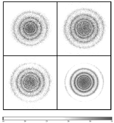
Figure 1.: Sample (logarithmic) power spectra as a function of $k_{x}$ and $k_{y}$ at a fixed frequency. The top panels are for the region centered at equator and Carrington longitude of $60^{\circ}$, at frequencies of around 3 mHz (left) and 4 mHz (right). The bottom left panel is the spectrum around 4 mHz for a region centered at $40^{\circ}$N latitude and longitude of $60^{\circ}$. The bottom right panel is the summed spectrum around 4 mHz for regions centered at the equator. The gray scale is marked with logarithm of the power.

To extract the flow velocities and other mode parameters from the 3d power spectra we fit a model of the form

$$P(k_{x},k_{y},\nu)={e^{B_{2}}\over k^{2}}+{e^{B_{3}}\over k^{3}}+\qquad\qquad\qquad$$ (1)

$$\qquad\qquad{\exp(A_{0}+(k-k_{0})A_{1}+A_{2}({k_{x}\over k})^{2}+A_{3}{k_{x}k_{y}\over k^{2}})\over(\nu-ck^{p}-U_{x}k_{x}-U_{y}k_{y})^{2}+w^{2}}$$

where $k^{2}=k_{x}^{2}+k_{y}^{2}$, and the 11 parameters $A_{0},A_{1},A_{2},A_{3},c,p,U_{x},U_{y},w,B_{2}$ and $B_{3}$ are determined by fitting the spectra using a maximum likelihood approach (Anderson et al. 1990). Here $k_{0}$ is the central value of $k$ in the fitting interval. The $A_{2}$ and $A_{3}$ terms account for the variation of power along the ring. The minimization has been performed using a quasi-Newton method based on the BFGS formula for updating the Hessian matrix (Antia 1991). The form given by Eq. (1) is slightly different from what is used by Patron et al. (1996), because we have assumed some variation in amplitude along the ring, coming from the $A_{2}$ and $A_{3}$ terms. These were introduced because the power does appear to vary along the ring and the fits in the absence of these terms were not satisfactory.

We fit each ring separately by using the portion of power spectrum extending halfway to the adjoining rings. For each fit we use a region extending about $\pm 100\mu$Hz from the chosen central frequency. We choose the central frequency for fit in the range of 2–5 mHz as the power outside this range is not significant. The rings corresponding to $0\leq n\leq 6$ have been fitted. This gives us typically 800 ‘modes’, all of them may not be independent as there is a considerable overlap between adjacent fitting intervals.

The fitted $U_{x}$ and $U_{y}$ for each mode represents an average over the entire region in horizontal extent and over the vertical region where the mode is trapped. We can invert the fitted $U_{x}$ (or $U_{y}$) to infer the variation in horizontal flow velocity $u_{x}$ (or $u_{y}$) with depth. We use the Regularized Least Squares (RLS) as well as the Optimally Localized Averages (OLA) techniques for inversion. For the purpose of inversion the fitted values of $U_{x}$ and $U_{y}$ are interpolated to the nearest integral value of $k$ (in units of $R_{\odot}^{-1}$) and then the kernels computed from a full solar model with corresponding value of degree $\ell$ are used for inversion.

We have selected the regions centered at Carrington longitudes of $90^{\circ},60^{\circ},30^{\circ}$ for rotation 1909 and at $360^{\circ},330^{\circ},300^{\circ}$ for rotation 1910 corresponding to period from about May 24 to June 7, 1996. For each longitude we select regions centered at latitudes of $0^{\circ}$, $\pm 10^{\circ}$, $\pm 20^{\circ}$, $\pm 30^{\circ}$, $\pm 40^{\circ}$, $\pm 50^{\circ}$ and $\pm 60^{\circ}$. There is some overlap between different regions. Apart from these individual spectra we have also analyzed spectra obtained by summing all 6 spectra for a given latitude to study the properties averaged over different longitudes. Because of averaging, these spectra have better statistics and the error estimates are also lower. These averaged spectra can be expected to give the average velocity over the range of longitudes considered. Most of the inferences in this work have been obtained using these averaged spectra. We fit each spectrum to obtain the mode parameters including $U_{x}$ and $U_{y}$.

3. RESULTS

Following the procedure outlined above we fit the form given by Eq. (1) to a suitable region of a 3d spectrum. Although other quantities may also be of some interest, in this work we restrict our attention to the two horizontal components of velocity (Fig. 2) obtained by fitting the spectra. The fitted velocities for each ‘mode’ are then inverted to obtain the variation of horizontal velocity with depth. Only the region $r>0.97R_{\odot}$ is sampled by the modes used in this study and hence the inversions are restricted to this region. Some of the results obtained using the RLS and OLA techniques are shown in Fig. 3.

Figure 2.: The fitted velocity for summed power spectra at different latitudes. In each panel the crosses mark the fitted velocity for northern hemisphere while the open squares mark that for the southern hemisphere. In the right panels the crosses marking northern latitudes generally fall in the upper half of the figure, while the squares marking southern latitudes fall in the lower half. The latitudes are marked in the left panel. Error bars are not shown for clarity.

Figure 3.: A sample set of inversions are shown for latitudes $\pm 40^{\circ}$ and longitude $300^{\circ}$. The circles and triangles are the OLA inversions for $40^{\circ}$N and $40^{\circ}$S respectively. The continuous and dashed lines are the RLS results for $40^{\circ}$N and $40^{\circ}$S respectively, with the dotted lines denoting the $1\sigma$ error limits.

From the inversion results it appears that the longitudinal component ($u_{x}$) is dominated by the average rotational velocity. This is a result of the fact that tracking is done at the surface rotation rate at the centre of the tracked region and hence does not account for the variation of the rotation rate with depth. The average variation with latitude, $\theta$ of these components can be determined from the summed spectra and a reasonable agreement between $u_{x}$ and the rotation rate determined from splitting coefficients of the global p-modes can be seen from Fig. 4. The rotation velocity at each latitude can be decomposed into the symmetric part [$(u_{N}+u_{S})/2$] and an antisymmetric part [$(u_{N}-u_{S})/2$]. The symmetric part can be compared with the rotation velocity as inferred from the splittings of global modes (Antia et al. 1998) and the results are shown in Fig. 5. Since the inversion results using global modes are not particularly reliable in the surface regions, the velocity profiles obtained from the ring diagram analysis supplement those results and support the earlier conclusions.

Figure 4.: The average horizontal velocity at different latitudes are compared with the rotation velocity (after subtracting out the surface rotation rate used in tracking each region) obtained from inversion of splitting-coefficients (continuous line). The results obtained using RLS inversions are shown by short-dashed (northern latitudes) and long-dashed lines (southern latitudes) with dotted lines marking the $1\sigma$ error limits. Similarly, the crosses (north) and squares (south) with error bars represent the results of OLA inversions.

Figure 5.: The average horizontal velocity at different latitudes (dashed line for RLS and crosses for OLA), i.e., the latitudinally symmetric part [$(u_{N}+u_{S})/2$], compared with the rotation velocity (after subtracting out the surface rotation rate used in tracking each region) obtained from inversion of splitting-coefficients (continuous line).

Following Kosovichev & Schou (1997) it is possible to decompose the rotation velocity into two components, a smooth part [polynomial in terms of $\cos(\theta)$, $\cos^{3}(\theta)$ and $\cos^{5}(\theta)$] and the remaining part which has been identified with zonal flows. The zonal flow so estimated is shown in Fig. 6. Despite poor latitudinal resolution in our results the inferred pattern near the surface is in reasonable agreement with the average zonal flow estimated from the splitting coefficients for the f-modes from the 360 day MDI data. But at deeper depths the pattern changes significantly and the errors are also larger. Hence, it is not clear if the zonal flow penetrates below about 7Mm ($0.01R_{\odot}$) from the surface.

Figure 6.: The zonal flow, i.e., the rotation velocity after removing a smooth component, at a layer just below the solar surface. The dotted line and points are RLS results, while the dashed line and points are OLA results. The error bars shown in this figure represent the error in rotation velocity and do not include any contribution from the smooth component which is subtracted to obtain these values. Hence the errors are likely to be underestimated. The continuous line represents the average zonal flow velocity as inferred from the f-modes using the 360 day MDI splitting coefficients.

Figure 7.: The antisymmetric component [$(u_{N}-u_{S})/2$] of the rotation velocity plotted as a function of depth for various latitudes. The lines are RLS and crosses are OLA results.

The difference between rotation velocity at the same latitude in the North and South hemispheres is small and thus the antisymmetric component of rotation rate is not very significant. Some of the difference may also be due to some systematic errors in our analysis. For example, due to differences in the angle of inclination for the regions at same latitude in the two hemisphere, the effect of foreshortening will be different in the two hemispheres. The antisymmetric component of the velocities is shown in Fig. 7. In particular, it can be seen that at low latitudes where the results are more reliable, the antisymmetric component is rather small, more or less within error estimates.

Figure 8.: Meridional velocity at different latitudes plotted as a function of depth. The results obtained using RLS inversions are shown by continuous lines (northern latitudes) and dashed lines (southern latitudes) with the dotted lines showing the $1\sigma$ error limits. Similarly, the crosses (north) in the positive half and squares (south) in the negative half of each panel represent the results of OLA inversions.

Figure 9.: Meridional velocity at different depths plotted as a function of latitude. These results have been obtained using the OLA technique for inversion.

The latitudinal component of the velocity appears to be dominated by the meridional flow from equator polewards. The average latitudinal velocity for each latitude is shown in Fig. 8, while Fig. 9 shows the same as a function of latitude at a few selected depths. There is a significant variation in this velocity with depth at high latitudes. Since the measurements are not particularly reliable at high latitudes it is difficult to say much about the general form of the flow velocity with latitude and moreover it will also depend on depth. However, if we fit to a form (cf., Giles et al. 1997)

$$u_{y}=a_{1}\cos(\theta)+a_{2}\cos(2\theta)$$ (2)

then we find mean flow $a_{2}$ of about 25–40 m/s depending on the depth, while $a_{1}$ is small, more or less comparable to error estimates. It is not clear if the assumed form indeed fits the measured variation as the resulting $\chi^{2}$ is fairly large. The expected decrease in the magnitude of $u_{y}$ at high latitudes, is not very clear from the results, though at layers immediately below the surface the meridional velocity does appear to decrease with latitude at high latitudes. The amplitude is about 25 m/s at a radial distance of $0.997R_{\odot}$ which is comparable to the estimated value obtained by Giles et al. (1997) from time-distance analysis and by Hathaway et al. (1996) from direct Doppler measurement at solar surface. The amplitude appears to increase rapidly with depth to about 40 m/s, and it is not clear if this form of latitudinal variation is actually valid at deeper depths where the velocity does not show any turnover at high latitudes. There is no evidence for any change in sign of the meridional velocity up to a depth of $0.03R_{\odot}$ or 21 Mm that is covered in this study.

Figure 10.: Horizontal flow velocities in horizontal planes at various depths obtained after the rotation and meridional velocities (as shown in Fig. 6 & 8) are subtracted from the individual measurements. The panels (a), (b), (c) and (d) respectively show the residual flow pattern at radial distance of 0.995, 0.990, 0.985 and $0.980R_{\odot}$ as inferred by the OLA inversion. The arrow at the top marks the scale. The errors in these measurements are not shown but they are typically 2–5 m/s depending on latitude and depth.

In order to extract other components of large scale flow fields and to study their variation with latitude and longitude we subtract out the average $u_{x}$ and $u_{y}$ as determined from the summed spectra, from those for individual regions. The residual velocities are shown in Fig. 10. Some of this velocity could be due to supergranules. It may be noted that the velocities at different longitudes in this figure gives the average values centered at different times. The rms residual velocity at each of these depths is found to be 12–16 m/s. There does not appear to be any clear pattern in this velocity thus suggesting that the giant cells if they exist have velocities less than about 10 m/s, or their life-time is smaller than the duration of about 15 days for which the data has been analyzed in this work, or their longitudinal (latitudinal) size is less than about $30^{\circ}$ ($10^{\circ}$).

4. CONCLUSIONS

The average longitudinal velocity agrees reasonably well with the rotation rate inferred from inversion of global p-modes. The zonal flow velocity in the outermost region also agrees with that estimated from the splitting coefficient for the global f-modes, though it is not clear if this flow continues in deeper layers. The antisymmetric component of the rotation velocity is small ($<5m/s$) and it is not clear if it is significant.

The dominant signal in the meridional velocity is the meridional flow which varies with latitude and has a maximum magnitude of about 40 m/s. The amplitude of meridional component increases from about 25 m/s just below the surface to 40 m/s in deeper layers. The form of variation with latitude is not very clear, but the velocity increases with latitude until about $40^{\circ}$ latitude at all depths. There is no change in sign of meridional velocity with depth up to 21 Mm.

The residual after removing the dominant rotation and meridional flow component has a magnitude of about 10 m/s and may represent flows due to the giant cells or some residual contribution from supergranules. From the absence of any clear pattern in these flows it appears that the giant cells if they exist have a velocities less than 10 m/s, or have lifetimes smaller than 15 days, or their longitudinal size is less than about $30^{\circ}$.

References

- \astronciteAnder1990 Anderson, E., Duvall, T., Jefferies, S., 1990, ApJ, 364, 699
- \astronciteAntia1991 Antia, H. M., 1991, Numerical Methods for Scientists and Engineers, Tata McGraw Hill, New Delhi
- \astronciteAntia1998 Antia H. M., Basu S., Chitre S. M., 1998, MNRAS (in press), astro-ph/9709083
- \astronciteBrumm1998 Brummell, N. H., Hurlburt, N. E., Toomre, J., 1998, ApJ, 493, 955
- \astronciteChoud1995 Choudhuri, A. R., Schussler, M., Dikpati, M., 1995, A&A, 303, L29
- \astroncitedurne1985 Durney, B. R., Cram, D. B., Guenther, S. L., Keil, D. M., Lytle, D. M., 1985, ApJ 292, 752
- \astronciteDuval1993 Duvall, T. L. Jr., Jefferies, S. M., Harvey, J. W., Pomerantz, M. A., 1993, Nature, 362, 430
- \astronciteGiles1997 Giles, P. M., Duvall, T. L. Jr., Scherrer, P. H., Bogart, R. S., 1997, Nature, 390, 52
- \astronciteHill1988 Hathaway, D. H., Gilman, P. A., Harvey, J. W. et al., 1996, Science, 272, 1306
- \astronciteHill1988 Hill, F., 1988, ApJ, 333, 996
- \astronciteHowar1996 Howard, R., 1996, ARA&A, 34, 75
- \astronciteKosov1997 Kosovichev, A. G. & Schou, J., 1997, ApJ, 482, L207
- \astroncitePatro1997 Patrón, J., Hernández, I. G., Chou, D.-Y., et al., 1997, ApJ, 485, 869
- \astronciteSchou1998 Schou, J., Antia, H. M., Basu, S., et al. 1998, ApJ, (in press)
- \astronciteSnodg1984 Snodgrass, H. B., Howard, R., 1984, ApJ, 284, 848
- \astronciteThomp1996 Thompson M. J., Toomre J., Anderson E. R., et al. 1996, Science, 272, 1300