A substructure analysis of the A3558 cluster complex

Abstract

The “algorithm driven by the density estimate for the identification of clusters” (DEDICA, Pisani 1993, 1996) is applied to the A3558 cluster complex in order to find substructures. This complex, located at the center of the Shapley Concentration supercluster, is a chain formed by the ACO clusters A3556, A3558 and A3562 and the two poor clusters SC 1327-312 and SC 1329-313. We find a large number of clumps, indicating that strong dynamical processes are active. In particular, it is necessary to use a fully three-dimensional sample (i.e. using the galaxy velocity as third coordinate) in order to recover also the clumps superimposed along the line of sight. Even if a great number of detected substructures were already found in a previous analysis (Bardelli et al. 1998), this method is more efficient and faster when compared with the use of a wide battery of tests and permits the direct estimate of the detection significance. Almost all subclusters previously detected by the wavelet analyses found in the literature are recognized by DEDICA.

On the basis of the substructure analysis, we also briefly discuss the origin of the A3558 complex by comparing two hypotheses: 1) the structure is a cluster-cluster collision seen just after the first core-core encounter; 2) this complex is the result of a series of incoherent group-group and cluster-group mergings, focused in that region by the presence of the surrounding supercluster. We studied the fraction of blue galaxies in the detected substructures and found that the bluest groups reside between A3562 and A3558, i.e. in the expected position in the scenario of the cluster-cluster collision.

1 Introduction

Clusters of galaxies are thought to form by accretion of subunits in a hierarchical bottom up scenario. This view arises naturally in various theories of cosmic structure formation, as f.i. the Cold Dark Matter dominated scenarios. Numerical simulations on scales of cosmological relevance (e.g. Cen & Ostriker 1994, Colberg et al. 1997) revealed that mergings happen along preferential directions, called density caustics, which define matter flows, at whose intersection rich clusters are formed. Detailed high resolution simulations of such collisions were performed by McGlynn & Fabian (1984) and Roettiger, Burns & Loken (1993), who studied cluster-cluster and cluster-group merging, respectively. In the simulations, the two cores have two or three encounters before dissipating all the kinetic energy: in particular, the less massive cluster emerges as a partially dispersed galaxy population along the down merger side of the dominant cluster. Members of the merging cluster, trapped nearby the dominant core, create an apparent clumpiness on either side of the center. The kinetic energy is dissipated mostly by the particles in external regions of the clusters, which expand creating a common envelope, while the cores do not change dramatically.

From the observational point of view, the detection of a large fraction of clusters which present substructures (see f.i. Kriessler & Beers 1997 and references therein) revealed that these systems are still dynamically young and show evidence of mergings. The best studied examples are A2256 (Briel, Henry & Böhringer 1992), where a small group is detected in the X-ray band nearby the cluster center, and Coma, where a number of substructures are revealed (Biviano et al. 1996). In particular, Burns et al. (1994), on the basis of the detection of a large scale X-ray emitting filament connecting Coma with the NGC4839 group, suggest that the group has probably already passed the cluster center.

The most spectacular phenomena are expected to be seen when the merging involves repeated collisions or even coalescence of comparable units: during the intermediate stages, the clusters form structures and complexes on scales of few megaparsecs.

Rich superclusters are the ideal environment for the detection of cluster mergings, because the peculiar velocities induced by the enhanced local density of the large scale structure favour the cluster-cluster and cluster-group collisions, in the same way as the caustics seen in the simulations. The most remarkable examples of cluster merging seen at an intermediate stage is found in the central region of the Shapley Concentration, the richest supercluster of clusters found within $300$  h^-1 Mpc (Zucca et al. 1993; hereafter h=H_o/100). On the basis of the two-dimensional distribution of galaxies of the COSMOS/UKSTJ catalogue (Yentis et al. 1992), it is possible to find several complexes of interacting clusters, which suggest that the entire region is dynamically active. Therefore, this supercluster represents a unique laboratory where it is possible to follow cluster mergings and to test related astrophysical consequences, as the formation of radio halos, relicts and wide angle tail radio sources and the presence of post-starburst (E+A) galaxies.

In this paper we perform a substructure analysis of the A3558 cluster complex using a non-parametric, scale independent algorithm, based on the adaptive kernel density estimator. This method could be considered alternative or complementary to the wavelet decomposition analysis, extensively used in literature. In particular, a wavelet analysis of this complex was done by Girardi et al. (1997) and, limited to the dominant cluster A3558, by Dantas et al. (1997): these analyses offer an opportunity to test the two methods on a real, rather complex situation. In Section 2 we briefly describe the method, in Section 3 the used samples are presented and in Section 4 a brief discussion of the subclumps is reported; finally in Section 5 we present our conclusions.

2 The method

In order to identify the substructures in our sample and to assess their significance, we followed the method known as “algorithm driven by the density estimate for the identification of clusters” (hereafter DEDICA) developed by Pisani (1993, 1996). This is a non-parametric, scale independent method, whose output gives a list of groups with the related statistical significance, their members, and a list of isolated objects. Here we remind briefly the main steps of the method.

First, we estimated the density field $f(\vec{x})$ (where $\vec{x}$ is the $n$-dimensional position vector) using the “adaptive kernel probability estimator” for which

$$f_{k}(\vec{x})={1\over N}\sum^{N}_{i=1}K(\vec{x}_{i},\sigma_{i};\vec{x})$$ (1)

where $f_{k}(\vec{x})$ is the kernel estimator of $f(\vec{x})$, $\vec{x}_{i}$ is the position of the $i^{th}$ galaxy, $N$ is the number of objects in the sample and $\sigma_{i}$ is the size of the gaussian kernel defined as

$$K(\vec{x}_{i},\sigma_{i};\vec{x})={1\over{\left(2\pi\sigma_{i}^{2}\right)^{d/2}}}exp\left(-{{|\vec{x}_{i}-\vec{x}|^{2}}\over{2\sigma_{i}^{2}}}\right)$$ (2)

where $d$ is the number of dimensions of the sample.

We stress that we choose the Gaussian form for the kernel basically because it is differentiable in all its domain. This is a crucial feature in order to identify the density peaks according to Eq. 7. Even if the most efficient (i.e. with minimum variance) kernel form is the Epanechnikov function, Silverman (1986) showed that difference in the use of the two forms is negligible. Indeed, what is crucial for cluster detection is the width and not the shape of the kernels, provided that they satisfy the normalization and convergence condition (see section I of Pisani 1993).

The estimate of the kernel sizes is done through an iterative procedure, starting from a large value for the kernel sizes and progressively reducing them until the minimum of the “cross-validation function” is reached. The various steps are the following (for details see Pisani 1993, 1996):

1) set the first guess ($n=0$) of the size as $\sigma_{0}=4\sigma_{t}$ where

$$\sigma_{t}=0.96N^{[-1/(d+4)]}\sqrt{{1\over d}\sum^{d}_{l=1}s_{l}^{2}}$$ (3)

where $s_{l}^{2}$ is the standard deviation of the $l^{th}$ coordinate (Silverman 1986). In this step, a large starting $\sigma_{0}$ is selected: note that for a symmetric gaussian distribution with dispersion $\sigma_{G}$ and same number of points of our samples, we have $\sigma_{0}\sim 1-1.5\sigma_{G}$;

2) set the following iteration ($n^{th}$) as $\sigma_{n}=\sigma_{n-1}/2$;

3) take as “pilot function” $f_{p}(\vec{x})$ the density kernel estimate $f_{k}(\vec{x})$ with sizes $\sigma_{i}$ fixed at $\sigma_{n}$ $\forall i$ (see eq. 27 and 28 of Pisani 1993);

4) set $\sigma^{\prime}_{i}=\lambda_{i}\sigma_{n}$, where $\lambda_{i}$ is a “local bandwidth” defined as

$$\lambda_{i}=\left({{f_{p}(\vec{x}_{i})}\over{g}}\right)^{-0.5}$$ (4)

where

$$\log\ g={1\over N}\sum_{i=1}^{N}\log(f_{p}(\vec{x}_{i}))$$ (5)

Now, the sizes of the kernels $\sigma^{\prime}_{i}$ are depending somehow from the local density through the factor $\lambda_{i}$: the higher is the density, the smaller are the $\sigma^{\prime}_{i}$;

5) evaluate the cross-validation function $CV[f_{k}](\sigma_{n})$ of the $n^{th}$ estimate of the density $f_{k}$ (eq. 4 and 5 of Pisani 1996). The $CV[f_{k}](\sigma_{n})$ estimates the quadratic deviation between $f_{k}(\vec{x})$ and the “true” parent density function $f(\vec{x})$ (see eq. 33 of Pisani 1993).

The steps from (2) to (5) are iterated until the minimum of $CV[f_{k}](\sigma_{n})$ is reached: the corresponding kernel widths $\sigma^{\prime}_{i}$ give the optimal density estimate $\hat{f}_{k}(\vec{x})$ as:

$$\hat{f}_{k}(\vec{x})={1\over N}\sum^{N}_{i=1}K(\vec{x}_{i},\sigma^{\prime}_{i};\vec{x})$$ (6)

Peaks in the density distribution function are assumed to define the presence of clusters (in this section we use the word cluster in the statistical sense): the local maxima of $\hat{f}_{k}(\vec{x})$ are found by solving for each starting $i^{th}$ galaxy position ($i=1,N$) the iterative equation

$$\vec{x}_{m+1,i}=\vec{x}_{m,i}+{d\over{\sum^{N}_{i=1}\left(\displaystyle{{{\nabla\hat{f}_{k}(\vec{x}_{m,i})}\over{\hat{f}_{k}(\vec{x}_{m,i})}}}\right)^{2}}}\left({{\nabla\hat{f}_{k}(\vec{x}_{m,i})}\over{\hat{f}_{k}(\vec{x}_{m,i})}}\right)$$ (7)

where $\vec{x}_{1,i}$ is the original position of the $i^{th}$ galaxy. Eq. (7) defines a path from the original position to a limiting point along the maximum gradient of the function $\hat{f}_{k}(\vec{x})$ All starting points which reach the same limiting position $\vec{x}_{lim}$ for $m\to\infty$ define a cluster. From the analysis of the distribution of the distances between the various $\vec{x}_{lim}$ in our samples, we decided to consider coincident all the limiting points that differ by less than $0.1$ arcmin.

The significance of the cluster is estimated by calculating first the likelihood function of the sample

$$L=\prod_{i=1}^{N}f_{k}(\vec{x}_{i})=\prod_{i=1}^{N}\sum_{\mu=0}^{\nu}F_{\mu}(\vec{x}_{i})$$ (8)

where $F_{\mu}(\vec{x}_{i})$ is the contribution to the density function of the $\mu^{th}$ cluster $C_{\mu}$, calculated as

$$F_{\mu}(\vec{x})={1\over N}\sum_{j\in C_{\mu}}K(\vec{x}_{j},\sigma_{j};\vec{x})$$ (9)

where the sum is done on the galaxies belonging to the $\mu^{th}$ cluster and $\nu$ is the number of clusters found in the sample. For $\mu=0$ we refer to the set of isolated galaxies, i.e. those that did not reach a $\vec{x}_{lim}$ shared with other object.

Then the likelihood of the $\mu^{th}$ cluster ($L_{\mu}$) is calculated by replacing in Eq. (8) the sizes $\sigma^{\prime}_{i}$ of the kernels of the substructure objects with $\sigma_{bck}$, i.e. the kernel size of the background. The ratio $\chi^{2}=\displaystyle{-2\ln{L_{\mu}\over L}}$ is distributed as a chi square variable with one degree of freedom and is related to the probability that the density distribution is better described by the presence of the $\mu^{th}$ cluster rather than by a uniform background.

In an ideal case, it would be possible to determine $\sigma_{bck}$ by using the isolated galaxies, because they are likely to be part of the background. However, also local fluctuations of the density field of a cluster can be identified as local maxima and hence this fact causes a misidentification of cluster members as isolated galaxies.

A method to identify really isolated galaxies is to check the relative contribution to the total density of the kernel of the $i^{th}$ galaxy in the position $\vec{x}_{i}$ (Pisani 1996), given by

$$P(i\in C_{0})={1\over N}{{K(\vec{x_{i}},\sigma_{i};\vec{x_{i}})}\over{\hat{f}_{k}(\vec{x})}}$$ (10)

This equation estimates the probability that a “nominally” isolated galaxy is really part of the background. We found that for our samples $P(i\in C_{0})\leq 0.15$, hence we can conclude that there are no really isolated galaxies. Note that the estimate of $P(i\in C_{0})$ is independent from the cluster identification step (Eq. 7).

In order to determine a value for the background, we plotted the histogram of the kernel sizes $\sigma^{\prime}_{i}$, which is a symmetric distribution with a tail at higher values. We choose as $\sigma_{bck}$ the value at the beginning of the tail (see Fig. 2a in Sect. 3.1).

The group significances calculated from the values of $\chi^{2}$ are strictly correct only if the background is well determined, that is not our case. For this reason we regard the $\chi^{2}$ only as a ranking parameter for the existence of the groups and we consider only subclusters in the tail at higher values of this parameter (see Fig. 2b in Sect. 3.1). This choice corresponds approximately to a “formal” significance of $99.9\%$. We forced the background at various reasonable densities in order to check the robustness of our results, finding that the general clustering pattern of our samples is not strongly dependent on the poorly known global background density.

As a test of the efficiency of this method, we applied DEDICA to simulated Gaussian distributions, where no substructures are expected. We performed various simulations of 2-D and 3-D Gaussians, with a number of points between 300 and 700 (which are the approximate numbers of galaxies in our various samples), finding that the success rate (i.e. absence of significant substructures) of DEDICA is always between $80\%$ and $90\%$ (depending on the number of objects). In the cases in which DEDICA finds significant substructures, the numbers of these “spurious” groups is of the order of 2-3.

This method differs from the wavelet decomposition because it is non-parametric and scale-independent. Indeed, the wavelet method is a deconvolution procedure, which assumes an exploring function, which is fixed throughout the whole sample volume. On the contrary, DEDICA adopts a kernel function, which is locally density dependent and in this sense is not a deconvolution method (Silverman 1986). The wavelet analysis is able to detect structures depending on the scale of the exploring function, while DEDICA does not requires any assumption on the scale of clusters.

3 The A3558 cluster complex

In a series of papers (Bardelli et al. 1994, 1996, 1998, hereafter Paper 1, 2 and 3; Venturi et al. 1997) we performed a detailed multiwavelength study of the A3558 cluster complex, a remarkable association formed by three ACO (Abell, Corwin & Olowin 1989) clusters A3556, A3558 and A3562, already noticed by Shapley (1930). This structure is approximately at the geometrical center of the Shapley Concentration and can be considered the core of this supercluster. By the use of multifibre spectroscopy, we obtained 714 redshifts of galaxies in this region, confirming that the complex is a single connected structure, elongated perpendicularly to the line of sight. In particular, the number of measured redshifts of galaxies belonging to A3558 is $307$, and thus this is one of the best sampled galaxy clusters in the literature. Moreover, two smaller groups, dubbed SC 1327-312 and SC 1329-313, were found both in optical (Paper 1) and X-ray band (Breen et al. 1994; Paper 2). In particular, in Paper 2 we detected a bridge of X-ray emitting hot gas connecting A3558 and SC 1327-313 (and possibly extending to A3562, see figure 7 of Ettori et al. 1997) which resembles the structure between Coma and NGC4839 described by Burns et al. (1994). The presence of this feature strongly supports the suggestion by Metcalfe et al. (1994) that A3562 already encountered A3558: the bridge could be the tail of gas left by A3562 after the first passage through A3558 (for details see Burns et al. 1994).

The clusters of this complex attracted the attention of various investigators, who applied several statistical tests in order to detect substructures. Bird (1993), applying both 2-D and 3-D tests to galaxies in A3558, found three subclumps: the first coincides with the cluster center and corresponds to the main component, the second lies eastward of the cluster center and the third is in the south-east quadrant.

In Paper 3, applying the test developed by Dressler & Shectman (1988), we detected a group at $\sim 10$ arcmin from the position of the second clump of Bird (1993). From the analysis of the isodensity contours and the velocity distribution histograms, there was evidence of another density excess at $\sim 15$ arcmin southward of the A3558 center. Moreover, A3558, SC1329-313 and A3556 appear to have bimodal velocity distributions.

Girardi et al. (1997), using a modified version of the bi-dimensional wavelet decomposition which takes into account also the dynamical information, individuated in A3558 the same subclumps found by Bird (1993) and by us (Paper 3), and an additional substructure westward of the center of A3562.

Dantas et al. (1997), using the bi-dimensional wavelet decomposition in A3558, detected a bimodality in the core of the cluster. The authors claim that this result resolves both the cD offset problem (in fact the dominant galaxy was suspected not to be at rest with respect to the cluster velocity centroid, Gebhardt & Beers 1991), and the “$\beta$ problem” (Paper 2), by decreasing the central velocity dispersion from $\sim 1000$ km/s to $\sim 800$ km/s

Analysing a ROSAT PSPC image of A3558, we noted (Paper 2) that the diffuse emission of the hot gas is better described by two components, one centered on the geometrical center of the cluster and the other on the cD galaxy. Slezak et al. (1994) applied the wavelet analysis to this X-ray map and found evidence of a substructure nearby the cluster core.

Table 1: Groups in the bi–dimensional sample

#	$\alpha$ (2000)	$\delta$ (2000)	# mem.	# vel.	$<v>$	$\sigma$	notes
B109	13 22 31.4	-31 18 22	34				A5556
B194	13 22 57.7	-31 37 46	67	14	14360${}^{+117}_{-145}$	520${}^{+115}_{-68}$	A3556
B353	13 24 15.4	-31 40 40	46	22	14492${}^{+131}_{-164}$	575${}^{+86}_{-44}$	A3556
B694	13 26 58.3	-31 21 29	57	20	14038${}^{+151}_{-224}$	771${}^{+106}_{-138}$	A3558
B830	13 27 07.2	-31 51 53	72	26	14728${}^{+147}_{-178}$	674${}^{+181}_{-173}$	A3558
B906	13 27 52.0	-31 29 23	81	52	14501${}^{+125}_{-183}$	1001${}^{+119}_{-80}$	A3558
B1000	13 28 04.0	-31 44 41	55	24	13813${}^{+136}_{-286}$	947${}^{+112}_{-78}$	A3558
B1014	13 28 05.8	-31 05 24	24				A3558
B1056	13 28 07.4	-31 33 05	53	29	14064${}^{+112}_{-282}$	991${}^{+178}_{-122}$	A3558
B1199	13 29 00.5	-31 49 23	51	18	14728${}^{+259}_{-279}$	971${}^{+122}_{-189}$	A3558
B1311	13 29 23.7	-31 21 34	57	23	15029${}^{+228}_{-375}$	1081${}^{+135}_{-168}$	A3558
B1443	13 30 28.0	-31 36 41	100	37	14652${}^{+182}_{-149}$	842${}^{+150}_{-56}$	Poor
B1573	13 31 08.2	-31 46 58	111	49	14059${}^{+116}_{-257}$	1051${}^{+160}_{-53}$	Poor
B1952	13 33 28.1	-31 41 16	179	35	14447${}^{+230}_{-305}$	1113 ${}^{+103}_{-112}$	A3562
B2103	13 34 50.8	-31 40 14	37	8	14751${}^{+156}_{-502}$	880${}^{+396}_{-107}$	A3562
B2240	13 35 38.3	-31 55 40	76	18	14343${}^{+445}_{-100}$	1462${}^{+445}_{-100}$	A3562

3.1 The bi–dimensional sample

From the COSMOS/UKST galaxy catalogue (Yentis et al. 1992), we extracted a rectangular region of $3^{o}.2\times 1^{o}.4$, corresponding to $13^{h}22^{m}06^{s}<\alpha(2000)<13^{h}37^{m}15^{s}$ and $-32^{o}22^{\prime}40^{\prime\prime}<\delta(2000)<-30^{o}59^{\prime}30^{\prime\prime}$. This region is part of the UKSTJ plate $444$ and contains the A3558 complex. We restricted our analysis to the $2241$ galaxies with magnitudes brighter than $b_{J}=19.5$. The isodensity contours of galaxies of this region are presented in Fig. 1.

Figure 1: Galaxy isodensity contours of the region of the A3558 cluster complex: the objects are binned in $2$ arcmin $\times$ $2$ arcmin pixels and then smoothed with a Gaussian with a FWHM of $6$ arcmin. Dashed lines correspond to 1 Abell radius circles around cluster centers. The positions of the two poor clusters SC 1327-312 and SC 1329-313 are shown.

The adopted $\sigma_{bck}$ is 6.4 arcmin, which corresponds to $0.05$ gal arcmin^-2, and a $\chi^{2}$ threshold of 12 (Fig. 2).

The DEDICA algorithm found 113 groups, 16 of which are considered significant. In Table 1 the 16 significant clusters sorted by right ascension are listed. Column (1) is the identification number while columns (2) and (3) give the $\alpha$ and $\delta$ coordinates of the group center. We identified these points as the common $\vec{x}_{lim}$ position of the members and they do not necessarily coincide with the geometrical centers. Columns (4) and (5) report the number of the cluster members and of the available velocities in the group. Columns (6) and (7) are the dynamical parameters computed using the biweight estimators of position and scale (see Paper 1 for details on the method). Finally, Column (8) reports the main component to which the substructures belong, i.e. the A3556, A3562, A3558 Abell clusters, and the poor clusters SC 1317-312 and SC1329-313 (denoted as “Poor”).

The velocity sample (see below) covers an area which is $\sim 17\%$ of the bi-dimensional sample and therefore not all subclusters have measured velocities: for this reason in two cases the dynamical parameters are left blank in Table 1.

Figure 2: a) Histogram of the kernel sizes $\sigma^{\prime}_{i}$ for the bi–dimensional sample. The vertical dashed line corresponds to the adopted $\sigma_{bck}=6.4$ arcmin. b) Histogram of the $\chi^{2}$ values for the detected groups in the bi–dimensional sample. The vertical dashed line corresponds to the adopted threshold of significance ($\chi^{2}=12$).

3.2 The three–dimensional sample

In this case we used the velocity sample described in Paper 3. From the $714$ galaxies with measured redshift we selected the $600$ objects in the velocity range $[10000-20000]$ km/s. The velocity sampling of the A3558 complex is not constant: it varies from $\sim 20\%$ in the region of A3562 to $\sim 48\%$ in the core of A3558. This fact could cause a bias that erases undersampled substructures or leads to false detections in regions more sampled than the average.

In order to check this point, we performed the bi-dimensional analysis on this subsample. Among the 14 bi-dimensional groups present in the area of the velocity sample, 13 are correctly detected and $B2240$ (corresponding to T599) has been lost because of a significance lower than the limit. The tight correspondence between bi-dimensional and these “three-dimensional” groups indicates that this bias is not severe.

Given the fact that the velocities are not related to positions because of the dominance of peculiar motions over the Hubble flow, a problematic point is how to handle the velocity coordinate. Our formalism uses symmetric three-dimensional gaussian kernels, with $\sigma_{x}=\sigma_{y}=\sigma_{v}$ and therefore it is necessary to scale the velocity interval in order to have a numerical range comparable to the other two variables. The typical $\sigma$ of the spatial coordinates is 2-3 arcmin, while the typical $\sigma_{v}$ (determined on the one-dimensional redshift distribution) is $\sim 200$ km/s. We have therefore chosen to compress the velocity by a factor 100; we have also checked that the method gives essentially the same results if this reduction factor is in the range $50-500$.

A more precise approach to this problem requires the modelling of the peculiar velocity field. This implies the detailed knowledge of the mass distribution in the A3558 complex, which is presently not available. In fact there is no general agreement even for the mass of the dominant, best studied, cluster of the complex (A3558). The mass obtained from optical data ranges from $3.4\times 10^{14}$ h^-1 M_⊙ (Dantas et al. 1997) to $6\times 10^{14}$ h^-1 M_⊙ (Biviano et al. 1993), while the X-ray data give mass in the range $1.5-6.0\times 10^{14}$ h^-1 M_⊙ (Paper 2, Ettori et al. 1997).

The adopted value of the background is $\sigma_{bck}=7.5$ arcmin, corresponding to 0.003 gal arcmin^-2 (km/s/100)^-1 and a significance threshold of $\chi^{2}=20$. The significant 3-D clusters are $21$, out of a total of $36$, and are reported in Table 2. Column (1) is the subcluster identification number, Columns (2), (3) and (4) report the coordinates ($\alpha$, $\delta$ and $v_{o}$) of the group center, while the number of members is reported in Column (5). The estimated dynamical parameters are reported in Columns (6) and (7) and in Column (8) the general position is given. Note that in some cases, the velocity distributions are highly asymmetric and therefore there is a significant difference between $v_{o}$ (the position of the density peak) and the mean velocity estimated with the biweight method.

In Figs. 3, 5, 7 and 9 the positions of the substructure members are shown, superimposed on the isodensity contours of galaxies obtained with a smoothing of $2$ arcmin. Note that in these figures the isodensity contours are obtained directly by binning the data in one arcmin cells and not from the $\hat{f}_{k}$: however the two methods give similar contours. In Figs. 4, 6, 8 and 10, the groups members are shown projected on the X-Velocity plane. Solid lines connect the position of each galaxy to the common limiting position $\vec{x}_{lim}$ of the group.

Table 2: Three–dimensional sample

#	$\alpha$ (2000)	$\delta$ (2000)	$v_{0}$	# mem.	$<v>$	$\sigma$	notes
T17	13 23 03.0	-31 43 37	14501	12	14498${}^{+83}_{-117}$	334${}^{+124}_{-55}$	A3556
T49	13 23 42.7	-31 49 23	14366	21	14173${}^{+104}_{-125}$	410${}^{+68}_{-69}$	A3556
T75	13 23 59.0	-31 39 57	15075	19	15087${}^{+28}_{-71}$	154${}^{+34}_{-34}$	A3556
T96	13 24 23.9	-31 41 14	14129	32	14035${}^{+58}_{-125}$	397${}^{+61}_{-46}$	A3556
T194	13 26 56.9	-31 22 34	14139	24	13721${}^{+172}_{-111}$	625${}^{+178}_{-52}$	A3558
T260	13 26 59.0	-31 54 46	14715	34	14605${}^{+109}_{-88}$	622${}^{+134}_{-133}$	A3558
T337	13 27 50.9	-31 28 48	13903	45	13597${}^{+90}_{-210}$	693${}^{+163}_{-40}$	A3558
T281	13 27 53.3	-31 30 47	15420	22	15456${}^{+83}_{-56}$	294${}^{+68}_{-39}$	A3558
T301	13 27 57.9	-31 44 35	13416	21	13224${}^{+113}_{-152}$	500${}^{+75}_{-67}$	A3558
T300	13 28 00.1	-31 35 08	14952	22	14876${}^{+53}_{-82}$	242${}^{+46}_{-36}$	A3558
T338	13 28 19.8	-31 31 31	14195	22	14213${}^{+63}_{-93}$	345${}^{+56}_{-14}$	A3558
T359	13 28 58.2	-31 48 57	15463	13	15393${}^{+175}_{-187}$	788${}^{+211}_{-202}$	A3558
T413	13 29 19.9	-31 23 16	15088	34	15392${}^{+121}_{-151}$	691${}^{+110}_{-41}$	A3558
T478	13 30 10.8	-31 36 29	15154	26	15069${}^{+80}_{-162}$	515${}^{+125}_{-70}$	Poor
T441	13 30 33.4	-32 03 59	13025	11	12948${}^{+41}_{-52}$	159${}^{+276}_{-89}$	Poor
T496	13 30 52.3	-31 50 01	14663	38	14690${}^{+101}_{-99}$	537${}^{+87}_{-32}$	Poor
T520	13 31 12.8	-31 46 29	13437	42	13280${}^{+80}_{-95}$	482${}^{+87}_{-49}$	Poor
T514	13 32 26.7	-31 02 58	13543	5	13510${}^{+248}_{-152}$	287${}^{+83}_{-24}$	Poor
T561	13 33 31.6	-31 35 19	14501	30	14527${}^{+168}_{-229}$	987${}^{+116}_{-67}$	A3562
T598	13 34 58.6	-31 38 59	14981	18	14867${}^{+318}_{-231}$	919${}^{+149}_{-141}$	A3562
T599	13 35 33.6	-31 54 24	14426	14	14412${}^{+111}_{-50}$	278${}^{+106}_{-42}$	A3562

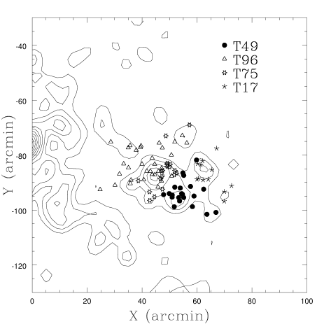
Figure 3: Groups in the A3556 cluster region. The positions of sub-cluster galaxies found in the three-dimensional sample are overplotted to the 2-D isodensity contours smoothed with a 2 arcmin FWHM Gaussian. Symbols used to label the different groups are explained in the figure.

Figure 4: Projection on the X-Velocity plane of groups in the A3556 cluster region. Solid lines connect the position of each galaxy to the common limiting position $\vec{x}_{lim}$ of the group.

Figure 5: The same as Fig. 3, for groups in the A3558 cluster region. For clearness the group members have been split in two panels

Figure 6: The same as Fig. 4 for groups in the A3558 cluster region.

4 Results and discussion

4.1 A3556

The bi-dimensional analysis found $2$ significant groups in the inner part of this cluster, being the substructure $B109$ at about one Abell radius from the center. The distribution of galaxies is not smooth as can be seen also in Fig. 3, where the isodensity contours show three peaks. However, the dynamical analysis of the substructures reveals that mean velocities and velocity dispersions are consistent with the values of $<v>=14357^{+76}_{-76}$ km/s and $\sigma=643^{+53}_{-43}$ km/s given in Paper 3 for the whole cluster.

The three-dimensional analysis shows four subclumps: two of them ($T49$ and $T96$) have dynamical parameters consistent each other at about one sigma and correspond to two nearby ($\sim 12$ arcmin) density maxima separated on the plane of the sky.

The group $T75$ appears superimposed along the line of sight with $T96$ (they correspond to $B353$), but at higher velocity: the presence of these two peaks in the redshift distribution was already detected in Paper 3, with consistent dynamical parameters. Moreover, as noted by Venturi et al. (1997, 1998), $T75$ contains the head-tail radiosource $J1324-3138$: the head-tail appearance of this source could indicate an interaction with a gaseous medium during the infall of the group toward the main clump of A3556.

The group $T17$ seems to be at an intermediate mean velocity and separated in the plane of sky from the other clumps. The westernmost galaxy of this group (well outside the density peak) corresponds to the Wide Angle Tail radio source studied by Venturi et al. (1997). In the bi-dimensional analysis this object is associated to $B109$, but also in this case it is at the edge of the substructure. This fact is anomalous for Wide Angle Tail sources, found normally at the center of clusters or groups (Owen 1996).

In conclusion A3556, which appears at a first look as a relatively relaxed cluster (see figures 1 and 2 of Paper 3), revealed after a more detailed analysis a relevant clumpiness in its core. This is an indication that the dynamical processes have not had enough time to destroy the substructures and to smooth the galaxy distribution.

4.2 A3558

The bi-dimensional analysis revealed that the inner core ($r<0.75$  h^-1 Mpc ) of this cluster could be separated in two groups: $B906$, which contains the dominant galaxy, and $B1056$. This spatial bimodality was already found by Dantas et al. (1997) using the bi-dimensional wavelet analysis: the positions of their clumps A and B differ only by $\sim 1$ arcmin from our groups and there is a good consistency in the dynamical parameters. However, the three-dimensional analysis shows that the situation is more complex, with four subclusters ($T337$, $T281$, $T300$ and $T338$) almost aligned along the line of sight. In particular, the bi-dimensional group $B906$ is broken into two components, at $<v>=15456$ km/s ($T281$) and $<v>=13597$ km/s ($T337$): note that the mean velocity of $T281$ is consistent with that of clump A^′ of Dantas et al. (1997).

The main three-dimensional structure is the group $T337$. The group $T194$ has similar dynamical parameters and could therefore be considered an elongation of $T337$. Merging these two clumps together in order to have a larger sample, we find $<v>=13640^{+78}_{-124}$ km/s and $\sigma=665^{+86}_{-69}$ km/s. We are consistent with the results found by Bird (1994), Girardi et al. (1997) and Dantas et al. (1997) that the velocity dispersion of the main component of $A3558$ is of the order of $\sim 700$ km/s. This velocity dispersion is more consistent with the lower X-ray temperature found by ROSAT ($3.25$ keV Paper 2), rather than the higher temperature detected by ASCA ($5.5$ keV, Markevitch & Vikhlinin 1997). The velocity histogram of $T337+T194$ is asymmetric with a tail toward low velocities: the peak of the distribution is located at $\sim 14100$ km/s, a value consistent with the cD velocity.

The bi-dimensional clump $B1000$ has a positional coincidence in the plane of the sky with $T301$. These structures are located on a density excess, southward of the cluster center, already noted in Paper 3 and detected by the use of the West et al. (1988) symmetry test. This density excess was revealed also by the presence of two peaks in the velocity distribution in the third radial shell of Paper 3. The dynamical parameters of the lower velocity peak are well consistent with those of $T301$, while the higher velocity peak is probably associated to galaxies of group $T413$ which also fall in this shell. The latter clump has been detected by Bird (1994), Girardi et al. (1997) and in Paper 3 using the Dressler & Shectman (1988) $\Delta$ test. As noted in Paper 3, this substructure is in the region of A3558 which show a significant enhancement of temperature (Markevitch & Vikhlinin 1997).

Another relevant condensation is the group $T260$ (or $B830$), in the south-west part of A3558, whose isodensity contours appear elongated.

4.3 SC1327-312 and SC1329 -313

An interesting feature of the A3558 complex is the presence of a number of clumps between A3558 and A3562, which form a series connecting the two clusters, starting with $T413$ and $T359$ just on the east of A3558. In the X-ray band there are two relevant diffuse emissions dubbed SC 1327-312 and SC 1329-314 (Breen et al. 1994; Paper 2) already noted also in the optical band (Paper 1). The SC 1327-312 group probably corresponds to $T478$, even if there is an offset of $\sim 5$ arcmin between the two positions. In Paper 3 we noted a bimodality in the velocity distribution of SC 1329-313: these two groups are recovered as $T520$ and $T496$.

Figure 7: The same as Fig. 3, for groups in the Poor clusters region.

Figure 8: The same as Fig. 4 for groups in the Poor cluster region.

4.4 A3562

From the analysis of the three-dimensional sample it is possible to find out three components. The main cluster component appears to be $T561$, with a velocity dispersion of $\sim 900$ km/s, consistent with that found in Paper 3. Note the presence of other two clumps ($T599$ and $T598$) probably connected with the main cluster.

5 Conclusions and Discussion

The DEDICA algorithm is a non-parametric, scale independent method for substructure analysis. We used this algorithm on both a bi-dimensional and a three-dimensional (i.e. using the galaxy velocity as third coordinate) sample in the region of the A3558 complex. The bi-dimensional analysis finds a large number of clumps in correspondence of evident density peaks, but it appears insufficient to correctly characterize all the substructures: in fact the three-dimensional analysis finds several cases in which different subclumps aligned along the line of sight are seen as single bi-dimensional peaks.

On the other hand, the not uniform and incomplete sampling in velocity may in principle lead to miss some structures in the three-dimensional analysis. However, this incompleteness does not seem to introduce significant artifacts, because there is a good correspondence between the three-dimensional subcluster centers and most of the bi-dimensional density excesses.

A number of these subclusters were already detected in Paper 3 by the simultaneous use of various techniques, such as the classical shape estimators, the West et al. (1988) and the Dressler & Shectman (1988) tests and the analysis of the velocity histograms with the KMM algorithm (Ashman, Bird & Zepf 1994). The efficiency of these methods depends on the properties of the substructures: for example, the West et al. test recovers groups as departures from the mirror symmetry of the main cluster, while the Dressler & Shectman method is insensitive to subclusters which are superimposed along the line of sight or with similar mean velocity and velocity dispersion. This fact led Pinkney et al. (1996) to recommend for the substructure analysis of clusters the use of a wide battery of statistical tests. Under this aspect, the DEDICA algorithm is more efficient and faster and permits a direct estimate of the significance of the detected clump, without relying on long computer simulations.

A direct comparison with the results obtained with the wavelet decomposition analysis is not straightforward because of the different starting samples. The subclusters detected by Girardi et al. (1997) are a subset of our sample, revealing that the two methods are similar as discussed by Fadda et al. (1998). The difference in the dynamical parameters are probably due to the fact that the method of Girardi et al. is not fully three-dimensional. Our bi-dimensional analysis of the center of A3558 gives the same results of Dantas et al. (1997), i.e. the inner 0.5 Abell radius region is formed by two clumps, one of which ($B906$) approximatively centered (within $\sim 1$ arcmin) on the X-ray excess of the cD galaxy. On the contrary, our three-dimensional analysis reveals a more complicated situation.

Figure 9: The same as Fig. 3, for groups in the A3562 cluster region.

Figure 10: The same as Fig. 4 for groups in the A3562 cluster region.

It is possible to consider two main hypotheses for the origin of the A3558 cluster complex: one is that we are observing a cluster-cluster collision, just after the first core-core encounter, while the other considers repeated, incoherent group-group and group-cluster mergings focused at the geometrical center of a large scale density excess (the Shapley Concentration).

In the first scenario, we could speculate that a cluster collided onto A3558 and its remnants are visible as the overdensity regions of SC 1327-312, SC1329-313 and A3562: the connection of hot gas between A3558 and SC1327-312 found in Paper 2 could be a trace of such a collision. In this framework, A3556 would be formed by the members of the intervening cluster remained in the backside part of the merging direction. Therefore, galaxies outside A3558 would belong to the destroyed cluster and to the outer regions of the more massive target cluster and form the clumpiness expected in the simulations.

Caldwell & Rose (1997) suggested that the infall of a group onto a cluster may trigger starburst phenomena on its galaxies. Indeed they found a number of objects showing recent star formation in the filament connecting the Coma cluster with NGC4839, which was suspected by Burns et al. (1994) to have already passed the core of Coma. In order to check if the cluster interaction modifies the galaxy spectral emission, we cross-correlated our velocity sample with the photometric sample of Metcalfe et al. (1994), which contains $B$ magnitudes and the $(U-B)$, $(B-R)$ and $(R-I)$ colours to $B=20.8$. The use of the velocity sample, limited in the $[10000-20000]$ km/s range, eliminates the ambiguity of possible colour effects due to objects at various redshifts. We consider “blue galaxies” those with $(U-B)<0.3$: this choice should allow to exclude the “red sequence” in the colour-magnitude planes typical of the presence of clusters and to have at the same time a large number of objects (157) in the blue sample.

Dividing the galaxies into two groups, i.e. those that are in significant groups and those that are outside them, we found that the fractions of blue objects are $25\%$ and $45\%$, respectively. The reddest group is $T337$ with a fraction of $5\%$ of blue galaxies and this supports the idea that the group could be considered as a preexisting, already relaxed cluster (that is A3558). The bluest groups are $T520$ and $T441$ with $47\%$ and $45\%$ of blue galaxies and are in the expected position in the scenario of a cluster-cluster collision, i.e. between A3562 and A3558.

In the second scenario, instead of a single merging phenomenon, there would have been a series of minor mergings and collisions, confined in a relatively small region by the deep potential well of the supercluster. In this case the different “colours” of the groups would be related only to the different initial galaxy morphological composition of the merging components.

The determination of the density excess in galaxies in the entire supercluster (Bardelli et al., in preparation), through the analysis of a inter-cluster galaxy redshift survey (Bardelli et al. 1997), and of the implied peculiar velocities, will help in discriminating among these two scenarios: in fact, peculiar velocities of the order of $1000$ km/s at the center of the Shapley Concentration would point toward the hypothesis of a cluster-cluster collision, while significantly lower velocities would be consistent with the second scenario.

References

- [1] Abell, G.O., Corwin, H.G., Olowin, R.P., 1989 ApJSS 70, 1
- [2] Ashman, K.M., Bird, C.M., Zepf, S.E., 1994, AJ 108, 2348
- [3] Bardelli, S., Zucca, E., Vettolani, G., Zamorani, G., Scaramella, R., Collins, C.A., MacGillivray, H.T., 1994, MNRAS 267, 665 [Paper 1]
- [4] Bardelli, S., Zucca, E., Malizia, A., Zamorani, G., Scaramella, R., Vettolani, G., 1996, A&A 305, 435 [Paper 2]
- [5] Bardelli, S., Zucca, E., Vettolani, G., Zamorani, G., Scaramella, R., 1997, Astroph. Lett. & Comm. 36, 251
- [6] Bardelli, S., Zucca, E., Vettolani, G., Zamorani, G., Scaramella, R., 1998, MNRAS, 296, 599 [Paper 3]
- [7] Biviano, A., Girardi, M., Giuricin, G., Mardirossian, F., Mezzetti, M., 1993, ApJ 411, L13
- [8] Biviano, A., Durret, F., Gerbal, D., Le Fevre, O., Lobo, C., Mazure, A., Szelak, E., 1996, A&A SS, 111, 265
- [9] Bird, C.M., 1993, PhD Thesis, University of Minnesota
- [10] Bird, C.M., 1994, AJ 107, 1637
- [11] Breen, J., Raychaudhury, S., Forman, W., Jones, C., 1994, ApJ 424, 59
- [12] Briel, U., Henry, J.P., Böhringer, 1992, A&A 259, L1
- [13] Burns, J.O., Roettiger, K., Ledlow, M., Klypin, A., 1994, ApJ 427, L87
- [14] Caldwell, N., Rose J.A., 1997, AJ 113, 492
- [15] Cen, R., Ostriker, J.P., 1994, ApJ 429, 4
- [16] Colberg, J.M., White, S.D.M., Jenkins, A., Pearce, F.R., 1997, preprint astr/ph 9711040
- [17] Dantas, C.C., de Carvalho, R.R., Capelato, H. V., Mazure, A., 1997 ApJ 485, 447
- [18] Dressler, A., Shectman, S. A., 1988, AJ 95, 284
- [19] Ettori, S., Fabian, A.C., White, D.A., 1997, MNRAS 289, 787
- [20] Fadda, D., Slezak, E., Bijaoui, A., 1998, A&ASS 127, 335
- [21] Gebhardt, K., Beers, T.C., 1991, ApJ 383, 72
- [22] Girardi, M., Escalera, E., Fadda, D., Giuricin, G., Mardirossian, F., Mezzetti, M., 1997, ApJ 490, 56
- [23] Kriessler, J.R., Beers, T.C., 1997, AJ 113, 80
- [24] Markevitch, M., Vikhlinin, A., 1997, ApJ 474, 84
- [25] McGlynn, T.A., Fabian, A.C., 1984, MNRAS 208, 709
- [26] Metcalfe, N., Godwin, J.G., Peach, J.V., 1994, MNRAS 267, 431
- [27] Owen, F.N., 1996, in Extragalactic Radio Sources, IAU Symp. 175, Fanti, C. et al. eds., Kluwer Ac. Publ., p.305
- [28] Pinkney, J., Roettiger, K., Burns, J.O., Bird, C.M., 1996, ApJSS 104, 1
- [29] Pisani, A., 1993, MNRAS 265, 706
- [30] Pisani, A., 1996, MNRAS 278, 697
- [31] Roettiger, K., Burns, J.O., Loken, C., 1993, ApJ 407, L53
- [32] Shapley, H., 1930, Bull. Harvard Obs. 874, 9
- [33] Silverman, B.W., 1986, Density Estimation for Statistics and Data Analysis, Chapman & Hall, London
- [34] Slezak, E., Durret, F., Gerbal, D., 1994, AJ 108, 1996
- [35] Venturi, T., Bardelli, S., Morganti, R., Hunstead, R.W., 1997, MNRAS 285, 898
- [36] Venturi, T., Bardelli, S., Morganti, R., Hunstead, R.W., 1998, MNRAS in press
- [37] West, M.J., Oemler, A., Dekel, A., 1988, ApJ 327, 1
- [38] Yentis, D.J. et al. in Digitized Optical Sky Surveys, 1992 MacGillivray, H.T., Collins, C.A., eds, Kluwer, Dodrecht, p.67
- [39] Zucca, E., Zamorani, G., Scaramella, R., Vettolani, G., 1993, ApJ 407, 470