RECONSTRUCTION ANALYSIS OF GALAXY REDSHIFT SURVEYS: A HYBRID RECONSTRUCTION METHOD

ABSTRACT

In reconstruction analysis of a galaxy redshift survey, one works backwards from the observed galaxy distribution to the primordial density field in the same region of space, then evolves the primordial fluctuations forward in time with an N-body code. A reconstruction incorporates assumptions about the values of cosmological parameters, the properties of primordial fluctuations, and the “biasing” relation between galaxies and mass. These assumptions can be tested by comparing the reconstructed galaxy distribution to the observed distribution, and to peculiar velocity data when available. This paper presents a hybrid reconstruction method that combines the “Gaussianization” technique of Weinberg (1992) with the dynamical schemes of Nusser & Dekel (1992) and Gramann (1993a). We test the method on N-body simulations and on N-body mock catalogs designed to mimic the depth and geometry of the Point Source Catalog Redshift Survey and the Optical Redshift Survey. The hybrid method is more accurate than Gaussianization or dynamical reconstruction alone. Matching the observed morphology of clustering can set limits on the bias factor $b$ independently of $\Omega$. Matching cluster velocity dispersions and the redshift space distortions of the correlation function $\xi(s,\mu)$ constrains the parameter combination $\beta\approx\Omega^{0.6}/b$. Relative to linear or quasi-linear approximations, a fully non-linear reconstruction makes more accurate predictions of $\xi(s,\mu)$ for a given $\beta$, reducing the systematic biases of $\beta$ measurements and offering further possibilities for breaking the degeneracy between $\Omega$ and $b$. Reconstruction also circumvents the cosmic variance noise that limits conventional analyses of $\xi(s,\mu)$, since the orientations of large, coherent structures in the observed galaxy distribution are reproduced in the reconstruction. Finally, reconstruction can improve the determination of $\Omega$ and $b$ from joint analyses of redshift and peculiar velocity surveys because it provides a fully non-linear prediction of the peculiar velocity distribution at each point in redshift space.

1 INTRODUCTION

The standard approach to testing theories for the formation of large scale structure uses analytic approximations or numerical simulations to predict volume-averaged statistical properties of galaxy clustering. A complete theoretical model specifies the properties of primordial fluctuations, the values of cosmological parameters like $H_{0}$ and $\Omega$, and the “biasing” relation between the galaxy distribution and the underlying mass distribution. If the model is correct in all of its details, then the statistical properties of the predicted clustering should match those of the observed clustering to within the measurement uncertainties, which are usually dominated by the finite volume of the data sample. However, one could not expect a simulation started from random initial conditions to reproduce the detailed arrangement of observed structures — the Local Supercluster and the Perseus-Pisces filament, for example — even if the statistical properties of these initial conditions were correct.

In this paper we focus on reconstruction analysis of galaxy redshift surveys, a complementary approach to the study of large scale structure. Here one works backwards from the observed galaxy distribution to the initial fluctuations in the same region of space, then evolves these model initial conditions forward in time to the present day. A reconstruction of this sort incorporates assumptions — about cosmological parameters, about bias, and perhaps about the statistical properties of the initial conditions — and these assumptions are tested by comparing the evolved reconstruction to the original galaxy redshift data. The strength of this approach is that a reconstruction with correct assumptions should reproduce the specific structure in the region probed by the survey, eliminating finite volume statistical fluctuations (a.k.a. “cosmic variance”) as a source of uncertainty in the comparison between theory and data. Even the properties of individual clusters, superclusters, and voids can serve as diagnostics for the success of a reconstruction. Reconstruction analysis can therefore be a valuable supplement to traditional statistical studies of the galaxy distribution, by more fully exploiting the information present in redshift surveys. Reconstruction can also be a powerful tool in the comparison between galaxy density and peculiar velocity fields, since a reconstruction of a redshift survey provides a fully non-linear prediction of the peculiar velocity distribution throughout the survey volume.

The limitation of reconstruction analysis is that no method can recover the initial fluctuations with perfect accuracy, so even a reconstruction with correct assumptions will not produce an exact match to the input data. The magnitude of expected errors can be calibrated on numerical simulations, but the discriminatory power of reconstruction analysis is clearly greater if the reconstruction method is more accurate. Proposed methods for recovering initial fluctuations from redshift survey data fall into three general categories: the “Gaussianization” technique of Weinberg (1992, hereafter W92), which monotonically maps the smoothed galaxy density field to smoothed initial conditions with a Gaussian probability distribution; dynamical methods based on the Zel’dovich (1970) approximation (Nusser & Dekel (1992); Gramann 1993a ), which integrate the gravitational potential or velocity potential backward in time; and dynamical methods based on the least action principle (Peebles (1989); Giavalisco et al. 1993 ; Shaya, Peebles, & Tully (1995); Croft & Gaztañaga (1997)), which attempt to construct dynamically self-consistent galaxy orbits with appropriate boundary conditions. In this paper we describe a hybrid reconstruction method that combines many of the best features of the first two approaches. In the case where galaxies are assumed to be unbiased tracers of the underlying mass distribution, our hybrid method is broadly similar to the technique used in Kolatt et al.’s (1996) reconstruction of the 1.2 Jy IRAS redshift survey, though the two methods differ in numerous details. Our method for incorporating the possibility of biased galaxy formation is novel; it allows us to recover the initial mass density field without assuming a detailed model of the relation between galaxies and mass today. The hybrid method is more accurate than Gaussianization alone, and it is more flexible than the dynamical methods because it works further into the non-linear regime and can be applied to biased galaxy distributions.

Much of the power of reconstruction analysis derives from the fact that non-linear gravitational evolution transfers power from large scales to small scales. Structure on $\sim 1$ Mpc scales of the evolved mass distribution is largely determined by the collapse of initial fluctuations on a scale of several Mpc. One consequence is that reconstruction cannot recover details of the initial fluctuations on scales much smaller than the present day scale of non-linearity (Fourier wavenumbers $k>k_{\rm nl}$); information about these fluctuations is effectively erased by non-linear evolution (Little, Weinberg, & Park 1991, hereafter LWP ). The encouraging converse is that a reconstruction that recovers the initial fluctuations up to $k=k_{\rm nl}$ can reproduce the evolved structure with reasonable accuracy even on smaller ($k>k_{\rm nl}$) scales (see LWP ). Taking advantage of this transfer-of-power effect requires that the reconstruction method work for smoothing lengths where the rms fluctuation of the smoothed galaxy density field is $\sigma_{s}\sim 1$. For the observed galaxy distribution this scale is $\sim 8{h^{-1}\;{\rm Mpc}}$ for a tophat smoothing window (Davis & Peebles (1983)) or $\sim 3-4{h^{-1}\;{\rm Mpc}}$ for a Gaussian smoothing window (where $h\equiv H_{0}/100\;$km s^-1 Mpc^-1). Reconstructions that start from more heavily smoothed fields can still be useful, but they cannot reproduce collapsed structure nearly as well, and they therefore have less power to test the validity of different assumptions, especially with regard to biased galaxy formation. In this paper we will therefore compare reconstruction methods using a Gaussian smoothing length of $3{h^{-1}\;{\rm Mpc}}$, and the hybrid method is specifically designed to function at this scale.

The plan of the paper is as follows. In §2.1, we briefly review the Gaussianization and dynamical reconstruction methods, and in §2.2 we describe the hybrid reconstruction scheme, a combination of these two approaches. In §3.1 we test the hybrid scheme on cosmological N-body simulations, comparing its accuracy to that of Gaussianization or dynamical reconstruction alone. In §3.2 we apply the hybrid scheme to simulations with biased galaxy formation, focusing on the ability of reconstruction analysis with the hybrid method to discriminate between models with different degrees of bias. All of the N-body data sets used in §3 are periodic, real space cubes. In §4 we apply the hybrid method to mock redshift catalogs with the depth and geometry of the Point Source Catalog Redshift Survey (PSCZ, Saunders et al. (1995)) and the Optical Redshift Survey (ORS, Santiago et al. (1995)). This section describes how we account for peculiar velocity distortions in redshift space, and the mock catalog tests focus on the ability of reconstruction analysis to constrain values of $\Omega$ and the bias factor and on its accuracy in predicting the galaxy peculiar velocity field. In §5 we summarize our results and discuss the potential applications of reconstruction analysis.

2 A HYBRID RECONSTRUCTION SCHEME

2.1 Gaussianization and Dynamical Reconstruction Schemes

All density fluctuations grow at the same rate when they are in the linear regime of gravitational instability (characterized by $|\delta|\ll 1$). This universal behavior is destroyed once the density fluctuations become non-linear ($|\delta|\geq 1$). The Gaussianization reconstruction method (W92) is based on the approximation that the rank order of the mass density field, smoothed over scales of a few Mpc, is preserved even under non-linear gravitational evolution. The method employs a monotonic mapping of the smoothed final density field to a smoothed initial mass density field that has a Gaussian one-point probability distribution function (PDF). By construction, this procedure imposes a Gaussian PDF on the initial mass density field. The high overdensities in extreme non-linear regions are mapped to the positive tail of the Gaussian distribution, while the voids are assigned density values in the negative tail (see W92, figure 3, for a graphical illustration of this procedure). This method works satisfactorily even on moderately non-linear scales, and it can be used to recover the initial density fields with smoothing lengths as small as $R_{s}=3h^{-1}$Mpc (Gaussian filter radius). To the extent that the recovered initial density field is accurate, an N-body simulation started from these initial conditions should reproduce the true properties of the final mass distribution, including the locations and masses of individual structures.

If the monotonic relation between the smoothed initial and final density fields were exact, then Gaussianization would recover the smoothed initial density field perfectly. However, as shown by W92, non-linear effects tend to suppress small scale power in the reconstructed initial density field, beyond the suppression due to the smoothing filter. We correct for this effect using the “power restoration” procedure of W92. Using an ensemble of N-body simulations, we compute (ensemble averaged) correction factors $C(k)$ defined by

$$C(k)=\left[\frac{P_{r}(k)}{P_{i}(k)}\right]^{1/2}~{},$$ (1)

where $P_{i}(k)$ is the power spectrum of a simulation’s smoothed initial conditions and $P_{r}(k)$ is the power spectrum of the density field recovered by Gaussianizing the simulation’s smoothed final density field. When applying the reconstruction procedure, we multiply each Fourier mode of the Gaussianized final density field by $C(k)$ and also multiply by $\exp(k^{2}R_{s}^{2}/2)$ in order to remove the effect of the original Gaussian filtering. Above some wavenumber $k_{\rm corr}\sim\pi/R_{\rm nl}$, where $R_{\rm nl}$ is the scale on which rms fluctuations are $\approx 1$, non-linear evolution erases the phase information in the initial density field (LWP ; Ryden & Gramann (1991)) to the point that Gaussianization cannot recover it. For $k>k_{\rm corr}$, therefore, we simply add random phase Fourier modes with an assumed power spectrum. More specifically, we assume a shape for the primordial power spectrum and normalize it by fitting the power spectrum of the recovered density field up to the wavenumber $k_{\rm corr}$. We then add random phase small scale waves in the range $k_{\rm corr}<k\leq k_{\rm Nyq}$, where $k_{\rm Nyq}$ is the Nyquist frequency of the grid on which the initial density field is recovered. Thus, the long wavelength modes of the Gaussianized, power-restored density field preserve the phase information of the true initial density field, while the small scale modes have random phases by construction.

We determine the overall amplitude of the initial fluctuations by evolving them forward with an N-body code until they reproduce the amplitude of fluctuations in the input (non-linear) density field. Specifically, we require the reconstruction to reproduce $\sigma_{8}$, the rms fluctuation in $8{h^{-1}\;{\rm Mpc}}$ spheres, which is related to the power spectrum of the input density field by

$${\sigma}^{2}_{8}=\int_{0}^{\infty}4\pi k^{2}P(k)\tilde{W}^{2}(kR)dk,$$ (2)

where $\tilde{W}(kR)$ is the Fourier transform of a spherical tophat with radius $R=8{h^{-1}\;{\rm Mpc}}$. The values of the correction factors $C(k)$ themselves depend (mildly) on the amplitude of the initial fluctuations, so we require that the correction factors and the recovered initial power spectrum be self-consistent (see W92 for further discussion).

Any reconstruction of the observed galaxy distribution should also account for the possibility that the galaxy distribution is a biased tracer of the underlying mass distribution. As long as the bias between the mass and galaxy distributions preserves the rank order of the smoothed mass density field, the effects of biased galaxy formation can be easily reversed by Gaussianization: the procedure does not assume any specific biasing model, only that regions of higher galaxy density are also regions of higher mass density. However, a detailed knowledge of the bias mechanism is necessary in the amplitude normalization step, as biasing can change the shape and the amplitude of the mass power spectrum, and hence the value of $\sigma_{8}$. Thus, when the power restored mass density field is evolved forward in time, we require an explicit biasing prescription to convert the evolved mass distribution to the galaxy distribution, before we can compare it with the true final galaxy distribution.

The procedure for reconstructing a galaxy distribution by the Gaussianization method can be summarized as follows:

(G1):

Smooth the final galaxy density field with a Gaussian filter of radius $R_{s}$.

     

The smoothing length should be large enough to suppress shot noise caused by the discreteness of the galaxy distribution and to suppress very strong non-linearities. In all of our tests below, we use a mean galaxy density $n_{g}=0.01h^{3}$Mpc^-3 and a Gaussian smoothing length $R_{s}=3{h^{-1}\;{\rm Mpc}}$, yielding an rms fluctuation of the smoothed galaxy density field $\sigma_{s}\sim 1.3$.

(G2):

Monotonically map this smoothed final galaxy density field to field with a Gaussian PDF.

(G3):

Restore power.

     

We multiply all modes of the Gaussianized density field with $k\leq k_{\rm corr}$ by the empirically determined correction factors $C(k)$ and by $\exp(k^{2}R_{s}^{2}/2)$. In the small wavelength regime, $k_{\rm corr}<k\leq k_{\rm Nyq}$, we add random phase waves that are drawn from an assumed power spectrum normalized to match the large scale modes.

(G4):

Evolve this power-restored density field forward in time, assuming a value for $\Omega$. Select galaxies from this evolved mass distribution either in an unbiased manner or with an assumed biasing prescription. Fix the normalization of the reconstructed initial conditions by requiring that the reconstructed galaxy distribution have the same $\sigma_{8}$ as the original galaxy distribution.

(G5):

Compare the local and global properties of this reconstructed galaxy distribution with those of the original galaxy distribution.

     

We can constrain the value of $\Omega$ and the bias parameter (or parameters) by requiring that we accurately recover the observed properties of the galaxy distribution.

There is one obvious source of inaccuracy in the Gaussianization method. Since it maps the final galaxy density field to a Gaussian initial mass density field at the same Eulerian position, it ignores any bulk displacements of galaxies during gravitational evolution. In regions where a large concentration of galaxies has moved significantly during gravitational evolution, the recovered initial density value at an Eulerian position will correspond to the true initial density value at a different position. These displacements are typically small ($\sim$ a few Mpc), and they are therefore not fatal to the Gaussianization procedure. However, we can improve the accuracy of the Gaussianization method if we can account for these displacements.

Alternatives to Gaussianization that naturally correct for the displacements during gravitational evolution include the two related methods that we refer to as “dynamical” reconstruction schemes. These methods attempt to reverse the effects of gravitational evolution by treating the mass density field as a self gravitating fluid. Under this assumption, the second-order differential equation that governs the growth of density fluctuations in an expanding universe has both growing and decaying mode solutions (Peebles (1980)). Direct attempts to run gravity backwards will be stymied by the decaying mode, which, when evolved back in time, blows up any noise present in the final density field. The dynamical schemes overcome this problem by approximating the evolution of velocity or gravitational potentials using first-order differential equations that have only growing mode solutions. The first such scheme was proposed by Nusser & Dekel (1992) and is based on the Euler momentum conservation equation and the approximation that the comoving trajectories of mass particles are straight lines (the Zel’dovich [1970] approximation). The Zel’dovich-Bernoulli equation, as derived by Nusser & Dekel (1992), combines the Zel’dovich approximation, the assumption of an irrotational velocity field, and the Euler momentum conservation equation, yielding a first-order differential equation for the evolution of the velocity potential $\phi_{v}$,

$$\frac{\partial\phi_{v}}{\partial D}=\frac{1}{2}|\nabla\phi_{v}|^{2},$$ (3)

where $D(t)$ is the growth rate of density fluctuations in linear theory. In the linear regime, this velocity potential is related to the perturbed gravitational potential $\phi_{g}$ by

$$\phi_{v}({\bf x},t)=\frac{2f(\Omega)}{3H\Omega}\phi_{g}({\bf x},t),$$ (4)

where $\Omega$ is the density parameter, $H$ is the Hubble constant, and $f(\Omega)=\dot{D}/HD$.

Gramann (1993a), showed that the initial gravitational potential can be recovered more accurately using the Zel’dovich-continuity equation of Nusser et al. (1991), which combines the Zel’dovich displacements with the mass continuity equation. Under the assumption of an irrotational velocity field, the evolution of the gravitational potential is then described by the equation

$$\frac{\partial\phi_{g}}{\partial D}=\frac{1}{2}|\nabla\phi_{g}|^{2}+C_{g},$$ (5)

where $C_{g}$ is the solution of the Poisson type equation

$$\nabla^{2}C_{g}=\sum_{i=1}^{i=3}\sum_{j=i+1}^{j=3}\left[{\partial^{2}\phi_{g}\over\partial x_{i}^{2}}{\partial^{2}\phi_{g}\over\partial x_{j}^{2}}-{\left(\partial^{2}\phi_{g}\over\partial x_{i}\partial x_{j}\right)^{2}}\right].$$ (6)

Once we recover the initial gravitational potential by integrating backwards in time to $D=0$, we can derive the initial density field from it using the Poisson equation

$$\nabla^{2}\phi_{g}=-\delta.$$ (7)

These dynamical reconstruction schemes have so far been used mainly to recover the initial density fluctuations from the present day galaxy density or peculiar velocity field (Nusser & Dekel (1992); Kolatt et al. (1996)). The properties of these reconstructed initial fluctuations can then be compared directly to the theoretical expectations of any model for the origin of these fluctuations. However, these methods could also be used in a full fledged reconstruction of a galaxy redshift catalog in much the same way as the Gaussianization method described above. The steps in such a scheme can be summarized as follows:

(D1):

Smooth the final density field with a filter large enough to remove any gross non-linearities, so that $\sigma_{s}\lesssim 1$. Compute the smoothed final velocity potential $\phi_{v}$ or gravitational potential $\phi_{g}$, depending on whether the reconstruction will be based on the Zel’dovich-Bernoulli equation or the Zel’dovich-continuity equation.

(D2):

Calculate the smoothed initial velocity potential or gravitational potential by integrating equation  (3) or (5) backwards in time to $D=0$. If the Zel’dovich-Bernoulli equation (3) is used, compute the initial gravitational potential from the velocity potential using equation (4). Derive the initial density field from the initial gravitational potential by solving the Poisson equation (7).

(D3):

Restore power. Same as (G3).

(D4):

Evolve forward and normalize. Same as (G4).

(D5):

Compare the reconstruction to the input data. Same as (G5).

If we were to evolve the dynamically reconstructed initial density field forward in time using the Zel’dovich approximation, we would be guaranteed to reproduce the smoothed final mass density field, as the dynamical reconstruction schemes apply the Zel’dovich approximation in reverse. However, if we evolve this density field forward by an N-body code that follows fully non-linear evolution, we can get more information about the evolved mass distribution on small scales because of the transfer of power from large scales to small scales. This means that we can recover small scale non-linearities in the final mass distribution that cannot be reproduced using linear or quasi-linear approximations.

The dynamical schemes naturally correct for bulk displacements during gravitational evolution, unlike the Gaussianization method, which performs an Eulerian mapping of the final density to the initial density at the same position. Thus, dynamical schemes lead to more accurate locations of density structures when the reconstructed initial fields are evolved forward in time. In addition, since there is no a priori constraint on the PDF of the initial fluctuations, the dynamical schemes can be used to check if the initial density fluctuations derived from redshift or peculiar velocity surveys are indeed Gaussian distributed (Nusser, Dekel, & Yahil (1995)).

The dynamical schemes can recover the initial density fields from peculiar velocity data in a straightforward manner, as the velocity potential constructed from the peculiar velocity catalogs can be easily integrated back in time using equation (3). There are, however, two major disadvantages in applying the dynamical schemes to reconstruct galaxy redshift surveys. The first drawback is the need to smooth the density fields over fairly large scales, since the perturbation theory expansions break down in regions of high density contrast. As a result, dynamical reconstruction cannot accurately recover the initial density field down to the non-linear scale $k_{\rm nl}$, and when evolving forward in time, it cannot get the full benefit of non-linear transfer of power from large to small scales. As we shall see below, this transfer of power helps to break the degeneracy between bias and dynamical evolution. The other drawback of the dynamical schemes is that they need the final mass density field as the input field. Thus, before reconstructing the initial mass density field, one must either assume that galaxies trace mass or adopt an explicit biasing model to convert the galaxy number density fluctuations to mass density fluctuations. Gaussianization, by contrast, recovers the initial density field using only the very general assumption that regions of higher galaxy density are regions of higher mass density; it substitutes a strong assumption about the PDF of primordial fluctuations in place of a strong assumption about the relation between galaxies and mass. Regardless of how the initial fluctuations are recovered, an explicit biasing scheme is required in the forward evolution and normalization step (G4 or D4), in order to derive the final reconstructed galaxy distribution from the evolved mass distribution before comparison to the input galaxy distribution.

An entirely different approach to reconstructing the initial density field uses the least action principle to compute particle orbits in an expanding universe (Peebles (1989)). This principle was used by Shaya, Peebles & Tully (1995) to reconstruct the orbits of galaxies in the Local Group assuming that they had vanishingly small initial peculiar velocities. Giavalisco et al. (1993) combined the generalized Zel’dovich approximation with the least action principle to derive a parametrization for the particle orbits. Croft & Gaztañaga (1997) demonstrated that the Zel’dovich approximation is the least action solution when the particle trajectories are approximated by rectilinear paths, and they used this result to derive the Path Interchange Zel’dovich Approximation (PIZA) reconstruction method. PIZA recovers the initial density field quite accurately from unbiased galaxy distributions, although its applicability to biased galaxy density fields needs further study. In this paper, we will restrict our attention to the Gaussianization and dynamical reconstruction schemes alone, leaving the analysis of the PIZA method to a future study (Narayanan & Croft, in preparation).

2.2 Hybrid Scheme

The Gaussianization and dynamical reconstruction schemes that we described above have complementary desirable features. This motivates us to derive a hybrid reconstruction method, which retains the large scale accuracy present in the dynamical methods, gives robust reconstructions in the non-linear regime ($|\delta|>1$), and does not require strong assumptions about biasing in order to recover the initial fluctuations. We will first describe a hybrid reconstruction method that can be applied when galaxies trace mass, then consider modifications of this procedure to allow for the possibility of biased galaxy formation. We will demonstrate the superiority of this hybrid method using N-body simulations in §3, and we will test it on mock redshift catalogs drawn from N-body simulations in §4.

In developing the hybrid method, we began by testing the performance of the two dynamical reconstruction schemes on a final density field obtained by gravitationally evolving a known initial density field using an N-body simulation. We derived the gravitational potential from the $3h^{-1}$ Mpc Gaussian smoothed final density field by solving the Poisson equation, then evolved it backwards in time to $D=0$ using the Zel’dovich-continuity equation (5). In general, we found that the Zel’dovich-continuity equation tends to over correct for the dynamical displacements of the mass particles. This effect is quite prominent in the high density regions, with the result that the peaks in the reconstructed initial density field are flatter than the corresponding peaks in the true initial density field. To reduce this effect, we modified the implementation of the Zel’dovich-continuity method in the following manner. When we integrate the gravitational potential backwards in time, we use a smoother potential for the source term in the right hand side of equation (5). We derive this smoother potential from a more heavily smoothed final density field and integrate this smoother potential backwards simultaneously. We tested with different values of the smoothing length used in deriving the smoother potential and found that a Gaussian smoothing of $R_{s}=4h^{-1}$Mpc led to the best recovery of the initial density field, when the final density field is smoothed with a Gaussian filter of radius $R_{s}=3h^{-1}$Mpc. We also found that the Zel’dovich-Bernoulli scheme yields a comparable recovery of the initial density field if we use the empirical relationship derived by Nusser et al. (1991) for the relation between the density and velocity fields in the quasi-linear regime,

$$\nabla\cdot{\bf v}=-\left(\frac{\delta}{1+0.18\delta}\right).$$ (8)

In what follows, we will always use our modified implementation of the Zel’dovich-continuity equation as the canonical dynamical reconstruction scheme because it evolves the final gravitational potential, which can be directly computed from the final mass density field without using any empirical approximations. The Zel’dovich-Bernoulli scheme would be our method of choice if we started from a peculiar velocity catalog instead of a galaxy redshift catalog.

Although the use of a smoother potential improves the initial field recovery of the Zel’dovich-continuity method, it is still quite inaccurate in the non-linear regions where the underlying perturbation theory expansions break down. Therefore, we use a hybrid method, in which we Gaussianize the dynamically reconstructed initial density field to robustly recover the initial density field in the non-linear regions. Relative to the W92 method of Gaussianizing the final galaxy density field, the hybrid method recovers more accurate locations of features in the initial conditions, as we will demonstrate in §3.1 below. Note that we could not reverse the order of the Gaussianization and dynamical reconstruction steps of the hybrid method because we would then over-correct for non-linear evolution, producing a non-Gaussian initial density field. Our hybrid method for reconstructing unbiased galaxy distributions can be summarized as follows:

(H1):

Smooth the galaxy density field with a Gaussian filter of radius $R_{s}$.

     

Since we would like to accurately recover the structures even on small scales, we use a smoothing length of $R_{s}=3h^{-1}$Mpc.

(H2):

For an unbiased reconstruction, do nothing.

     

This “null step” will be replaced by a critical procedure in the case of a biased reconstruction, as we will explain below.

(H3):

Derive the gravitational potential from the smoothed final density field using the Poisson equation. Evolve this gravitational potential backwards in time using the modified implementation of the Zel’dovich-continuity dynamical scheme. Compute the dynamically reconstructed initial density field as the negative Laplacian of this initial gravitational potential.

(H4):

Gaussianize this dynamically reconstructed initial mass density field to recover an initial density field that is accurate even in the non-linear regions.

(H5):

Restore power to the recovered initial density field in the same manner as described in step (G3) for the Gaussianization reconstruction procedure.

(H6):

Evolve this power-restored density field forward in time using an N-body simulation and choose galaxies in an unbiased manner from the evolved mass distribution. Fix the amplitude of the initial fluctuations so that the $\sigma_{8}$ of the evolved density field matches that of the input density field.

(H7):

Compare the properties of this reconstructed galaxy distribution to those of the input galaxy distribution.

If the dynamical step (H3) recovers a field with a Gaussian PDF, then step (H4) has no effect. Step (H4) can be viewed as a “regularization” that improves the robustness of the Zel’dovich-continuity method (and thereby allows it to be applied on smaller smoothing scales) by introducing a prior assumption that the initial fluctuations are Gaussian.

The dynamical reconstruction in step (H3) requires the smoothed mass density field as its input. If we want to allow for the possibility of biased galaxy formation, we first need to compute the smoothed final mass density field from the input galaxy data. We begin by assuming that there is a monotonic biasing relation between the smoothed galaxy density field and the smoothed mass density field. We also assume that the initial mass density fluctuations have a Gaussian PDF. We quantify the bias by the bias factor $b$, defined as

$$b=\frac{\sigma_{8g}}{\sigma_{8m}},$$ (9)

where $\sigma_{8g}$ and $\sigma_{8m}$ are the rms fluctuations in $8h^{-1}$Mpc spheres in the non-linear galaxy density field and the linear mass density field, respectively. Note that, with this definition of the bias factor, $b=1$ does not necessarily mean that the galaxy distribution is an unbiased tracer of the mass distribution, only that it has the same rms fluctuation amplitude at $8{h^{-1}\;{\rm Mpc}}$.

The step (H2), which is a null step in the unbiased case, is modified in the biased case to the following:

(H2B):

Monotonically map the galaxy density field onto an empirically determined PDF of the underlying mass distribution.

     

We first estimate the $\sigma_{8m}$ of the linear mass fluctuations using equation (9), assuming a bias factor $b$. We evolve an ensemble of initial mass density fields forward in time using N-body simulations, all of them drawn from the same assumed power spectrum, and all normalized to this value of $\sigma_{8m}$. We then derive an ensemble-averaged PDF of the smoothed final mass fluctuations from the final mass density fields of these simulations. While reconstructing an input final galaxy distribution, we derive a smoothed final mass density field by monotonically mapping the smoothed final galaxy density field to this average PDF. The resulting smoothed mass density fluctuation field should therefore have the same amplitude and PDF as the true mass density field underlying the input galaxy distribution. This smoothed mass density field can be evolved backwards in time using the dynamical scheme as in step (H3).

We also replace the final step (H6) in the unbiased case by the following step in the biased reconstruction:

(H6B):

Fix the linear theory amplitude of fluctuations in the power-restored initial density field to the value $\sigma_{8m}=\sigma_{8g}/b$, before evolving it forward using an N-body simulation. Use an explicit biasing scheme to convert the evolved mass distribution to a galaxy distribution, choosing the free parameter (or parameters) of the biasing scheme so that the reconstructed galaxy distribution has the observed value of $\sigma_{8g}$.

     

This normalization guarantees that the final mass density field has the degree of dynamical evolution that is consistent with the adopted bias factor and the amplitude of the input galaxy density fluctuations.

The other steps in the hybrid reconstruction of biased galaxy distributions are the same as in the unbiased case. Note that step (H2B) is much like the key step (G2) of the Gaussianization method, except that it attempts to recover the final mass density field instead of jumping directly to the initial conditions. In effect, step (H2B) implicitly derives and corrects for the only monotonic biasing relation that is simultaneously consistent with the smoothed input data, the adopted bias factor $b$, and the assumption of Gaussian initial density fluctuations. Because the forward evolution should recover structure on scales smaller than $R_{s}$, again thanks to the transfer of power from large scales to small scales, we do not expect the reconstruction to reproduce the non-linear properties of the input data unless the Gaussian assumption and the adopted $b$ are approximately correct.

As an aside, we note that the bias factor as defined in equation (9) can be less than one, corresponding to an anti-bias, in which case the mass is more strongly clustered than the galaxies. A value of $b$ less than one is also consistent with the assumption of a monotonic relation between the mass and galaxy densities, since the galaxy density $\rho_{g}$ is an increasing function of the mass density $\rho_{m}$ as long as the efficiency of the galaxy formation process does not fall faster than $\rho_{m}^{-1}$. Finally, we note that a hybrid reconstruction assuming that the galaxy distribution is biased with a bias factor $b=1$ may be different from a reconstruction assuming an unbiased galaxy distribution because we can have a non-linear relation between the mass and galaxy density fields that does not change the rms fluctuation amplitude at a particular scale. The two reconstructions will be similar only when the PDF of the galaxy distribution is identical to that of the underlying mass distribution.

We will now test this hybrid reconstruction method on final galaxy density fields that are derived from simulations in which the input assumptions are known a priori. The hybrid reconstruction analysis of a real galaxy redshift catalog should also take account of the distortions in redshift space that are caused by the peculiar velocities of galaxies. We will describe our method for correcting these distortions in §4, where we test the reconstruction method on artificial redshift catalogs. Before that, however, we will test the reconstruction method in a more controlled setting, where the density fields are constructed from the periodic, real space, final galaxy distributions that are derived from the output of N-body simulations.

3 TESTS ON N-BODY SIMULATIONS

A hybrid reconstruction of the observed galaxy distribution by the method described in §2.2 incorporates a number of assumptions in addition to the core hypothesis that structure formed by the gravitational instability of Gaussian primordial fluctuations. In decreasing order of importance, these assumptions are:

(1)

A value of the bias factor $b$.

     

We need to assume a value of $b$ to determine the amplitude of mass fluctuations $\sigma_{8m}$ that corresponds to the observed galaxy number density fluctuations. The value of $\sigma_{8m}$ is used (a) to determine the PDF of the final mass fluctuations used in the mapping step (H2B), (b) to choose the correction factors $C(k)$ used in the power restoration step (H5), and, most importantly, (c) to fix the normalization of the initial conditions when they are evolved forward in time.

(2)

An explicit biasing scheme, i.e, a prescription for selecting galaxies from the underlying mass distribution.

     

In the final step (H6B), we evolve the reconstructed mass density field forward in time using an N-body simulation. Therefore, we have to adopt a specific biasing scheme to convert this evolved mass distribution to a galaxy distribution before we can compare it to the input galaxy data. In principle, we can have many different biasing schemes all of which yield the same value of the bias factor, although the resulting galaxy distributions might be significantly different. Matching the input data can yield constraints on the correct model of biasing.

(3)

A value of $\Omega$.

     

We have to assume a value for $\Omega$ when we evolve the reconstructed initial conditions forward in time. This assumed value has only a minimal effect on the resulting real space mass distribution (Weinberg & Gunn (1990); Nusser & Colberg (1997)). However, it directly affects the resulting peculiar velocity field ($|v|\propto\Omega^{0.6}$ in the linear regime), and it therefore influences the redshift space structure of the reconstructed galaxy distribution. The value of $\Omega$ also affects the normalization of the initial fluctuations because the clustering properties of the galaxies in redshift space (and hence $\sigma_{8g}$) are different from those in real space (Kaiser (1987)). The value of $\Omega$ also affects the recovery of the initial conditions in the first place because it is used in correcting input data from redshift space to real space, before defining the smoothed final density field. We describe this correction procedure in §4 below.

(4)

A shape of the primordial power spectrum.

     

Although the amplitude of the initial power spectrum is constrained by the bias factor and the amplitude of galaxy number density fluctuations $\sigma_{8g}$, its shape is still an unknown quantity. Information about this shape is required at two different steps in the reconstruction procedure: first, to compute the average PDF of the evolved mass distribution and the correction factors $C(k)$, and later to add the random phase small scale waves for wavenumbers larger than $k_{\rm corr}$. In practice, the reconstruction is insensitive to the assumed shape of the power spectrum within a reasonable range because the mass PDF and the correction factors are more sensitive to the amplitude of the power spectrum ($\sigma_{8m}$) than to its shape and because the small scale waves that are added have only a modest influence on the evolved structure (LWP ), so the specific power spectrum used for them makes little difference.

In testing the reconstruction method, we are primarily interested in two questions that deal with the effects of these assumptions :

(1)

If we make correct assumptions about the physics that produced the input galaxy distribution — namely, the same bias factor, value of $\Omega$, and biasing prescription — does the hybrid reconstruction method accurately reproduce the input data?

(2)

If the method incorporates incorrect assumptions about the bias factor or $\Omega$, does it produce an identifiably erroneous galaxy distribution?

The first question addresses the accuracy and robustness of the reconstruction method, while the second addresses the sensitivity of the method as a cosmological diagnostic test. In the remainder of this paper, we will reconstruct input galaxy distributions for which we know the correct set of assumptions. For a fixed value of $\sigma_{8m}$, the value of $\Omega$ primarily affects the peculiar velocities of galaxies and has only a minimal effect on the evolved real space structure at zero redshift (Weinberg & Gunn (1990); Nusser & Colberg (1997)). The peculiar velocities influence the redshift space structure of the galaxy distribution and will be important in the reconstructions of the mock redshift catalogs that we will consider in §4. However, in this section we work only with real space data, so we simply adopt $\Omega=1$ and focus on the accuracy of the reconstruction method and on its ability to detect incorrect assumptions about the bias factor.

In all our simulations, we use an initial power spectrum of the form given by Efstathiou, Bond, & White (1992),

$$P(k)=\frac{Ak}{\left\{1+\left[ak+\left(bk\right)^{3/2}+\left(ck\right)^{2}\right\}^{\nu}\right]^{2/\nu}},$$ (10)

where $a=(6.4/\Gamma)h^{-1}$Mpc, $b=(3.0/\Gamma)h^{-1}$Mpc, $c=(1.7/\Gamma)h^{-1}$Mpc, $\nu=1.13$, and $A$ sets the normalization. This two parameter family of power spectra is characterized by the amplitude $A$ (or equivalent $\sigma_{8}$) and by the shape parameter $\Gamma$, which is equal to $\Omega h$ in cold dark matter models with a small baryon density and scale-invariant inflationary fluctuations. We choose $\Gamma=0.25$, a value that is consistent with the observed clustering properties of several galaxy catalogs (Peacock & Dodds (1994); Maddox et al. (1990)). We choose random phases for the different Fourier components of the initial density field so that the resulting density field is Gaussian.

We define all the density fields in a periodic cube of side $200h^{-1}$Mpc. We follow the non-linear gravitational evolution of these density fields using a particle-mesh (PM) N-body code written by Changbom Park. This code is described and tested in Park (1990). We use $100^{3}$ particles and a $200^{3}$ force mesh in the PM simulations. We start the gravitational evolution from a redshift $z=23$ and follow it to $z=0$ in 46 equal incremental steps of the expansion scale factor $a(t)$. For the unbiased case, we derive the galaxy distribution by randomly sampling the evolved mass distribution to the desired density. In the case of biased distributions, we select galaxies from the evolved mass distribution by assuming a functional relationship between the local mass and galaxy densities. We explain this biasing relation and our procedure for selecting galaxies in more detail in §3.2. We form the continuous galaxy density fields by cloud-in-cell (CIC) binning the discrete galaxy distributions onto a $100^{3}$ grid. Since we would like to apply this reconstruction technique to real data sets in the future, we test the reconstruction method on galaxy distributions whose number density and amplitude of fluctuations are typical of existing data sets, ensuring that the effects of sampling noise and non-linear gravitational evolution are included at a realistic level. In all the tests shown below, we derive the galaxy density field from a galaxy distribution whose average number density is $n_{g}=0.01h^{3}$Mpc^-3 and whose rms fluctuation in spheres of radius $8h^{-1}$Mpc is $\sigma_{8g}=1.1$, which is consistent with the value measured from optical galaxy redshift survey catalogs (Davis & Peebles (1983)).

3.1 Unbiased Reconstructions

We choose the amplitude of the power spectrum of the true initial density field so that the $\sigma_{8g}$ of the non-linear galaxy distribution obtained by randomly sampling the evolved mass distribution is $1.1$. We recover the initial density field from this final, unbiased galaxy distribution using all of the methods described in §2. Before the forward evolution steps in the reconstruction procedures, we multiply the reconstructed Fourier modes in the wavenumber range $0<k/k_{f}\leq 20$ by correction factors $C(k)$ determined using an ensemble of reconstructions of N-body density fields with similar initial power spectra. Here $k_{f}=2\pi/L_{\rm box}=0.0314\ h\;$Mpc^-1 is the fundamental wavenumber of the simulation box of side $L_{\rm box}=200h^{-1}$Mpc. For wavenumbers in the range $20k_{f}<k<k_{\rm Nyq}$, we add random phase waves using the procedure described in §2, where $k_{\rm Nyq}=50k_{f}=1.57\ h$Mpc^-1 is the Nyquist frequency in the simulation box.

Figure 1 shows isodensity contours in a slice through the initial density fields convolved with a Gaussian filter $e^{-r^{2}/2R_{s}^{2}}$, with the smoothing radius $R_{s}=3h^{-1}$Mpc. The slices correspond to the density field in the region $(x1,y1)=(50,50)h^{-1}$Mpc to $(x2,y2)=(150,150)h^{-1}$Mpc at a height of $z=50h^{-1}$Mpc from the bottom of the periodic cube. The contour levels range from $-2\sigma$ to $+2\sigma$ in intervals of $0.4\sigma$, where $\sigma$ is the rms fluctuation in the density field. The true initial density field is shown in panel (a). The final unbiased galaxy distribution that is obtained by evolving this density field forward in time using the PM code is shown in Figure 4a below. We show the density field reconstructed using the Zel’dovich-continuity dynamical scheme alone in panel (b). Clearly, the reconstruction in highly overdense regions is not satisfactory, with the presence of ridge-like features surrounding the density peaks. The perturbation theory approach underlying the dynamical scheme breaks down in these highly overdense regions, resulting in the poor recovery. Panel (c) shows the density field reconstructed by Gaussianizing the smoothed final density field. The non-linear structures are recovered reasonably well, as they are mapped onto the tails of the Gaussian distribution. The results of the hybrid reconstruction are shown in panel (d). Evidently, the reconstruction in non-linear regions is much better than that of the dynamical scheme alone. The hybrid scheme also recovers more accurate positions for the density structures compared to Gaussianization alone. This improvement is not obvious in Figure 1, but it will become evident when we compare the locations of corresponding structures in the final galaxy distributions that are obtained by evolving these recovered initial density fields forward in time.

Figure 1: Contours in a slice of the initial density field of a test N-body simulation and its reconstruction. The contour levels range from $-2\sigma$ to $+2\sigma$ in steps of $0.4\sigma$. Solid contours correspond to overdensities, while dashed contours correspond to underdensities. (a) True initial conditions, Gaussian with a $\Gamma=0.25$ power spectrum. A slice through the galaxy distribution evolved from this field appears in Fig. 4a. Remaining panels show the initial density field reconstructed from this evolved distribution by (b) the dynamical scheme alone, (c) Gaussianization alone, and (d) the hybrid scheme.

Figure 2 shows scatter plots of the initial density fields. The density contrast $\delta_{r}$ at any cell in the reconstructed field is plotted against the true initial density contrast $\delta_{i}$ at the same cell. We scale each distribution by its rms value because we determine the amplitude of the initial fluctuations only later by evolving this density field forward and comparing it to the input data. The scatter plot of the dynamically reconstructed field (panel a) clearly demonstrates the failure of this reconstruction method at the extremal regions ($|\delta|>1$). Gaussianization of the final density field (panel b) leads to a better reconstruction in these extremal regions, but the scatter about the perfect reconstruction line $(\delta/\sigma)_{r}=(\delta/\sigma)_{i}$ is quite large. This scatter can be quantified by the correlation coefficient between the reconstructed and the true initial density fields, defined as

$$r=\frac{\left<\delta_{r}\delta_{i}\right>}{\left<\delta_{r}^{2}\right>^{\frac{1}{2}}\left<\delta_{i}^{2}\right>^{\frac{1}{2}}}.$$ (11)

This correlation is much smaller for the Gaussianization reconstruction than for the dynamical reconstruction. The hybrid scheme shown in panel (c) offers the best reconstruction of the three methods. There is good recovery even in the extremal regions, and a smaller scatter about the ridge line, leading to a much stronger correlation between the reconstructed and true initial density fields.

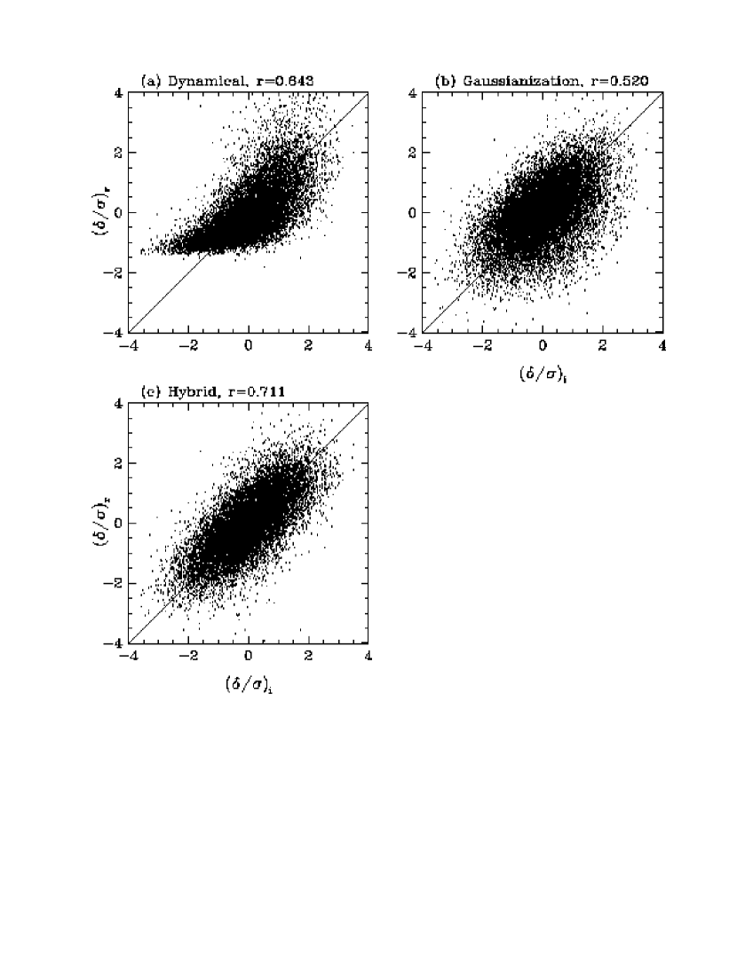
Figure 2: Cell by cell comparison of the reconstructed initial density contrast $({\delta}/{\sigma})_{r}$ to the true initial density contrast $({\delta}/{\sigma})_{i}$ for (a) dynamical reconstruction, (b) Gaussianization, and (c) the hybrid method. All the density fields are smoothed with a Gaussian filter of radius $R_{s}=3h^{-1}$Mpc and scaled by the rms fluctuation $\sigma$. The correlation coefficient $r$ is indicated above each panel.

Figure 3 shows the power spectrum of the true initial density field (dotted line), the reconstructed initial conditions (solid line), and the reconstructed initial conditions prior to power restoration (dashed line, with arbitrary normalization). The dashed line displays the suppression of small scale power due to non-linear evolution, but this is corrected adequately by the power restoration step, as the good agreement in shape of the solid and dotted lines demonstrates. The power spectrum of the full hybrid reconstruction has a slightly lower amplitude than the true initial power spectrum (about $10\%$ lower amplitude in the power spectrum corresponding to about a $5\%$ lower amplitude for $\sigma_{8m}$). This may reflect the presence of residual non-Gaussianity in the reconstructed field, which we detected as a slight “meatball” shift in the genus curve (Melott, Weinberg, & Gott (1988)). Thus, although the 1-point probability distribution is Gaussian by construction, the N-point distributions of the recovered initial density field may be non-Gaussian. However, any impact of residual non-Gaussianity on the derived $P(k)$ normalization is quite weak, as shown by the good agreement between the true and the reconstructed power spectra in Figure 3.

Figure 3: Power spectrum of the true initial density field (dotted line), the density field reconstructed by steps (H1)-(H4) of the hybrid method (dashed line), and the hybrid reconstructed density field after the power restoration and amplitude matching procedures (solid line). The dashed line has been multiplied by the factor $e^{k^{2}R_{s}^{2}}$ in the range $0<k\leq k_{\rm corr}$ to restore the power lost in the Gaussian smoothing, and its amplitude has been fixed arbitrarily.

Figure 4 shows the true and the reconstructed final galaxy distributions. We plot the locations of the “galaxy” particles, a random subset of all the N-body particles, that lie in a region $40h^{-1}$Mpc thick about the center of the cube and extend in the $x$-$y$ plane from $(50,50)h^{-1}$Mpc to $(150,150)h^{-1}$Mpc. Comparing the locations of clusters in the three galaxy distributions, we see that the hybrid scheme (panel b) in general, recovers more accurate positions for the clusters than does Gaussianization alone (panel c). This improvement is clear, for example, in the corresponding locations of the clusters located near $(x,y)=(115,145)h^{-1}$Mpc and $(110,135)h^{-1}$Mpc in the true final galaxy distribution (panel a). There is also a cluster at $(x,y)=(80,50)h^{-1}$Mpc in the Gaussianization reconstruction. This cluster is located in an adjacent slice in the true and hybrid reconstructed galaxy distributions. We will quantify the agreement in the cluster locations below. Panel (d) shows the final galaxy distribution reconstructed by the hybrid scheme assuming (incorrectly) that the galaxy distribution is biased with $b=2$. We explain the biasing scheme that we used to get this galaxy distribution in §3.2. This biased galaxy distribution clearly appears more diffuse compared to the true galaxy distribution. We will quantify this diffuse appearance using the nearest neighbor statistic described below.

Figure 4: Final galaxy distributions, with $\sigma_{8g}=1.1$. The panels show galaxy distributions in a slice $40h^{-1}$Mpc thick and spanning $100h^{-1}$Mpc in the other two dimensions. (a) True final galaxy distribution (unbiased). (b) Hybrid reconstruction assuming unbiased galaxy formation. (c) Gaussianization assuming unbiased galaxy formation. (d) Hybrid reconstruction assuming biased galaxy formation with $b=2$.

Figure 5 shows a scatter plot of the final density fields after smoothing with a Gaussian filter of radius $R_{s}=3h^{-1}$Mpc and scaling by the rms fluctuation. The correlation is much stronger for the hybrid reconstruction (panel a) compared to Gaussianization alone (panel b), as would be expected from the greater dynamical accuracy of the hybrid method.

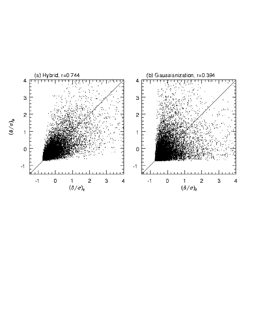
Figure 5: Cell by cell comparison of the reconstructed final density contrast $(\delta/\sigma)_{r}$ to the true final density contrast $(\delta/\sigma)_{f}$ for (a) Hybrid reconstruction and (b) Gaussianization. The density fields are smoothed with a 3$h^{-1}$Mpc Gaussian filter and scaled by the rms fluctuation $\sigma$. The linear correlation coefficient $r$ is indicated above each panel.

Clusters are the most massive collapsed structures in the final galaxy distributions. The abundance and masses of clusters encode important information regarding the amplitude of mass fluctuations and the value of $\Omega$ (White, Efstathiou, & Frenk (1993); Eke, Cole, & Frenk (1996); Cole et al. (1997); Fan, Bahcall, & Cen (1997)). Therefore, we analyze the extent to which the locations and properties of clusters can be reproduced by the different reconstruction procedures. We identify the clusters in the galaxy distributions using the standard friends of friends algorithm (Davis et al. (1985)), with a linking length parameter $b=0.2\bar{d}$, where $\bar{d}=4.64h^{-1}$Mpc is the mean inter-galaxy separation. The mean overdensity of clusters selected with this linking parameter is approximately 250, corresponding roughly to the criterion for virial equilibrium. We also require that a cluster contain at least 10 galaxies.

We match the clusters in the true and the reconstructed galaxy distributions using the algorithm described by Weinberg, Hernquist & Katz (1997). We first sort the cluster lists in descending order of cluster masses. Then, for every cluster in the true final galaxy distribution, we find the most massive unmatched cluster in the reconstructed galaxy distribution whose centroid lies within a distance $l=12h^{-1}$Mpc from the centroid of the original cluster. We repeat this procedure for progressively less massive clusters until we complete the cluster list of the true galaxy distribution. The results that we show below are not sensitive to reasonable variations in the values of $l$, although for a shorter matching length a larger fraction of clusters remains unmatched in the end. The histograms in Figure 6 show the number of clusters that match between the true and the reconstructed final galaxy distributions as a function of the distance between their centroids. The solid and the dashed lines show this statistic for the hybrid and Gaussianization reconstruction schemes, respectively. The dotted line shows the number of clusters that can match randomly between the true and the hybrid reconstructed galaxy distributions. We estimate this by interchanging the $x$ and $y$ coordinates of the clusters in the hybrid reconstruction and matching the clusters using the same algorithm. Comparison of the solid and dashed histograms demonstrates the clear superiority of the hybrid reconstruction method: while the total number of matched clusters is similar for the two reconstructions (about 400), the hybrid scheme puts clusters closer to their actual locations. This is precisely the sort of improvement we expect from the greater dynamical accuracy of the hybrid method.

Figure 6: Cluster matching statistics for the final galaxy distributions of the hybrid reconstruction scheme (solid line) and Gaussianization (dashed line). Clusters in the true final galaxy distribution are matched to the most massive unmatched cluster in the reconstructed galaxy distribution within a radius of $12h^{-1}$Mpc. The dotted line shows the expected number of random matches; it is obtained by interchanging the $x$ and $y$ coordinates of clusters in the hybrid reconstruction and then matching.

In Figure 7, we compare the multiplicities of the matched clusters in the true and the reconstructed galaxy distributions. Circles show the multiplicities of clusters that are matched between the true and the reconstructed galaxy distributions. Crosses parallel to either axis represent clusters that are present in one galaxy distribution (true/reconstructed), but not matched to a corresponding cluster in the other (reconstructed/true) galaxy distribution. The scatter for the massive clusters (log $N_{c}>1.5$) is much smaller for the hybrid scheme (panel a) than for the Gaussianization reconstruction (panel b). The hybrid scheme also matches a larger fraction of these clusters, as shown by the smaller number of crosses along either axis at $\log N_{c}>1.5$.

Figure 7: Comparison of the cluster multiplicities between the true final galaxy distribution and the reconstructed galaxy distribution for (a) the hybrid reconstruction scheme and (b) Gaussianization. Crosses parallel to either axis represent clusters present in that galaxy distribution alone.

Thus far, we have directly compared the recovered initial density fields and the reconstructed final galaxy distributions for the various reconstruction methods with the true initial density field and the true final galaxy distribution. These comparisons have helped us understand the accuracy of the reconstruction methods and have shown that the hybrid method is superior to the Gaussianization and dynamical methods in its ability to reproduce the observed features. We now compare the global statistical properties of the input and reconstructed galaxy distributions. Since the hybrid reconstruction has a significantly higher dynamical accuracy than the Gaussianization method, we show the results of our statistical comparisons for the hybrid reconstruction only.

The main purpose of the global statistical comparisons is to test the effects of the different assumptions that enter the reconstruction procedure. In this section we focus on the bias factor, and we therefore compare the results of an unbiased hybrid reconstruction of an unbiased true galaxy distribution (the model) to the results of the hybrid reconstructions of the same model that assume (incorrectly) that the galaxy distribution is biased with bias factors of $b=2$ or $b=3$. We perform the hybrid reconstructions of the input model by following the procedures described in §2. The specific biasing scheme that we use in step (H6B) is described in §3.2 below. We show the galaxy distribution that is reconstructed by the hybrid method assuming $b=2$ in Figure 4d. We have applied numerous statistical measures to the input and the reconstructed galaxy distributions, although we show only two of these here: the two-point correlation function $\xi(r)$ and the nearest neighbor distribution $P(x_{n})$. When we analyze the mock catalogs of redshift surveys in §4, we will also examine the angular anisotropy of the redshift space correlation function $\xi(s,\mu)$, which is induced by the peculiar velocities of galaxies.

Figure 8 shows the two-point correlation function $\xi(r)$ for the true unbiased galaxy distribution (dotted line) and for the hybrid reconstructed galaxy distributions with different assumptions about bias. We see that the $\xi(r)$ of the hybrid reconstruction assuming (correctly) unbiased galaxy formation matches the true $\xi(r)$ very well on all scales (solid line). However, hybrid reconstruction assuming (incorrectly) $b=3$ leads to a shallower $\xi(r)$, with a weak clustering strength on small scales (dot-dashed line). For an observed value of $\sigma_{8g}$, the amplitude of mass fluctuations is a decreasing function of $b$. Therefore, the mass distribution in an unbiased scenario is more dynamically evolved and has a steeper $\xi(r)$ than in the corresponding biased case. Biasing can amplify the mass clustering to match the input $\xi(r)$ on large scales, but it cannot simultaneously achieve the strong small scale clustering that is produced by gravitational collapse. The deficit of small scale clustering is not seen clearly in $\xi(r)$ for the $b=2$ hybrid reconstruction (dashed line), presumably because the effect of biasing is not strong enough compared to the effects of gravitational evolution at this level of bias.

Figure 8: $\xi(r)$ for the final galaxy distributions: true final galaxy distribution assuming unbiased galaxy formation (dotted line), hybrid reconstruction assuming unbiased galaxy formation (solid line), and hybrid reconstructions assuming biased galaxy formation with $b=2$ (dashed line) and $b=3$ (dot-dashed line).

In Figure 9, we plot the distribution of distances to the nearest neighbor of each galaxy $P(x_{n})$ for the true unbiased galaxy distribution (dotted line) and for the reconstructions with different assumptions regarding bias. To remove its dependence on the average density of galaxies, this distribution is expressed in terms of $x_{n}$, which is equal to the separation $r_{n}$ divided by the mean inter-galaxy separation $\bar{d}\equiv n_{g}^{-1/3}$ (i.e, $x_{n}=r_{n}/\bar{d}$). At separations smaller than the force resolution of our PM code, the exact behavior of this distribution cannot be estimated reliably. Therefore, we show only the mean level of the distribution for $x_{n}<0.2$, corresponding roughly to distances $r_{n}<1h^{-1}$ Mpc. We normalize the distributions in Figure 9 so that

$$\int_{0}^{\infty}P(x_{n})dx_{n}=1.$$ (12)

We see that the reconstruction that correctly assumes an unbiased galaxy distribution (solid line) reproduces the true $P(x_{n})$ (dotted line) very well. The biased reconstructions have undergone weaker non-linear evolution, and they therefore have fewer galaxy pairs at close separations and correspondingly more pairs at $x_{n}\sim 0.4$. This statistic clearly captures and quantifies the diffuse appearance of the $b=2$ reconstruction that is shown in Fig. 4d. The effects of gravitational evolution are still weaker in the hybrid reconstruction with $b=3$, and the corresponding $P(x_{n})$ (dot-dashed line) is much flatter than that of the true unbiased galaxy distribution.

Figure 9: Nearest neighbor distribution for the final galaxy distributions in terms of $x_{n}$, the separation $r_{n}$ divided by the mean inter-galaxy separation $\bar{d}$. Dotted, solid, dashed, and dot-dashed lines show, respectively, the true, unbiased final galaxy distribution, the hybrid reconstruction assuming unbiased galaxy formation, and hybrid reconstructions assuming biased galaxy formation with $b=2$ and $b=3$.

Based on the tests in this section, we can arrive at the following two conclusions regarding the performance and the use of the hybrid reconstruction method.

(1)

The hybrid reconstruction method performs significantly better than either the dynamical scheme or the Gaussianization method in reconstructing unbiased, real space galaxy distributions. We also carried out the relevant comparisons while reconstructing biased galaxy distributions and mock redshift catalogs and always found that the hybrid method yields the most accurate reconstruction. Therefore, in subsequent sections, we will only show the results of the hybrid reconstruction.

(2)

Biased reconstructions of unbiased models produce insufficient small scale clustering for a given level of fluctuations in the final galaxy distribution ($\sigma_{8g}$). We are able to detect this failure visually and by using statistical measures like the nearest neighbor distribution. We conclude that reconstruction analysis can be used to test the hypothesis of biased galaxy formation.

3.2 Biased Reconstructions

We now test the ability of the hybrid scheme to reconstruct biased galaxy distributions and further test its ability to detect incorrect assumptions about bias. We perform all the simulations using the same parameters as in the unbiased case except for the amplitude of the initial fluctuations. We normalize the amplitude of the initial power spectrum so that $\sigma_{8m}=\sigma_{8g}/b=0.55$ for a bias factor $b=2$. We evolve this initial density field through a PM code and select “galaxies” from this evolved mass distribution using a local power law biasing relation between the mass density $\rho_{m}$ and the galaxy density $\rho_{g}$ (Mann, Peacock, & Heavens (1998)):

$$\log\left(\frac{\rho_{g}}{\langle\rho_{g}\rangle}\right)=A+B\log\left(\frac{\rho_{m}}{\langle\rho_{m}\rangle}\right).$$ (13)

We choose the constants $A$ and $B$ so that the resulting galaxy distribution has the desired average number density $n_{g}=0.01h^{3}$Mpc^-3 and rms fluctuation amplitude $\sigma_{8g}=1.1$. The probability that a mass particle in a region where the mass density is $\rho_{m}$ is chosen as a galaxy is proportional to $\rho_{m}^{B-1}$. We compute the mass density $\rho_{m}$ in a sphere of radius $5h^{-1}$Mpc around the particle. This biasing relation is similar to the one suggested by Cen & Ostriker (1993) based on hydrodynamic simulations incorporating physical models for galaxy formation (Cen & Ostriker (1992)), but it differs in that there is no quadratic term that saturates the biasing relation at high values of the mass density.

In all the tests of reconstructions of biased galaxy distributions, we adopt as the true galaxy distribution (the input data) a fiducial galaxy distribution with $\sigma_{8g}=1.1$, biased to $b=2$ using the prescription defined by equation (13). We compare this true distribution to a biased hybrid reconstruction that correctly assumes $b=2$. We will also show some comparisons to reconstructions that incorrectly assume unbiased galaxy formation or biased galaxy formation with $b=3$. When biasing the evolved mass distributions in step (H6B), we use the same power-law biasing prescription that we adopted for the true model.

Figure 10 shows the contour plots of the true initial density field and the hybrid reconstructed density field assuming (correctly) $b=2$. The contours are plotted in the same slice as in Figure 1. Comparing Figure 10 to Figure 1, we see that the recovery of the initial conditions is more accurate in the biased model, because the effect of non-linear gravitational evolution is smaller in the biased case. Figure 11a shows a scatter plot of the true and reconstructed initial density contrasts. Comparison to Figure 2c again shows the more accurate recovery of initial densities in the biased model, quantified by the increase in the correlation coefficient from $r=0.711$ to $r=0.813$. The more accurate initial conditions yield a more accurate final galaxy density field, as shown by comparing the final density scatterplot (Fig. 11b) to the corresponding plot for the unbiased model (Fig. 5a).

Figure 10: Contours in a slice of the initial density field of a test N-body simulation. The contour levels range from $-2\sigma$ to $+2\sigma$ in steps of $0.4\sigma$. Solid contours correspond to overdensities, while dashed contours correspond to underdensities. (a) True initial conditions, Gaussian with a $\Gamma=0.25$ power spectrum. A slice through the galaxy distribution obtained by gravitationally evolving this field and then selecting galaxies with $b=2$ is shown in Fig. 12a. (b) The initial density field reconstructed from this biased galaxy distribution assuming $b=2$.

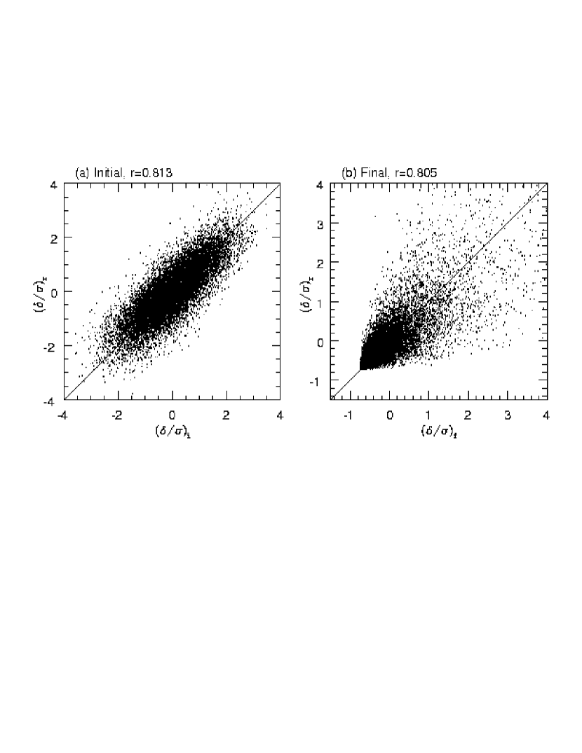
Figure 11: (a) Cell by cell comparison of the reconstructed initial density contrast $(\frac{\delta}{\sigma})_{r}$ and the true initial density contrast $(\frac{\delta}{\sigma})_{i}$ for the hybrid reconstruction of the biased model. (b) Comparison of the true and reconstructed final density contrasts. All the density fields are smoothed with a Gaussian filter of radius $R_{s}=3h^{-1}$Mpc and scaled by the rms fluctuation $\sigma$. The linear correlation coefficient $r$ is indicated above each panel.

Figure 12 shows the power spectrum of the true initial density field by a dotted line. The power spectrum of the density field reconstructed using the steps (H1), (H2B), (H3) and (H4) of the hybrid method (i.e., with no power restoration) is shown by the dashed line. The solid line shows the power spectrum after the power restoration and the amplitude matching procedures. By construction, the amplitude of the power spectrum is normalized so that $\sigma_{8m}=\sigma_{8g}/b=0.55$ for the assumed value of $b=2$. The wavenumber beyond which random phase waves are added ($k_{\rm corr}=20k_{f}=0.628\ h$Mpc^-1) is marked in the Figure.

Figure 12: Power spectrum of the true initial density field (dotted line), the density field reconstructed using steps (H1), (H2B), (H3) and (H4) of the hybrid method (dashed line), and the hybrid reconstructed density field after the power restoration and amplitude matching procedures (solid line). The final galaxy distribution is biased with $b=2$. The dashed line has been multiplied by the factor $e^{k^{2}R_{s}^{2}}$ in the range $0<k\leq k_{\rm corr}$ to restore the power lost in the Gaussian smoothing, and its amplitude has been fixed arbitrarily.

Figure 13a shows the true final galaxy distribution when the galaxies are biased tracers of the mass distribution with a bias factor $b=2$. This galaxy distribution is noticeably more diffuse than the unbiased galaxy distribution shown in Figure 4a, although the rms fluctuation amplitude $\sigma_{8g}$ is identical for both distributions. The galaxy distribution reconstructed by the hybrid scheme, assuming biased galaxy formation with a correct value of $b=2$, is shown in Figure 13b. The individual structures and the overall texture of the galaxy distribution appear very similar to those of the true distribution. The statistical properties of this galaxy distribution closely match those of the true distribution, as shown below. The reconstructed galaxy distribution assuming unbiased galaxy formation (Fig. 13c) shows clear evidence for excessive dynamical evolution. Clusters are more prominent and larger structures more clumpy than in the true galaxy distribution. The reconstruction assuming $b=3$ (Fig. 13d) does not have enough non-linear structure and appears very diffuse. This diffuse appearance can be easily quantified by the nearest neighbor statistic, as we will show below.

Figure 13: Final galaxy distributions, with $\sigma_{8g}=1.1$ (a) True final galaxy distribution in the model with biased galaxy formation with $b=2$. Remaining panels show hybrid reconstructions assuming (b) biased galaxy formation with $b=2$, (c) unbiased galaxy formation and (d) biased galaxy formation with $b=3$.

Figure 14 shows the two-point correlation functions $\xi(r)$ of the true galaxy distribution and the galaxy distributions reconstructed with different assumptions about biasing. The reconstruction with $b=2$ matches the true $\xi(r)$ closely on all scales. Unbiased reconstruction leads to excessive clustering on small scales, resulting in a correlation function that is steeper than that of the input data. The final galaxy distribution in the $b=3$ reconstruction is less dynamically evolved and has a shallow $\xi(r)$ on small scales.

Figure 14: Correlation functions $\xi(r)$ for the true final galaxy distribution of the biased model (dotted line) and for the hybrid reconstructions assuming biased galaxy formation with $b=2$ (solid line), biased galaxy formation with $b=3$ (dot-dashed line), and unbiased galaxy formation (dashed line).

The dotted line in Figure 15 shows the nearest neighbor distribution of the true galaxy distribution. The solid line that closely matches this dotted line corresponds to the hybrid reconstruction with the correct assumption for the bias factor $b=2$. The excessive small scale clustering in the unbiased reconstruction produces a steeper distribution (dashed line), while the $b=3$ reconstruction has a flatter nearest neighbor distribution (dot-dashed line) that reflects its smaller degree of non-linear evolution. This statistic quantifies well the appearance of the galaxy distributions in Figure 13, and it can therefore serve as a discriminatory statistic to distinguish between different assumptions about bias.

Figure 15: Nearest neighbor distribution for the final galaxy distributions, with the same coding as in Fig. 14.

The tests in this section show that the hybrid reconstruction scheme can be applied successfully to biased galaxy distributions. Once again, we get the best recovery of the initial density fields and the final galaxy distributions if we make the correct assumptions about the bias between the final mass and galaxy distributions. Incorrect assumptions lead to galaxy distributions that are incompatible with the input data, and this incompatibility can be quantified by the nearest neighbor distribution and the two-point correlation function, though the latter is only marginally effective in distinguishing among reconstructions with modest differences in the bias factor. We also find that, for a given level of $\sigma_{8g}$, the effects of bias are more easily reversed than the effects of non-linear gravitational evolution.

4 TESTS ON ARTIFICIAL REDSHIFT SURVEY CATALOGS

The primary requirements for a redshift survey to be suitable for reconstruction analysis are good sky coverage and depth so that the gravitational influence of regions outside the survey boundaries is small, dense sampling to reduce shot noise errors, and a well understood selection function. Of existing redshift surveys, the IRAS-selected, Point Source Catalog Redshift Survey (PSCZ, see Saunders et al. (1995) and Canavezes et al. (1998)) best satisfies the above requirements. However, IRAS and optically selected galaxies are known to cluster differently (e.g., Lahav, Nemiroff, & Piran (1990); Saunders, Rowan-Robinson, & Lawrence (1992); Fisher et al. (1994)), so it is also desirable to analyze an optically selected galaxy distribution using the reconstruction procedure, partly in order to understand the origin of this clustering difference. Of course, the optical and the IRAS galaxies in a given region are both related to the same underlying mass distribution. The Optical Redshift Survey (ORS, Santiago et al. 1995, 1996) is probably the best existing optical survey for reconstruction analysis because of its nearly full sky coverage, even though there are other surveys that contain more galaxies. We hope to analyze both the PSCZ and the ORS using the hybrid reconstruction procedure in the near future. Here, we analyze artificial redshift catalogs that are designed to mimic these surveys, in order to test the ability of the reconstruction method to handle redshift space input data with non-periodic survey boundaries and to see what we can expect to learn from the reconstruction analysis of these catalogs.

We construct the mock redshift catalogs from the output of a PM simulation of an $\Omega=0.4$ universe, assuming Gaussian initial fluctuations with a $\Gamma=0.25$ power spectrum. This simulation evolves $100^{3}$ particles in a periodic cube of side $200h^{-1}$Mpc and uses a $200^{3}$ mesh to compute the gravitational forces. We assume that the galaxies in the mock PSCZ catalog form in an unbiased manner with $\sigma_{8g}=\sigma_{8m}=0.75$, while the ORS galaxies are biased tracers of the same mass distribution with $\sigma_{8g}=1.1$. We reconstruct the galaxy distributions of these two mock catalogs using the hybrid reconstruction scheme. In the power restoration step, we correct the power spectrum using empirical correction factors for $k_{f}\leq k\leq k_{\rm corr}=15k_{f}=0.471\ h$Mpc^-1, and we add random phase waves for higher wavenumbers in the manner described in §2. We normalize the power spectrum by requiring that the final $\sigma_{8g}$ of the reconstructed galaxy distribution match that of the mock catalog in redshift space. While in the previous section we showed how the degree of clustering on small and large scales can be used to constrain the bias factor, here we will focus mainly on our ability to constrain $\Omega$, given the correct assumptions about the bias factor. Therefore, we will reconstruct the two mock redshift catalogs assuming both $\Omega=0.4$ (the correct value) and $\Omega=1$. Any systematic failure of the $\Omega=1$ reconstruction to reproduce the input data will tell us about the discriminatory power of the reconstruction method. We do, however, expect some tradeoff between $\Omega$ and $b$, if both parameters are allowed to vary simultaneously.

We select a Local Group observer from the final particle distribution so that the velocity dispersion in a sphere of radius $5h^{-1}$Mpc around that observer is less than $250$ km s^-1, in accord with observations that imply a cold velocity field near the Local Group (Sandage (1986); Brown & Peebles (1987)). We assign each galaxy a redshift based on its real space distance and its radial peculiar velocity with respect to this Local Group particle. We use the same Local Group observer for both the mock catalogs so that the underlying mass distribution is identical in the regions where the two surveys overlap. To create the mock redshift catalogs, we first select volume limited subsamples of the galaxy distribution extending to an inner radius $r_{\rm in}$. We supplement this volume limited sample with an extended magnitude limited sample out to a larger radius $r_{\rm out}$, so as to improve the reconstruction near the boundaries of the inner sample. We reject all the galaxies in an angular mask about the observer to account for the incompleteness of the surveys in the regions corresponding to the Galactic zone of avoidance (ZOA).

We form the final galaxy density fields by CIC binning the galaxies in the mock redshift catalogs onto a $100^{3}$ cubical grid that represents a region $200h^{-1}$Mpc a side. In the region $r<r_{\rm in}$, we assign equal weights to all the galaxies, as the catalog is volume limited up to that radius. In the region $r_{\rm in}<r<r_{\rm out}$, we weight each galaxy by the inverse of the value of the selection function $\phi(r)$ at its location. In the regions outside the survey boundaries, we set the density field to be equal to its mean value inside the survey region. We account for boundary effects in computing the smoothed density field $\rho_{sm}({\bf r})$ by using the ratio method of Melott & Dominik (1993),

$$\rho_{sm}({\bf r})=\frac{\int M({\bf r^{\prime}})\rho({\bf r^{\prime}})W({\bf r-r^{\prime}})d^{3}{\bf r^{\prime}}}{\int M({\bf r^{\prime}})W({\bf r-r^{\prime}})d^{3}{\bf r^{\prime}}},$$ (14)

where $W({\bf r})$ is the smoothing filter and the mask array $M({\bf r})$ is set to 1 for pixels inside the survey region and to 0 for pixels outside the survey region.

4.1 Correction for Redshift Space Distortions

Redshifts of galaxies reflect the combination of Hubble flow at their real space locations and the radial component of the peculiar velocities acquired during gravitational evolution. This peculiar velocity component distorts the mapping of galaxy positions from real to redshift space, making the line of sight a preferred direction in an otherwise isotropic universe. However, we need the mass density field in real space in order to recover the initial mass density fields using the hybrid reconstruction method. Therefore, we need to correct for these peculiar velocity induced distortions. The effects of these distortions on the redshift space density field are different on different scales.

On small scales, the velocity dispersion associated with a cluster stretches it along the line of sight into a “Finger of God” feature that points directly toward the observer. This feature spreads a compact cluster in real space over a large radial distance in redshift space and thus reduces the amplitude of small scale clustering. To correct for this effect, we first identify the clusters in redshift space using a friends-of-friends algorithm that employs different linking lengths in the radial and transverse directions (Huchra & Geller (1982); Nolthenius & White (1987); Moore, Frenk, & White (1993)). Here we use a transverse linking length of $0.6h^{-1}$Mpc and a radial linking length of $500$ kms^-1 (Gramann, Cen, & Gott (1994)). For each cluster, we shift the radial locations of the member galaxies so that the resulting compressed cluster has a radial velocity dispersion of $100$ kms^-1, roughly the value expected from Hubble flow across its physical extent.

The distortions on large scales arise from coherent inflows into overdense regions and outflows from underdense regions (Sargent & Turner (1977); Kaiser (1987)). These bulk flows are generated by large scale density fluctuations that can be reasonably assumed to be still in the quasi-linear regime of gravitational evolution. To remove these large scale distortions and estimate the real space mass density field, we apply a modified version of the iterative procedure suggested by Yahil et al. (1991) and Gramann, Cen & Gott (1994) to the cluster-compressed, redshift space galaxy distribution:

(R1):

For biased galaxy density fields, we first apply a monotonic local map to the redshift space galaxy density field that enforces a numerically determined PDF of the real space mass density field corresponding to the assumed value of the bias factor $b$. This mapping provides our zero-th order estimate of the real space mass density field, correcting for the effects of bias and peculiar velocity distortions on the PDF. We could apply a similar mapping even for the unbiased case, in the hope of having a more accurate starting point for peculiar velocity corrections. In practice, however, we find that this mapping does not significantly improve the convergence of the iterative procedure, so we ignore it in the unbiased reconstruction.

(R2):

We predict the velocity field from this mass density field using Gramann’s (1993b) second-order perturbation theory relation,

$${\bf v(r)}=f(\Omega)H\left[{\bf g(r)}+\frac{4}{7}\nabla C_{g}({\bf r})\right],$$ (15)

where ${\bf g(r)}$ is the gravitational acceleration field computed from the equation $\nabla\cdot{\bf g(r)}=-\delta({\bf r})$ and $C_{g}$ is defined by equation (6). This step requires that we assume a value of $\Omega$ to compute the factor $f(\Omega)$.

(R3):

We use this velocity field information to correct the positions of galaxies so that their new positions are consistent with their Hubble flow velocities and the peculiar velocities at their locations.

We iterate these three steps until the corrections to the galaxy locations in step (R3) become negligible and the galaxy density field has converged. In practice, we find that the positional corrections become very small in about three steps. We use the mass density field derived from the inferred real space galaxy distribution as the input to the hybrid reconstruction scheme. In the last step of the reconstruction, after selecting galaxies from the evolved N-body mass distribution in an unbiased or biased manner, we project these galaxies into redshift space, so that we can compare the reconstructed and the true input galaxy distributions directly in redshift space.

4.2 Reconstruction of a Mock PSCZ Catalog

The PSCZ survey contains all galaxies in the IRAS Point Source Catalog whose $60\mu m$ flux is greater than $0.6$Jy, excluding the regions that are heavily contaminated by Galactic sources (mainly the low Galactic latitude zone $|b|<5^{\circ}$). The catalog contains about $15,500$ galaxies and covers about $83\%$ of the sky. We create a mock catalog of this survey by selecting a volume limited sample from an unbiased galaxy distribution extending to $r_{\rm in}=55h^{-1}$Mpc at an average density of $0.01h^{3}$Mpc^-3. We also include a magnitude limited sample to $r_{\rm out}=75h^{-1}$Mpc, with the selection function decreasing as $\phi(r)\propto r^{-4}$ in the region $r_{\rm in}<r\leq r_{\rm out}$. We exclude all galaxies in a 10^∘ wedge to mimic the survey’s Galactic plane cut. We reconstruct the mock catalog assuming that the galaxy distribution is unbiased with respect to the mass distribution.

Figure 16 shows isodensity contours of the true and reconstructed initial density fields in a slice through the center of the mock PSCZ survey. The hybrid scheme recovers the true initial density field quite accurately in the inner regions, although near the boundaries the density field recovery is poor. The clumping of contours at the edges is an artifact of the graphing routine; the true and reconstructed density fields are actually continuous across the boundaries.

Figure 16: Contours in a slice of the initial density field for the mock PSCZ survey. The contour levels range from $-2\sigma$ to $+2\sigma$ in steps of $0.4\sigma$. Solid contours correspond to overdensities, while dashed contours correspond to underdensities. (a) True initial conditions from a $\Gamma=0.25$ power spectrum. A slice through the galaxy distribution evolved from this field and selected using the PSCZ survey geometry appears in Fig. 18a. (b) The initial density field recovered by the hybrid reconstruction method. The 10^∘ Galactic plane cut can be seen near $z=0$.

Figure 17a shows a scatter plot of the true and reconstructed initial density fields. The scatter is greater than that for the corresponding unbiased full cube reconstruction (Fig. 2c), even though the final galaxy density field is less non-linear here ($\sigma_{8g}=0.75$ for the mock PSCZ catalog, as opposed to 1.1 in the full cube simulations). This larger scatter probably reflects the gravitational influence of regions beyond the survey boundaries that cannot be accounted for due to the finite volume of the survey. Nevertheless, we see that it is possible to recover the initial density fields quite accurately from a realistic galaxy catalog. The comparison of the final density fields in Figure 17b shows that the hybrid scheme reproduces the true galaxy density field without any major systematic errors.

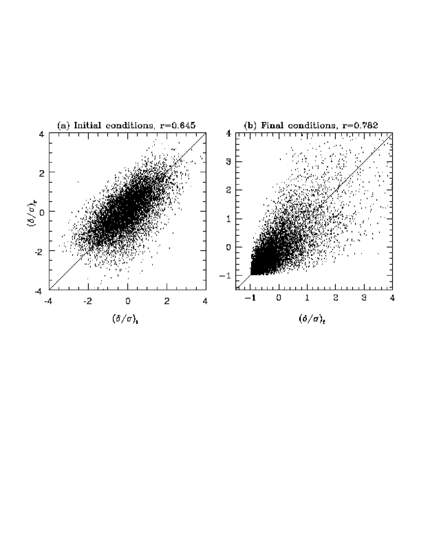
Figure 17: (a) Cell by cell comparison of the hybrid reconstructed initial density contrast $(\delta/\sigma)_{r}$ to the true initial density contrast $(\delta/\sigma)_{i}$ for the mock PSCZ catalog. (b) Comparison of the reconstructed final density contrast $(\delta/\sigma)_{r}$ to the true final density contrast $(\delta/\sigma)_{f}$, in redshift space. All the density fields are smoothed with a Gaussian filter of radius 3$h^{-1}$Mpc and scaled by the rms fluctuation $\sigma$. The linear correlation coefficient $r$ is indicated above each panel.

Figure 18 shows the power spectra of the true initial density field (dotted line) and the hybrid reconstructed density fields after the power restoration and amplitude normalization procedures. The solid and the dashed lines show the reconstructed power spectrum assuming $\Omega=0.4$ (the correct value) and $\Omega=1$ respectively. The slight amplitude mismatch arises from the residual errors present in the recovered initial density field.

Figure 18: Power spectrum of the true initial density field of the mock PSCZ survey (dotted line) and the normalized, hybrid reconstructed density field recovered for $\Omega=0.4$ (the correct value, solid line) and for $\Omega=1$ (incorrect value, dashed line). The arrows show the wavenumber that corresponds to the survey size ($k_{\rm surv}=2\pi/2r_{\rm in}=0.0571\ h$Mpc^-1) and the wavenumber $k_{\rm corr}=15k_{f}=0.471\ h$Mpc^-1 beyond which random phase waves are added to the reconstructed field.

Figure 19 shows the true and the reconstructed galaxy distributions of the mock PSCZ survey in real space (top panels) and redshift space (bottom panels). All the galaxies in a $40h^{-1}$Mpc thick slice centered on the Local Group are shown. Comparing panels (a) and (b), we see that the prominent clusters are reproduced at the appropriate locations. However, a notable failure is the absence in the reconstructed galaxy distribution of the filamentary structure that runs from $(x,z)=(-5,20)h^{-1}$Mpc to $(5,40)h^{-1}$Mpc in the mock PSCZ survey. This structure was not present in the adjacent slices either. We did, however, find an extra cluster at that location in the slice that lies above the one shown in the Figure. We found that this filamentary structure is actually comprised of clusters that appear close together in projection. One of the clusters that is closest to the top edge of the slice has moved to an adjacent slice during reconstruction, thereby destroying the apparent “filament”.

Figure 19: Final galaxy distributions for the mock PSCZ catalog reconstruction in the region $-20<y<20h^{-1}$ Mpc. (a) True final galaxy distribution in real space. (b) Final galaxy distribution of the hybrid reconstruction in real space. (c) True final galaxy distribution in redshift space. (d) Final galaxy distribution of the hybrid reconstruction in redshift space.

Figures 20a and 20b compare the cluster multiplicities and cluster velocity dispersions between the true and the reconstructed mock PSCZ catalogs. We identify the clusters in the redshift space galaxy distributions using the friends-of-friends algorithm described in §4.1. We match the clusters in the true and reconstructed redshift galaxy distributions using the algorithm explained in §3.1. The open symbols show the cluster comparison for a reconstruction assuming $\Omega=0.4$, while the filled symbols show the comparison for a reconstruction assuming $\Omega=1$. The squares parallel to either axis represent clusters present in that galaxy distribution alone.

A larger number of clusters are matched in the reconstruction that assumes the correct value of $\Omega=0.4$. The $\Omega=1$ reconstruction leaves several of the most massive clusters unmatched. Furthermore, the velocity dispersions of clusters in the $\Omega=1$ reconstruction are systematically higher than those in the true input galaxy distribution. This behavior is expected because the amplitude of fluctuations $\sigma_{8}$ is matched to that of the input galaxy distribution in both cases, and the average mass density is higher in an $\Omega=1$ universe. The clusters in an $\Omega=1$ reconstruction are therefore more massive and have a higher velocity dispersion. This comparison shows that the velocity dispersion of clusters in the reconstructed galaxy distribution can be used to constrain the value of $\Omega$, although the constraint will be weakened if the bias factor is not known a priori.

Figure 20: Comparison of (a) cluster multiplicities and (b) cluster velocity dispersions for the mock PSCZ catalog reconstructions. Values from the reconstruction are plotted on the $y$-axis against those from the true mock catalog galaxy distribution. Squares parallel to either axis represent clusters present in that galaxy distribution alone. Open symbols show the reconstruction with $\Omega=0.4$ (correct value), and filled symbols show a reconstruction with $\Omega=1$.

The peculiar velocities of galaxies affect the redshift space clustering on both small and large scales, as discussed in §4.1. The distortion caused by the velocity dispersions of collapsed clusters can be used to constrain $\Omega$ and $b$ as discussed above. We can also use the large scale, coherent flow distortions to constrain $\Omega$ and $b$. When the density fluctuations are small, the induced anisotropy of the redshift space correlation function $\xi(s,\mu)$ can be derived from linear perturbation theory (Kaiser (1987); Lilje & Efstathiou (1989); Hamilton 1993a ). This linear theory anisotropy depends solely on the parameter combination $\beta=\Omega^{0.6}/b$, which can therefore be inferred from the measured $\xi(s,\mu)$. A similar analysis can be performed using the redshift space power spectrum (Cole, Fisher, & Weinberg (1994)). However, these results are valid only when the density fluctuations are strictly in the linear regime, and this condition is generally violated on the scales accessible to existing redshift surveys. Attempts to estimate $\beta$ from redshift space distortions often assume a simple model for a position-independent, non-linear velocity component superposed on the linear flow (e.g., Fisher et al. (1994); Cole, Fisher, & Weinberg (1995)). The derived value of $\beta$ is only as good as the velocity model. Reconstruction, on the other hand, predicts the fully non-linear velocity field at the location of every galaxy. Thus, we can constrain the values of $\Omega$ and $b$ more accurately by demanding that a reconstruction reproduce the full angular anisotropy of the redshift space correlation function.

Figure 21 shows the correlation functions $\xi(s,\mu)$ for the mock PSCZ catalog and its $\Omega=1$ and $\Omega=0.4$ reconstructions, in five different angular bins. We compute the correlation functions using the estimator of Hamilton (1993b),

$$\xi(s,\mu)=\frac{N_{DD}N_{RR}}{N_{DR}^{2}}-1,$$ (16)

where $N_{DD},N_{DR}$ and $N_{RR}$ are the number of galaxy-galaxy, galaxy-random, and random-random pairs with a separation $s$ at an angle $\theta=\cos^{-1}(\mu)$ to the line of sight in redshift space. We use a random catalog that has the same geometry and selection function as the true galaxy distribution and contains about 50,000 points distributed randomly within the survey volume. We consider only those galaxy pairs that subtend an angle smaller than $\alpha_{max}=60^{\circ}$ at the observer so that the lines of sight to both the galaxies in the pair are approximately parallel. The filled circles show the real space correlation function $\xi(r)$. Since the real space correlation function is isotropic, we compute it using all the galaxy pairs in the sample that are separated by a distance $r$. We compress clusters before measuring $\xi(s,\mu)$ so that the Finger-of-God suppression is minimized and it is easier to detect the large scale amplification, which reaches its maximum value for separations along the line of sight ($\theta=0,\mu=1$). The enhancement is clearly seen in the panel corresponding to $\mu=0.9$, where the redshift space correlation functions lie above the real space correlation function in the range of separations $r<10h^{-1}$Mpc. As expected, this large scale enhancement, which depends on $\beta$, is larger for the $\Omega=1$ reconstruction than for the $\Omega=0.4$ reconstruction.

Figure 21: Correlation functions of the mock PSCZ catalog and its reconstructions after compressing the clusters. The galaxy pairs contributing to the different panels have different orientations relative to the line of sight, $\mu=\cos(\theta)$. The filled circles show the real space correlation function of the mock catalog and are the same in all panels. The dotted line shows the redshift space correlation function of the mock catalog. The solid line shows the redshift space correlation function for a hybrid reconstruction using $\Omega=0.4$ (the correct value), while the dashed line is for a reconstruction with $\Omega=1$.

Statistical uncertainties in measurements of redshift space distortions arise mainly from the finite volume of the redshift surveys themselves. “Cosmic variance” noise has more impact on $\xi(s,\mu)$ measurements than on $\xi(r)$ measurements because $\xi(s,\mu)$ is not averaged over angles. Each coherent sheet or filament in the redshift survey causes an enhanced signal in the angular bin that corresponds to its orientation. The anisotropy signals from these randomly oriented structures would average to zero in an infinite survey, but in a finite volume they mask the anisotropy caused by peculiar velocities and produce statistical uncertainty in $\beta$ estimates. Reconstruction overcomes the cosmic variance error in redshift space distortion studies because a reconstruction reproduces the physical structures in the survey volume with their correct orientations. The $\xi(s,\mu)$ for a reconstruction (or a real galaxy map) is not exactly isotropic even in the absence of peculiar velocities, but the differences in $\xi(s,\mu)$ for reconstructions with different values of $\Omega$ are due solely to the differences in peculiar velocities, not to changes in the physical orientations of coherent structures.

We demonstrate this point in Figure 22, which shows the statistic $(\xi_{s}-\bar{\xi})/\bar{\xi}$, the fractional difference between the ensemble mean redshift space correlation function ${\overline{\xi(s,\mu)}}$ and the redshift space correlation function $\xi(s,\mu)$ for the true and the reconstructed mock PSCZ catalogs. We compute the mean correlation function $\overline{\xi(s,\mu)}$ and the cosmic variance band (shaded region) from an ensemble of 20 independent mock PSCZ catalogs, and we plot this statistic only when $\overline{\xi(s,\mu)}>0.1$. The filled squares show the fractional difference for the true redshift space correlation function of the primary mock catalog, i.e., the departure from the mean $\overline{\xi(s,\mu)}$ in our single survey volume. The solid line and the dashed line show the same statistic for the reconstructed galaxy distribution assuming $\Omega=0.4$ and $\Omega=1$, respectively. The angular anisotropy of the galaxy distribution reconstructed with the correct assumption for $\Omega$ matches the true angular anisotropy well within the cosmic variance band. On the other hand, although the $\Omega=1$ reconstruction clearly produces excessive anisotropy, especially so for $\mu=0.9$, it could only be marginally rejected in straight statistical comparisons because of the large cosmic variance band. However, it is clearly inferior to the $\Omega=0.4$ reconstruction and can be rejected at a large confidence level using the reconstruction analysis, mainly because a reconstruction with the correct $\beta$ can match the observed angular anisotropies to much better than the cosmic variance limit.

Figure 22: Fractional difference between the correlation function of the reconstruction and the mean correlation function in redshift space for a mock PSCZ catalog. The mean correlation function $\bar{\xi}$ and the $1\sigma$ cosmic variance band (shaded region) are computed from an ensemble of 20 independent mock PSCZ catalogs. The filled squares show the redshift space correlation for the mock catalog. The solid and dashed lines show the redshift space correlation function for hybrid reconstructions assuming $\Omega=0.4$ and $\Omega=1$ respectively.

Figure 23 shows the distribution of nearest neighbors in the mock PSCZ catalog and its reconstructions. If computed using the redshift space galaxy distribution, this statistic would show a spurious peak at distances corresponding to the velocity dispersions of typical galaxy groups. However, we would like to use this statistic to measure the degree of small scale clustering in the same manner as in the tests on full cube, real space galaxy distributions, Therefore, we estimate the nearest neighbor distribution from the redshift space galaxy distributions using the method suggested by Weinberg & Cole (1992). For every galaxy at a redshift $z$, we consider all the galaxies that lie within a redshift range $\Delta v<1000\ {\rm kms^{-1}}$ to be its potential nearest neighbor. Of these candidate neighbors, we then choose the galaxy that lies closest to this galaxy in the transverse direction, and we compute the distribution of this transverse separation $R_{t}$ divided by the mean inter-particle separation $\bar{d}$ (i.e, $x_{n}=R_{t}/\bar{d}$). The dotted line shows this distribution for the mock PSCZ catalog, while the solid and dashed lines show this statistic for the galaxy distributions that are reconstructed assuming $\Omega=0.4$ and $\Omega=1$ respectively. Both the reconstructions recover the nearest neighbor distribution of the input data quite accurately.

Figure 23: Nearest neighbor distribution for the final galaxy distributions of the mock PSCZ catalog and its reconstructions. The nearest neighbor distribution is computed in redshift space using tangential separations with a $\Delta v=1000\ {\rm kms^{-1}}$ line of sight cut. The dotted line shows the nearest neighbor distribution of the true final galaxy distribution in the mock PSCZ catalog. Nearest neighbor distributions of the hybrid reconstructions are shown for $\Omega=0.4$ (solid line) and $\Omega=1$ (dashed line).

The redshift space correlation function and the nearest neighbor distribution use the data from the redshift catalogs alone. We can constrain the cosmological parameters more effectively if we also have the data about the peculiar velocities of galaxies. Comparison between predicted and observed peculiar velocity fields is one of the main motivations for all-sky redshift surveys like PSCZ and ORS. The predictions often use the linear theory relation between the density and velocity fields and thus break down in non-linear regions characterized by multi-stream flows. Attempts to correct for this breakdown either use quasi-linear approximations between the density and velocity fields or assume that the true peculiar velocity field is a combination of the linear theory predicted field and a position-independent, random velocity dispersion. The power of these comparisons is then limited by the validity of the model for the non-linear components of the peculiar velocity field. Reconstruction, on the other hand, predicts the fully non-linear peculiar velocity field at each point in redshift space, thereby giving a velocity field that can be directly compared to peculiar velocity data without the need for any additional modeling or approximations. We now compare the velocity field reconstructed with different assumptions about $\Omega$ to see the accuracy to which we can reproduce the fully non-linear, true final velocity field.

Figure 24 shows the $x$ and $z$ components of the velocity field of the mock PSCZ survey and its reconstructions. This plot shows the velocity field in the same slice whose density field is plotted in Figure 16. We compute the velocity and the velocity dispersion at any point as the mean and the $1\sigma$ dispersion about this mean of the velocities of all the galaxies located within $5h^{-1}$Mpc of this point. Panel (a) shows the true velocity field of the mock PSCZ catalog. Panel (b) shows the velocity field of the reconstructed galaxy distribution assuming (correctly) $\Omega=0.4$. Panel (d) shows the same field for the $\Omega=1$ reconstruction. We also plot, in panel (c), the velocity field predicted from the galaxy density field by the linear theory relation, for $\Omega=0.4$. Although the linear theory reproduces the true velocity field quite accurately in the low density regions, it systematically overestimates it in the high density regions as it does not account for the deviation of the velocity vector from the gravitational vector during the evolution of overdense regions (Gramann 1993b ). The reconstruction assuming $\Omega=1$, on the other hand, systematically overestimates all the velocities, and the reconstructed velocity field is everywhere too hot compared to the true velocity field. The reconstruction with the correct assumption of $\Omega=0.4$ provides the best recovery of the true velocity field. The amplitude of the velocities is comparable to the true values, and the non-linear component in high density regions is recovered quite well.

Figure 24: Velocity fields of the true and reconstructed galaxy distributions for the mock PSCZ survey, averaged over a $5h^{-1}$Mpc top hat window. Only the $x$ and $z$ components of the velocity field in a slice through the center of the survey are shown. (a) Velocity field of the true mock PSCZ catalog. (b) Reconstructed velocity field assuming $\Omega=0.4$ (c) Linear theory prediction for $\Omega=0.4$. (d) Reconstructed velocity field assuming $\Omega=1$. The length of the dark arrow in the top right corner in panel (a) corresponds to 500 kms^-1.

We show the velocity dispersion field in Figure 25, where the radius of the circle at each field point is proportional to the value of the velocity dispersion at that point. We compute the velocity dispersion at a field point only if there are at least four galaxies within $5h^{-1}$Mpc of it. The different panels correspond to the same galaxy distributions as in Figure 24. Here again, the reconstructed galaxy distribution with $\Omega=0.4$ matches the true velocity dispersion better than either the $\Omega=1$ reconstruction or the linear theory prediction. The velocity dispersion of the $\Omega=1$ reconstruction is systematically larger than the true value, reinforcing the conclusions from the cluster velocity dispersions (Fig. 20). In practice, it is very difficult to reliably map the velocity dispersion field from the noisy peculiar velocity field because of the large errors in the redshift-independent distances to individual galaxies. However, the velocity dispersion affects the redshift space structure of the galaxy distribution, so we need to correctly account for it before we can reliably compare model predictions with the galaxy redshift data. From this Figure, it is clear that the velocity dispersion is a highly variable function of position and that this positional variation is reproduced quite accurately by the reconstruction with the correct assumptions. Therefore, a measurement of $\beta$ using the full velocity dispersion field predicted by the reconstruction should be more accurate than a $\beta$ measured assuming a position-independent velocity dispersion (Willick et al. (1997)).

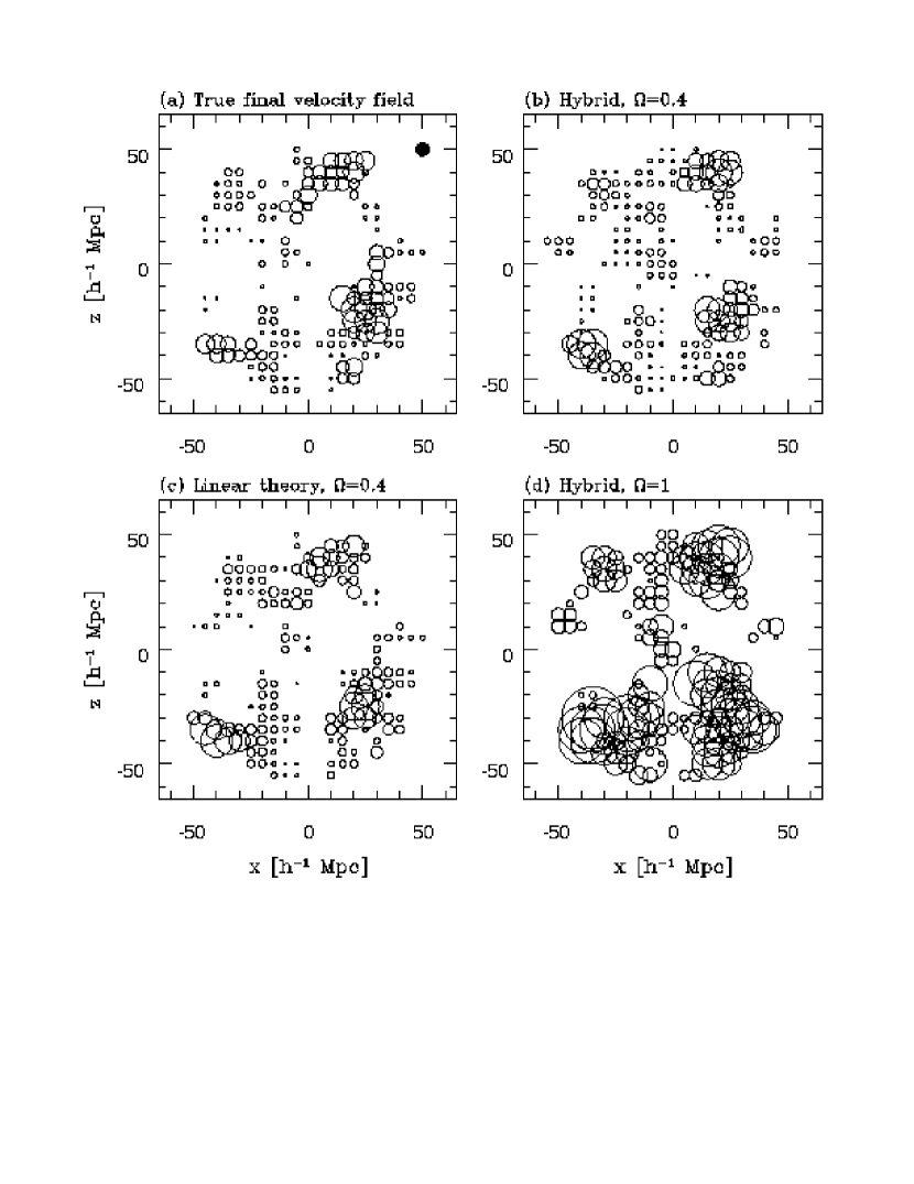
Figure 25: Velocity dispersion field of the true and reconstructed galaxy distributions for the mock PSCZ catalog. (a) True mock PSCZ catalog. (b) Reconstructed galaxy distribution assuming $\Omega=0.4$ (c) Linear theory prediction for $\Omega=0.4$ (d) Reconstructed galaxy distribution assuming $\Omega=1$ . We compute the velocity dispersion only if there are at least four galaxies within $5h^{-1}$Mpc of the field point. The radius of the filled circle centered at (50,50) in panel (a) corresponds to a velocity dispersion of 400 kms^-1.

4.3 Reconstruction of a Mock ORS Catalog

The ORS (Santiago et al. (1995)) is a redshift survey of optically selected galaxies covering about $98\%$ of the sky with Galactic latitude $|b|>20^{\circ}$. It is drawn from three different catalogs, the Uppsala Galaxy Catalog (UGC), the European Southern Observatory Galaxy Catalog (ESO), and the Extension to the Southern Galaxy Catalog (ESGC). It has 2 subcatalogs, one magnitude-limited subsample complete to a $B$ magnitude of 14.5 and another subcatalog complete to a $B$ major axis diameter of $1.9^{\prime}$. There are about $8500$ galaxies in the catalog distributed over a solid angle of 8.09sr, with the magnitude-limited subsample containing about $5700$ galaxies. We make a mock ORS catalog using the same mass distribution and Local Group observer used to create the PSCZ mock catalog. We first select “galaxies” from this mass distribution using the power law biasing scheme described by equation (13), so that the rms fluctuation amplitude of the resulting galaxy distribution is $\sigma_{8g}=1.1\simeq 1.5\sigma_{8m}$. We then select a volume limited subsample out to a radius of $40h^{-1}$Mpc so that the average density of galaxies in this volume is $0.008h^{3}$Mpc^-3. We include an outer magnitude limited sample up to a radius of $60h^{-1}$Mpc, where the selection function decreases as $\phi(r)\propto r^{-3}$, and we exclude all galaxies in a $40^{\circ}$ wedge about the Local Group to mimic the survey’s Galactic plane cut. Finally, we “observe” this galaxy distribution in redshift space in the frame of the Local Group observer.

We reconstruct this mock ORS catalog using the hybrid method as applied to biased galaxy distributions. The details of this reconstruction are similar to those of the mock PSCZ catalog reconstruction. The differences are: (1) After correcting for redshift space distortions using the method described in §4.2, we map the real space galaxy density field to an empirically determined mass PDF with the appropriate $\sigma_{8m}$. (2) We fix the amplitude of fluctuations in the reconstructed initial density field so that $\sigma_{8m}=\sigma_{8g}/b$. (3) We choose “galaxies” from the reconstructed mass distribution using the power law biasing relation defined by equation (13). We set the parameters $A$ and $B$ of this relation so that the galaxy density is $n_{g}=0.008h^{3}\;{\rm Mpc}^{-3}$ and the rms galaxy fluctuation in redshift space $\sigma_{8g}$ matches that of the input mock catalog.

We present the results of the reconstruction analysis of the mock ORS catalog in Figures 26 to 33, in the same manner as for the mock PSCZ catalog reconstruction. We show the density fields and the galaxy distributions in the same slice as for the mock PSCZ catalog. Figure 26 shows the isodensity contours of the initial density field. Although the gross features are recovered, the recovery is generally poor, especially near the survey boundaries. This poor recovery could in principle reflect either the small outer radius limit ($40{h^{-1}\;{\rm Mpc}}$ vs. $55{h^{-1}\;{\rm Mpc}}$ for PSCZ) or the large angular mask of the mock ORS catalog. To check which of the two effects is dominant, we reconstructed the mock ORS catalog assuming a smaller angular mask. We found that the initial density field was recovered very well and the correlation between the true and reconstructed fields was comparable to that for the mock PSCZ reconstruction. This suggests that we could significantly improve the reconstruction of the ORS catalog by filling in the large Galactic plane mask with the density field mapped by the PSCZ catalog. We should of course, normalize the PSCZ density field to have the same fluctuation amplitude as the ORS density fluctuations before filling in this region. We have not followed this filling-in procedure here, but we may do so when analyzing the real ORS data.

We show the scatter plot of the true and reconstructed initial and final density fields in Figures 27a and 27b respectively. The weak correlation between the true and recovered initial density fields quantifies the poor recovery seen in Figure 26. Figure 28 shows the power spectrum of the true initial density field (dotted line) and of the reconstructed initial fields after the power restoration and amplitude matching procedures. The amplitudes of the reconstructed initial density fields are normalized so that $\sigma_{8m}=\sigma_{8g}/b=0.75$. This normalization is accurate essentially by construction. However, although the overall slopes of the recovered power spectra are correct, there are substantial oscillations in the recovered power spectrum that are not present in the true initial density field.

Figure 26: Contours in a slice of the (a) true and (b) reconstructed initial density fields for the mock ORS catalog in the same format as Fig. 16. A slice through the galaxy distribution obtained by evolving the field in (a), and selecting galaxies in a biased manner is shown in Fig. 29a.

Figure 27: (a) Cell by cell comparison of the hybrid reconstructed initial density contrast $(\frac{\delta}{\sigma})_{r}$ to the true initial density contrast $(\frac{\delta}{\sigma})_{i}$ for the mock ORS catalog. (b) Comparison of the reconstructed final density contrast $(\frac{\delta}{\sigma})_{r}$ to the true final density contrast $(\frac{\delta}{\sigma})_{f}$, in redshift space. All the density fields are smoothed using a Gaussian filter of radius 3$h^{-1}$Mpc and scaled by the rms fluctuation $\sigma$. The linear correlation coefficient $r$ is indicated above each panel.

Figure 28: Power spectrum of the true initial density field of the mock ORS survey(dotted line) and the normalized hybrid reconstructed density field recovered for $\Omega=0.4$ (the correct value, solid line) and for $\Omega=1$ (incorrect value, dashed line). The arrows show the smallest wavenumber that corresponds to the survey size ($k_{\rm surv}=2\pi/2r_{\rm in}=0.078\ h$Mpc^-1) and the maximum wavenumber $k_{\rm corr}=15k_{f}=0.471\ h$Mpc^-1 beyond which random phase waves are added to the reconstructed field.

Figure 29 shows the galaxy distributions of the mock ORS catalog and its reconstruction assuming $\Omega=0.4$, in real space (panels a and b) and redshift space (panels c and d). Here again, as in the reconstruction of the mock PSCZ catalog, the filamentary structure running from $(x,z)=(-10,20)h^{-1}$Mpc to $(10,35)h^{-1}$Mpc is absent in the reconstruction. There are also a few spurious features that are present in the reconstruction alone, such as the clusters seen at $(x,z)=(20,35)h^{-1}$Mpc and $(-15,-15)h^{-1}$Mpc. The cluster at $(x,z)=(25,-20)h^{-1}$Mpc, although recovered at the proper location, appears very rich in the reconstruction. These features are also seen in redshift space, where the clusters have prominent “Fingers of God” in the reconstruction but not in the true galaxy distribution. We also see that the reconstructed galaxy distribution appears more dynamically evolved than the true galaxy distribution, although the final $\sigma_{8g}$ of the two redshift space galaxy distributions are identical and the power spectra are similar. We show the multiplicities and velocity dispersions of clusters in panels (a) and (b) of Figure 30. Although the cluster multiplicities are similar for the $\Omega=0.4$ and $\Omega=1$ reconstructions, the cluster velocity dispersions are significantly higher than the true values for the $\Omega=1$ reconstruction.

Figure 29: Final galaxy distributions for mock ORS catalog in the region $-20<y<20h^{-1}$Mpc. (a) True final galaxy distribution in real space. (b) Final galaxy distribution of hybrid reconstruction in real space. (c) True final galaxy distribution in redshift space. (d) Final galaxy distribution of hybrid reconstruction in redshift space.

Figure 30: Comparison of (a) cluster multiplicities and (b) cluster velocity dispersions for the mock ORS catalog reconstruction. Squares parallel to either axis represent clusters present in that galaxy distribution alone. Open symbols show the reconstruction with $\Omega=0.4$ (correct value), and the filled symbols show a reconstruction with $\Omega=1$.

Figure 31 shows the two-point correlation functions $\xi(s,\mu)$ of the mock ORS catalog and its reconstructions after compressing the clusters. The various symbols have the same meaning as in Figure 21. The large scale clustering amplification along the line of sight is much stronger for the $\Omega=1$ reconstruction compared to that of the true distribution and the $\Omega=0.4$ reconstruction. Figure 32 shows the fractional difference between the mean and the observed correlation functions for the ORS reconstruction in a manner similar to Figure 22 for the PSCZ catalog. The mean correlation function $\overline{\xi(s,\mu)}$ and the cosmic variance band are computed from an ensemble of 20 independent mock ORS catalogs. This cosmic variance band is broader than that for the PSCZ catalog in Figure 22 because the ORS catalog surveys a smaller volume and employs a sparser sampling (at the chosen limiting radius). We see that the $\xi(s,\mu)$ for the reconstruction with the correct assumption of $\Omega=0.4$ always matches the true $\xi(s,\mu)$ to much better than the cosmic variance limit. On the other hand, the $\Omega=1$ reconstruction has a significantly higher degree of angular anisotropy and is a poor match to the true anisotropies. This shows that we can effectively use the large scale amplification in the correlation function for $\mu\geq 0.7$ as a good diagnostic of $\Omega$ (or at least $\beta$), despite the errors caused by the angular mask of the ORS.

Figure 31: Correlation functions of the mock ORS catalog and its reconstructions after compressing the clusters. The galaxy pairs contributing to different panels have different orientations relative to the line of sight, $\mu=\cos(\theta)$. The filled circles show the real space correlation function of the mock catalog and are the same in all panels. The dotted line shows the redshift space correlation function of the mock catalog. The solid line shows the redshift space correlation function for a hybrid reconstruction using $\Omega=0.4$ (the correct value), while the dashed line is for a reconstruction with $\Omega=1$.

Figure 32: Fractional difference between the correlation function of the reconstruction and the true correlation function in redshift space for the mock ORS catalog. The mean correlation function $\bar{\xi}$ and the cosmic variance band (shaded region) are computed from an ensemble of 20 independent mock ORS catalogs. The filled squares show the redshift space correlation for the mock catalog. The solid and dashed lines show the redshift space correlation function for hybrid reconstructions assuming $\Omega=0.4$ and $\Omega=1$, respectively.

We computed the nearest neighbor distribution for the mock ORS catalog and its reconstructions assuming $\Omega=0.4$ and $\Omega=1$, in the same manner as described for the mock PSCZ catalog. We found that both the reconstructions recovered the nearest neighbor distribution of the input data quite accurately.

Figure 33 shows the $x$ and $z$ components of the velocity fields for the mock ORS catalog and its reconstructions. These fields are computed in the same manner as described for the mock PSCZ catalog, and the fields are plotted in that slice whose density contours are shown in Figure 26. The linear theory predicted velocity field is derived from the density contrast field $\delta_{m}$ that is obtained by dividing the real space galaxy density contrast field by the bias factor, i.e, from $\delta_{m}=\delta_{g}/b$. We find that the correct assumption reconstruction ($\Omega=0.4$) provides the best match to the true field in both the amplitude and the non-linear components. The linear theory velocity field does not reproduce well the small scale incoherent velocities, and the velocity field of the $\Omega=1$ reconstruction has a much higher amplitude and is very hot compared to the true field. We also computed the velocity dispersion field of the true and the reconstructed ORS catalogs in the same manner as for the PSCZ catalog. Here also, we found that both the amplitude and the spatial variation of this velocity dispersion is best recovered by the reconstruction that correctly assumes $\Omega=0.4$ and $b=1.5$.

Figure 33: Velocity fields of the true and reconstructed galaxy distributions for the mock ORS survey, averaged over a $5h^{-1}$Mpc top hat window. Only the $x$ and $z$ components of the velocity field in a slice through the center of the survey are shown. (a) Velocity field of the true mock ORS catalog. (b) Reconstructed velocity field using $\Omega=0.4$. (c) Linear theory prediction for $\Omega=0.4$. (d) Reconstructed velocity field using $\Omega=1$. The length of the dark arrow in the top right corner in panel (a) corresponds to 500 kms^-1.

4.4 Reconstruction with Incorrect Bias Factors

In all of the reconstructions of the mock catalogs shown so far, we have assumed that we know the correct value of the bias factor. This is not the situation when we reconstruct the observed redshift galaxy distributions. The anisotropy of $\xi(s,\mu)$ and the cluster velocity dispersions constrain most directly a parameter combination that is similar to $\beta$ (it is exactly equal to $\beta$ in the linear regime). Translating this to a constraint on $\Omega$ requires independent information about the bias factor. To check if we can constrain $\Omega$ and $b$ individually, we reconstructed the mock PSCZ and ORS catalogs with different assumptions about $\Omega$ and $b$. Apart from the cases considered above, we used other combinations of $\Omega$ and $b$ that have roughly the same $\beta$ as the respective mock catalogs. We do not show the results of these additional reconstructions in detail. Our main conclusions from these are:

(1)

The reconstruction with the correct assumption for $\Omega$ and $b$ always provides the best match to the input galaxy distribution.

(2)

Although the large scale clustering amplification depends only on $\beta$ in linear theory, we find that the fractional difference between the true and the reconstructed $\xi(s,\mu)$ is the smallest for the reconstruction with the correct $\Omega$ and $b$, when we compare in all the angular bins.

(3)

The nearest neighbor distributions computed using the transverse separations do not discriminate between the different assumptions about the bias factor for the mock PSCZ catalog reconstructions. The evolved structure is very similar for the range of $b$ considered. We do see a marginal difference of the expected direction in the nearest neighbor distributions of the mock ORS catalog reconstructions, although this difference may be too small to be detected at a reasonable confidence level.

(4)

The cluster velocity dispersions and the peculiar velocity field are primarily determined by the value of $\beta$.

5 DISCUSSION

In this paper, we have described and tested a hybrid reconstruction scheme that can be used to reconstruct the observed distribution of galaxies. When the galaxy distribution is an unbiased tracer of the mass distribution, this scheme consists of the steps (H1)-(H7) listed in §2.2. If the galaxy distribution is biased with respect to the underlying mass distribution, we replace the steps (H2) and (H6) by the steps (H2B) and (H6B).

A hybrid reconstruction using this method incorporates a number of assumptions. The need for these assumptions and their effects on the reconstruction are discussed at the beginning of §3. The most fundamental of these assumptions is the hypothesis that the primordial density fluctuations form a Gaussian random field, as predicted by simple inflation models for the origin of the fluctuations (Guth & Pi (1982); Hawking (1982); Starobinsky (1982); Bardeen, Steinhardt, & Turner (1983)). Other assumptions include the values of the density parameter $\Omega$ and the bias factor $b$ and the biasing model used to select galaxies from the evolved mass distribution. Given a redshift space galaxy distribution, we can reconstruct it using different combinations of the latter assumptions, within the general framework of Gaussian initial fluctuations. We can then use both local comparisons of structure and global statistical comparisons to check what combinations of the assumptions, if any, can best reproduce the input data. In application to observational data, these comparisons will enable us to test the validity of the different assumptions and to constrain the allowed ranges of cosmological parameters. If there is no reasonable combination of assumptions for which the reconstructed galaxy distribution accurately reproduces the input galaxy distribution, we will be forced to question the Gaussian assumption itself and explore alternative scenarios for the origin of structure.

We tested the hybrid reconstruction method on idealized galaxy distributions derived from the mass distributions of N-body simulations. We tested it on both unbiased and biased galaxy distributions. We also tested this reconstruction scheme on mock galaxy redshift catalogs that are designed to mimic the geometry and depth of the PSCZ and ORS surveys. In all these tests, we were primarily interested in checking whether the hybrid reconstruction method can accurately reproduce the input galaxy distribution for the correct set of assumptions and discriminate against incorrect assumptions. Our conclusions from these tests are as follows:

(1)

The hybrid method recovers the initial density fluctuations much better than either the Gaussianization or the dynamical scheme alone. The hybrid reconstructed galaxy distribution matches the local and global properties of the true input galaxy distribution more accurately than the galaxy distribution reconstructed by Gaussianization.

(2)

A reconstruction that incorporates correct assumptions about $\Omega$ and $b$ always yields the best match to the input data. Reconstructions with wrong assumptions about these parameters produce a galaxy distribution that is identifiably different from the input galaxy distribution.

(3)

The morphology of the true and reconstructed galaxy distributions can be used to constrain the bias factor $b$ independent of $\Omega$. For a fixed value of $\sigma_{8g}$, a biased galaxy distribution is less dynamically evolved than an unbiased one. This difference in the degree of dynamical evolution can be easily detected when comparing galaxy distributions with $b=1,b=2$, and $b=3$, using the nearest neighbor distribution. However, it may be difficult to distinguish between more moderate values of $b$, say between $b=1$ and $b=1.5$, using the PSCZ and the ORS catalogs. An uncertain form of the biasing relation between galaxies and mass will add another degree of freedom, extending the range of values of $b$ that provides acceptable reconstructions, and it will thus reduce the discriminatory power of the reconstruction method. However, we can expect improvements on this front, as we hope to get reasonable bias prescriptions through a better understanding of the galaxy formation process using hydrodynamical simulations (see, e.g., Cen & Ostriker (1992); Katz, Hernquist, & Weinberg (1992)).

(4)

Reconstruction allows the parameter $\beta=\Omega^{0.6}/b$ to be constrained more accurately than in conventional analyses of the anisotropy of the redshift space correlation because:

(a)

The reconstructed peculiar velocity field is fully non-linear and automatically includes the spatial variations of the non-linear component. Hence, while estimating $\beta$ from the angular anisotropies in $\xi(s,\mu)$, we are not restricted to the large scales where linear theory is a good approximation, but we instead use the correlation function information in the entire range of pair separations.

(b)

Using the correct assumptions for $\Omega$ and $b$ (or at least for the combination $\beta=\Omega^{0.6}/b$), we can reproduce the $\xi(s,\mu)$ of the input galaxy distribution more accurately than the cosmic variance band, because reconstructions automatically reproduce the orientations of large scale features that are the main source of noise in the purely statistical approach to redshift space distortions. This result is demonstrated in Figures 22 and 32 for the mock PSCZ and ORS surveys respectively.

(5)

Reconstruction predicts both the density and the fully non-linear velocity field starting from the redshift data alone. Thus, at any location in redshift space, we can construct a predicted distribution of the peculiar velocities of galaxies in its vicinity that is more accurate than that provided by linear theory. This prediction can be used to correct for the inhomogeneous Malmquist bias which plagues the estimates of $\beta$ from the comparison between observed density and velocity fields. It also has the potential to improve the performance of velocity-velocity comparisons (Willick et al. (1997); Willick & Strauss (1998)), as the velocity and velocity dispersion fields can be predicted more accurately.

(6)

The mock PSCZ catalog can be reconstructed more accurately than the mock ORS catalog. The difference primarily reflects the larger sky coverage of the PSCZ survey and not its greater depth. This result suggests that the reconstruction of the ORS catalog can be improved by filling in the large angular mask region with an appropriately normalized PSCZ density field. Alternatively, the initial density field recovered by the PSCZ catalog can be used to reconstruct the ORS catalog by using the forward evolution steps that are appropriate for a biased reconstruction. However, even without these modifications, the $\xi(s,\mu)$ of the reconstructed ORS catalog can match its input values to better than the cosmic variance limit, and the reconstructed velocity field is a better match to the true velocity field compared to the linear theory prediction. Thus, reconstruction will improve the ability of these surveys to constrain $\beta$ both from the analysis of clustering anisotropies and from peculiar velocity comparisons.

Reconstruction analysis is a complement to the statistical approach to large scale structure, not a replacement for it. Its strength lies in its ability to break the cosmic variance barrier and its ability to constrain $\Omega$ and $b$ by simultaneously using information from linear and non-linear scales. The penalty is that a reconstruction is not perfectly accurate even if it is based on correct assumptions, but the systematic errors of reconstruction on a particular data set can be calibrated using N-body mock catalogs. Reconstruction analysis can enhance the power of galaxy redshift surveys to constrain the density parameter and the relation between galaxies and mass and to test the hypothesis that large scale structure originated in the gravitational instability of Gaussian primordial density fluctuations.

References

- Bardeen, Steinhardt, & Turner (1983) Bardeen, J.M., Steinhardt, P.J., & Turner, M.S., 1983, Phys Rev D, 28,679
- Brown & Peebles (1987) Brown, M.E., & Peebles, P.J.E., 1987, ApJ, 317, 588
- Canavezes et al. (1998) Canavezes, A., et al. 1998, MNRAS, in press (astro-ph/9712228)
- Cen & Ostriker (1993) Cen, R., & Ostriker, J. 1993, ApJ, 417, 415
- Cen & Ostriker (1992) Cen, R., & Ostriker, J. 1992, ApJ, 399, L113
- Cole, Fisher, & Weinberg (1994) Cole, S., Fisher, K.B., & Weinberg, D.H. 1994, MNRAS, 267, 785
- Cole, Fisher, & Weinberg (1995) Cole, S., Fisher, K.B., & Weinberg, D.H 1995, MNRAS, 275 515
- Cole et al. (1997) Cole, S., Weinberg, D.H., Frenk, C.S., & Ratra, B. 1997, MNRAS, 289, 37
- Croft & Gaztañaga (1997) Croft, R.A.C., & Gaztañaga, E. 1997, MNRAS, 285, 793
- Davis & Peebles (1983) Davis, M., & Peebles, P.J.E. 1983, ApJ, 267, 465
- Davis et al. (1985) Davis, M., Efstathiou, G., Frenk, C.S, & White, S.D.M. 1985, ApJ, 292,371
- Efstathiou, Bond, & White (1992) Efstathiou, G., Bond, J.R., & White, S.D.M 1992, MNRAS, 258, 1P
- Eke, Cole, & Frenk (1996) Eke, V.R, Cole, S., & Frenk, C.S. 1996, MNRAS, 282, 263
- Fan, Bahcall, & Cen (1997) Fan, X., Bahcall, N.A., & Cen, R. 1997, ApJ, 490, L123
- Fisher et al. (1994) Fisher, K.B., Davis, M., Strauss, M.A., Yahil, A., & Huchra, J. 1994, MNRAS, 266, 50
- Fisher et al. (1995) Fisher, K.B., Huchra, J., Davis, M., Strauss, M.A., Yahil, A., & Schlegel, D. 1995, ApJS, 100, 69
- (17) Giavalisco, M., Mancinelli, B., Mancinelli, P.J., & Yahil, A. 1993, ApJ, 411, 9
- (18) Gramann, M. 1993a, ApJ, 405, 449
- (19) Gramann, M. 1993b, ApJ, 405, L47
- Gramann, Cen, & Gott (1994) Gramann, M., Cen, R., & Gott, R.J. 1994, ApJ, 425, 382
- Guth & Pi (1982) Guth, A.H., & Pi, S.Y. 1982, Phys Rev Let, 49, 1110
- (22) Hamilton, A.J.S. 1993a, ApJ, 406, L47
- (23) Hamilton, A.J.S. 1993b, ApJ, 417, 19
- Hawking (1982) Hawking, S.W. 1982, Physics Letters, 115, 295
- Huchra & Geller (1982) Huchra, J. P., & Geller, M. J. 1982, ApJ, 257, 423
- Hudson et al. (1995) Hudson, M.J., Dekel, A., Courteau, S., Faber, S.M., & Willick, J.A. 1995, MNRAS, 274, 305
- Kaiser (1987) Kaiser, N. 1987, MNRAS, 227, 1
- Katz, Hernquist, & Weinberg (1992) Katz, N., Hernquist, L., & Weinberg, D. H. 1992, ApJ, 399, L109
- Kolatt et al. (1996) Kolatt, T., Dekel, A., Ganon, G., & Willick, J.A. 1996, ApJ, 458, 419
- Lahav, Nemiroff, & Piran (1990) Lahav, O., Nemiroff, R.J., & Piran, T. 1990, ApJ, 350, 119
- Lilje & Efstathiou (1989) Lilje, P.B., & Efstathiou, G. 1989, MNRAS, 236, 851
- (32) Little, B., Weinberg, D.H, & Park, C. 1991, MNRAS, 253, 295 (LWP)
- Loveday et al. (1996) Loveday, J., Efstathiou, G., Maddox, S.J, & Peterson B.A. 1996, ApJ, 468,1
- Mann, Peacock, & Heavens (1998) Mann, R.G., Peacock, J.A, & Heavens, A.F. 1998, MNRAS, 293, 209
- Maddox et al. (1990) Maddox, S.J.M., Efstathiou, G., Sutherland, W.J, & Loveday, J. 1990, MNRAS, 242,43
- Melott, Weinberg, & Gott (1988) Melott, A.L., Weinberg, D.H., & Gott, R.J. 1988, ApJ, 328, 50
- Melott & Dominik (1993) Melott, A.L., & Dominik, K.G. 1993, ApJS, 86, 1
- Moore, Frenk, & White (1993) Moore, B., Frenk, C.S., & White, S.D.M. 1993, MNRAS, 261, 827
- Nolthenius & White (1987) Nolthenius, R., & White, S.D.M 1987, MNRAS, 235, 505
- Nusser et al. (1991) Nusser, A., Dekel, A., Bertschinger, E., & Blumenthal, G. 1991, ApJ, 379, 6
- Nusser & Colberg (1997) Nusser, A., & Colberg, J. M. 1997, MNRAS, 294, 457
- Nusser & Dekel (1992) Nusser, A., & Dekel, A. 1992, ApJ, 391, 443
- Nusser, Dekel, & Yahil (1995) Nusser, A., Dekel, A., & Yahil, A. 1995, ApJ, 449, 439
- Park, C. (1990) Park, C. 1990, Ph.D Thesis, Princeton University
- Peacock & Dodds (1994) Peacock, J.A., & Dodds, S.J. 1994, MNRAS, 267, 1020
- Peebles (1980) Peebles, P.J.E. 1980, The Large Scale Structure of the Universe, (Princeton: Princeton Univ. Press)
- Peebles (1989) Peebles, P.J.E. 1989, ApJ, 344, L53
- Ryden & Gramann (1991) Ryden, B., & Gramann, M. 1991, ApJ, 383, L33
- Sandage (1986) Sandage, A. 1986, ApJ, 301, 1
- Santiago et al. (1995) Santiago, B.X., Strauss, M.A., Lahav, O., Davis, M., Dressler, A., & Huchra, J.P. 1995, ApJ, 446, 457
- Santiago et al. (1996) Santiago, B.X., Strauss, M.A., Lahav, O., Davis, M., Dressler, A., & Huchra, J.P. 1996, ApJ, 461, 38
- Sargent & Turner (1977) Sargent, W. W., & Turner, E. L. 1977, ApJ, 212, L3
- Saunders, Rowan-Robinson, & Lawrence (1992) Saunders W., Rowan-Robinson, M., & Lawrence, A. 1992, MNRAS, 258, 134
- Saunders et al. (1995) Saunders W., Sutherland, W., Efstathiou, G., & Tadros, H. 1995, in Wide Field Spectroscopy and the Distant Universe, eds. S.J.Maddox & Aragón-Salamanca, A., (Singapore: World Scientific), p. 88
- Shaya, Peebles, & Tully (1995) Shaya, E.J., Peebles, P.J.E., & Tully, R.B. 1995 ApJ, 454, 15
- Sigad et al. (1997) Sigad, Y., Eldar, A., Dekel, A., Strauss, M.A., & Yahil, A. 1998, ApJ, 495, in press (astro-ph 9708141)
- Starobinsky (1982) Starobinsky, A. A. 1982, Phys Lett B, 117, 175
- Weinberg (1992) Weinberg, D.H. 1992, MNRAS, 254, 315 (W92)
- Weinberg & Cole (1992) Weinberg, D.H., & Cole, S. 1992, MNRAS, 259, 652
- Weinberg, Hernquist, & Katz (1997) Weinberg, D.H., Hernquist, L., & Katz, N. 1997, ApJ, 477, 8
- Weinberg & Gunn (1990) Weinberg, D.H., & Gunn, J.E. 1990, MNRAS, 247, 260
- White et al. (1987) White, S.D.M., Frenk, C.S., Davis, M., & Efstathiou, G. 1987, ApJ, 313, 505
- White, Efstathiou, & Frenk (1993) White, S.D.M., Efstathiou, G., & Frenk, C.S. 1993, MNRAS, 262, 1023
- Willick & Strauss (1998) Willick, J. A., & Strauss, M. A. 1998, ApJ, submitted (astro-ph/9801307)
- Willick et al. (1997) Willick, J.A., Strauss, M.A., Dekel, A., & Kolatt, T. 1997, ApJ, 486, 629
- Yahil et al. (1991) Yahil, A., Strauss, M.A., Davis, M., & Huchra, J.P. 1991, ApJ, 372, 380
- Zel’dovich (1970) Zel’dovich, Ya. B. 1970 A&A, 5, 84