Gravothermal Catastrophe in Anisotropic Spherical Systems

Abstract

In this paper we investigate the gravothermal instability of spherical stellar systems endowed with a radially anisotropic velocity distribution. We focus our attention on the effects of anisotropy on the conditions for the onset of the instability and in particular we study the dependence of the spatial structure of critical models on the amount of anisotropy present in a system. The investigation has been carried out by the method of linear series which has already been used in the past to study the gravothermal instability of isotropic systems.

We consider models described by King, Wilson and Woolley-Dickens distribution functions. In the case of King and Woolley-Dickens models, our results show that, for quite a wide range of amount of anisotropy in the system, the critical value of the concentration of the system (defined as the ratio of the tidal to the King core radius of the system) is approximately constant and equal to the corresponding value for isotropic systems. Only for very anisotropic systems the critical value of the concentration starts to change and it decreases significantly as the anisotropy increases and penetrates the inner parts of the system. For Wilson models the decrease of the concentration of critical models is preceded by an intermediate regime in which critical concentration increases, it reaches a maximum and then it starts to decrease. The critical value of the central potential always decreases as the anisotropy increases.

1 Introduction

It is well known that the phenomenon of gravothermal instability is strictly related to the property of self-gravitating systems of having a negative specific heat. In 1962 Antonov showed that there is no state characterized by a local maximum in the entropy for stellar systems with fixed mass and energy, contained in a spherical box with radius greater than the critical value $r_{\rm crit}=-0.335({GM^{2}}/{E})$ where $M$ is the total mass of the system and $E$ its total energy. Lynden-Bell and Wood (1968) interpreted this result in their pioneering work on the stability of isotropic isothermal stellar systems truncated in radius, establishing the conditions for the onset of the phenomenon, called then gravothermal catastrophe. The investigation was carried out by means of the method of linear series formulated for the first time by Poincaré (1885); this technique is connected with the study of global stability of the equilibria of a generic system.

In the case of isothermal configurations, the equilibrium states in the presence of encounters are determined by finding the conditions for a maximum of the total entropy $S$, keeping fixed the total energy and mass, $E$ and $M$, of the system. The phase-space distribution function that describes a system under these requirements turns out to be the Maxwell-Boltzmann function,

$$f(\varepsilon)=A\>e^{-\beta\varepsilon},$$ (1)

where

$$\varepsilon={1\over 2}{v^{2}}+\Phi(r)$$ (2)

is the energy per unit mass of single stars, $\beta$ is the inverse of the “temperature”, $A$ is a normalization constant and $\Phi(r)$ is the self-consistent gravitational potential obtained by solving the Poisson equation. Lynden-Bell and Wood focussed their attention on the study of the stability of a system against perturbations keeping constant, besides the total mass and energy, the radius of the system also. The critical value of the concentration of the system, as measured by the ratio of the central density, $\rho_{\rm c}$, to the average density inside the boundary of the system, $\rho_{\rm b}$, is equal to $\rho_{\rm c}/\rho_{\rm b}=709$ which coincides with the result found by Antonov.

An analogous investigation was later carried out by Katz (1978, 1980) for more realistic models of stellar clusters. Katz studied the gravothermal instability of King (1965), Woolley-Dickens (1961) and Wilson (1975) models, which are all characterized by distribution functions with a cut-off in the energy space. In this case, the study of the stability was realized keeping fixed the total mass, the total energy and the multiplicative normalization parameter $A$ which reflects the indetermination in the zero of the chemical potential (see the appendix of Katz (1980) for the discussion on the motivation for this choice). In these cases, the onset of gravothermal instability occurs for the following values of the central dimensionless relative potential, $\tilde{\Psi}_{\rm c}\equiv\beta\Psi_{\rm c}$,

$$\begin{array}[]{lll}1)\;\tilde{\Psi}_{\rm c}=7.65,&&Woolley-Dickens\;models,\\ 2)\;\tilde{\Psi}_{\rm c}=7.40,&&King\;models,\\ 3)\;\tilde{\Psi}_{\rm c}=6.67,&&Wilson\;models.\end{array}$$ (6)

Taking anisotropy in the velocity distribution into account is an essential step in order to improve the reliability of energy-truncated models to better describe the structure and evolution of clusters. The important role played by anisotropy has been recognized since the dawn of the study of globular clusters (Woolley & Robertson, 1956). The main goal of the present paper is that of extending the study of gravothermal instability to spherical systems endowed with an anisotropic velocity distribution and determining the dependence of the critical value of $\tilde{\Psi}_{\rm c}$ on the amount of anisotropy present in the systems. We point out that our analysis is meant to provide only a general indication of the role of radial anisotropy on the onset of gravothermal instability, providing a simple and straightforward estimate of its effect as measured by the critical value of the central potential and of the concentration of the system (given by the ratio of the total radius of the system to the King core radius). A much deeper insight in the collisional evolution of anisotropic systems can be obtained only by other methods of investigation such as $N$-body simulations, integration of the Fokker-Planck equation and gaseous models (see e.g. Takahashi 1995, 1996, Takahashi, Lee & Inagaki 1997, Spurzem & Takahashi 1995, Giersz & Spurzem 1994, Bettwieser & Spurzem 1986, Giersz & Heggie 1994a,b, 1996, 1997, Louis & Spurzem 1991, Spurzem 1991, Spurzem & Aarseth 1996, for some interesting and detailed investigations on the evolution of anisotropic stellar systems). In Sects. 3.3 and 4, we compare the global indications resulting from the present study with the specific findings of some of the most recent works cited above.

The scheme of the paper is the following: in Section 2 we summarize the main properties of these models, in Section 3 we study their stability by means of the method of linear series discussing the results and, finally, in Section 4 we summarize the main conclusions.

2 Anisotropic models

The relevance of an anisotropic model for the description of real stellar systems arises when studying the first periods of life of stellar systems: it is possible to demonstrate that, at the end of the process of the violent relaxation (Lynden-Bell, 1967), stellar systems are anisotropic because they still have stars mainly distributed on radial orbits, and, although they tend to relax and become isotropic on a time scale which is of the order of the binary relaxation time (see, e.g., Binney & Tremaine, 1987), if the conditions for the onset of the gravothermal instability take place before their total isotropization, anisotropy cannot be left out of consideration. It must be remarked that, in evolving systems like globular clusters, anisotropy is not simply removed by relaxation. Rather, it is even increased in the halo, due to the high energy stars coming from the strong relaxing core (Takahashi 1996) and it is also expected to gradually penetrate into the inner regions as the core collapses. The situation is different for tidally truncated systems in which stars can escape at a significant rate from the cluster: in this case it has been shown (Giersz & Heggie 1997, Takahashi et al. 1997) that anisotropy production can be partially or completely balanced by the evaporation of stars which would occur preferentially for stars on radial orbits.

In any case, if primordial anisotropy changes the conditions for the onset of gravothermal instability, this can also have important consequences on the subsequent evolution of anisotropy itself. In the present Section we describe the properties of the anisotropic variants of the energy-truncated models mentioned above, which, in the subsequent one, will be submitted to the analysis of gravothermal stability.

2.1 Description of anisotropic spherical models

Following arguments similar to those of Tremaine (1986) in the discussion of the process of violent relaxation, the distribution functions introduced to describe anisotropic systems are obtained by multiplying by a factor of the form

$$k(L^{2})\equiv e^{-\frac{L^{2}}{2\sigma^{2}r_{\rm a}^{2}}}$$ (7)

the isotropic King, Woolley-Dickens and Wilson distribution functions, which therefore can be written in the form

$$\begin{array}[]{lll}1)\;f_{WD}(\epsilon,L^{2})=A\>e^{-\frac{\epsilon}{\sigma^{2}}}\>e^{-\frac{L^{2}}{2\sigma^{2}r_{\rm a}^{2}}},\\ 2)\;f_{K}(\epsilon,L^{2})=A\>\left(e^{-\frac{\epsilon}{\sigma^{2}}}-1\right)\>e^{-\frac{L^{2}}{2\sigma^{2}r_{\rm a}^{2}}},\\ 3)\;f_{W}(\epsilon,L^{2})=A\>\left(e^{-\frac{\epsilon}{\sigma^{2}}}+\frac{\epsilon}{\sigma^{2}}-1\right)\>e^{-\frac{L^{2}}{2\sigma^{2}r_{\rm a}^{2}}}.\end{array}$$ (11)

The above definitions hold for $\epsilon<0$, while it is assumed that $f(\epsilon)=0$ for $\epsilon>0$. In each distribution function, the parameter $\beta$ has been substituted with the inverse of the isothermal velocity scale $\sigma^{2}$. The dependence of the functions on the square of the angular momentum $L$ ensures the spherical symmetry of the global properties of the models. In (7), $r_{\rm a}$ is the anisotropy radius that represents the value of the radius beyond which the orbits start to be mainly radial. The distribution function $f_{K}(\epsilon,L^{2})$ is usually known as Michie model (Binney & Tremaine, 1987), whereas $f_{W}(\epsilon,L^{2})$ is simply the spherically symmetric version of the generic function introduced by Wilson (1975) himself.

In order to perform the integration of these models, we define the following dimensionless quantities:

$$x\equiv\frac{r}{r_{K}},\hskip 28.45274pt\tilde{v}\equiv\frac{v}{\sigma},$$ (12)

so that

$$\tilde{\epsilon}\equiv\frac{\epsilon}{\sigma^{2}}={1\over 2}{\tilde{v}}^{2}+\tilde{\Phi},\hskip 14.22636pt\tilde{\Phi}\equiv\frac{\Phi}{\sigma^{2}}.$$ (13)

In (12),

$$r_{\rm K}=\frac{3\sigma}{\sqrt{4\pi G\rho_{\rm c}}}$$ (14)

is the King radius and gives the length scale. Calling $r_{\rm t}$ the tidal radius of the system, so that $x_{\rm t}=r_{\rm t}/r_{\rm K}$, the self-consistent relative potential

$$\tilde{\Psi}(x)=-\tilde{\Phi}(x)+\tilde{\Phi}(x_{\rm t})$$ (15)

and, from it, the physical properties of the models, is obtained by solving the Poisson equation which can be written in terms of the dimensionless quantities introduced in (12) and (13) as:

$$\frac{1}{x^{2}}\>\frac{d}{dx}\>\left(x^{2}\>\frac{d\tilde{\Psi}}{dx}\right)=\frac{d^{2}\tilde{\Psi}}{dx^{2}}+\frac{2}{x}\>\frac{d\tilde{\Psi}}{dx}=$$

$$=\frac{4\pi Gr_{\rm K}^{2}}{\sigma^{2}}\rho(\tilde{\Psi}(x),x))=-9\>\frac{\rho(\tilde{\Psi}(x),x)}{\rho_{\rm c}}$$ (16)

where the last equality comes from the substitution of $r_{\rm K}$ with its explicit expression. The related Cauchy’s problem is then solved with initial conditions $\tilde{\Psi}(0)=\tilde{\Psi}_{\rm c}$ and $\tilde{\Psi}^{\prime}(0)=0$.

The degree of anisotropy of a given model is parametrized by the dimensionless anisotropy radius

$$\gamma\equiv\frac{r_{\rm a}}{r_{\rm K}}.$$ (17)

We have carried out the integration of anisotropic Woolley-Dickens, King and Wilson models by selecting different values of the anisotropy parameter $\gamma$ and of the central potential $\tilde{\Psi}_{\rm c}$. $\gamma$ has been chosen to range from almost isotropic configurations ($\gamma=100$) up to highly anisotropic models ($\gamma=0.3$). Models with higher values of $\tilde{\Psi}_{\rm c}$ tend all to the singular isothermal sphere; however, highly concentrated models, pose a certain constraint on the range allowed to the anisotropy parameter. On the other hand, following arguments analogous to those in Merritt et al. (1989), it can be shown that singular models with a completely radial distribution display unphysical behaviour.

Figure 1: $\gamma_{\rm BS}$ versus the dimensionless central potential $\tilde{\Psi}_{\rm c}$ for the first unbounded Woolley-Dickens (a), King (b) and Wilson model (c).

2.2 Infinite models

An interesting feature of these models is the existence of definite pairs of values ($\gamma,\tilde{\Psi}_{\rm c}$) that identify unbounded models, i.e. models with an infinite radius. In fact, there is a critical value of the central potential, depending on the degree of anisotropy characterising each model, beyond which we have $r_{\rm t}\rightarrow\infty$ for every $\gamma$; this happens even though the distribution functions used for the description of these models are energy-truncated and the corresponding isotropic configurations are always bounded. Such remarkable peculiarity is common to all anisotropic models, regardless of the form of the dependence on the energy of the functions (11).

Following Stiavelli & Bertin (1985) we consider the parameter

$$\gamma_{\rm BS}\equiv\frac{1}{4\pi GA\sigma r_{\rm a}^{2}}.$$ (18)

This parameter is related to our anisotropy parameter through the following relation:

$$\gamma_{\rm BS}=\frac{\rho_{\rm c}}{9\sigma^{3}A\gamma^{2}}.$$ (19)

In Fig. 1 we have plotted $\gamma_{\rm BS}$ versus $\tilde{\Psi}_{\rm c}$ for the anisotropic Woolley-Dickens, King and Wilson models having an infinite radius. These models are singled out identifying, along the sequence at given $\tilde{\Psi}_{\rm c}$ parametrized by $\gamma_{\rm BS}$, the first system for which the relative potential goes as $1/x$ at large radius.

It is evident that the behaviour is the same of that shown in the paper by Stiavelli & Bertin (1985) and thus it seems that this characteristic is common to all the spherical anisotropic models having a dependence on the angular momentum of the kind $e^{-L^{2}}$, regardless to the form of the energy distribution.

Note that not all these unbounded models are relevant to model real physical systems; in fact, while the total dimensionless mass of infinite Wilson and Bertin-Stiavelli models is finite, it diverges for anisotropic Woolley-Dickens and King models, making the latter models useful only for those values of $\tilde{\Psi}_{\rm c}$ and $\gamma_{\rm BS}$ which lead to a finite-size system.

3 Gravothermal instability of spherical anisotropic models

3.1 Linear series of equilibrium

The investigation of the gravothermal stability of the models discussed in Section 2 has been carried out by means of the method of linear series. This approach, introduced by Poincaré in 1885, is based on the study of global stability of the equilibrium states of a generic system. In many stationary problems, the description of a system depends on some parameter other than the generalized coordinates $q_{i}$ ($i=1,\dots,n$) in terms of which we describe the configuration of the system. If we call $\mu$ this parameter and $U$ the potential energy of the system, the condition for the existence of an equilibrium is that the tangent plane to the $n$-dimensional surface

$$U(\mu,q_{i})=\rm const$$ (20)

in the equilibrium point is perpendicular to the $\mu$ axis. For every fixed value of $\mu$ in appropriate ranges, we obtain an equilibrium configuration. Therefore, if we call $q_{i}^{0}$ this configuration, we have

$$q_{i}^{0}=q_{i}^{0}(\mu).$$ (21)

These points are called level points and, by varying the value of the parameter $\mu$, they form a curve called linear series (Poincaré, 1885). To verify the stability of these equilibria, we restrict our attention to a plane $\mu=\rm const$. In statics, the condition for an equilibrium to be stable is that the potential energy $U$ in that point has a minimum. In our case, this statement means that a point on the linear series (21) represents a stable configuration only if all the different vertical sections of the surface $U=$ constant across that point are turned towards the direction of decreasing $U$.

It is possible to prove (see, e.g., Jeans, 1928) that every change in the stability of a system corresponds to an extremum of the linear series. Accordingly, the investigation of the stability of a self-gravitating system with respect to the gravothermal catastrophe, is accomplished locating the first critical point on a suitably parametrized linear series. This is a sequence of equilibrium systems with appropriate constraints insuring that the perturbation implicit in the stability analysis, keeps fixed the relevant physical quantities of the system. The critical value of the parameter identifies the transition from stability to instability.

3.2 Choice of the constraints

In the problem we are investigating, since the distribution functions (11) depend on the three parameters $A$, $\sigma$, $\gamma$ (or $r_{\rm a}$) and on the central potential $\Psi_{\rm c}$, we will have to fix, in agreement with the theory, three quantities belonging to the particular model under consideration and let a fourth quantity vary as a function of a parameter that is able to describe such model in a unique way. Besides keeping fixed the total mass of the system and the parameter $A$ (see Katz, 1980, for a discussion about this constraint), the parameter $\gamma$ has been held constant and we will investigate the stability by means of the curves of the total energy of the system versus the central dimensionless potential. Our results will thus be relevant for perturbations in which $A$, $M$, $E$ and $\gamma$ remain constant.

As for the first three quantities we thus adopt the same constraints used in the study of stability of isotropic systems by Katz (1980). For what concerns the fourth quantity, it is worth noting that the anisotropy parameter $\gamma$ is only one of the possible choices, but other quantities related to the anisotropy of the configurations could be held constant along the equilibrium sequences. We could not find any convincing physical criterion in favor of one particular choice and the parameter $\gamma$ chosen has the advantage of allowing a straghtforward implementation of the calculation.

While it would be clearly desirable that the arguments supporting the choices of the constraints (in particular the choice of keeping $A$ fixed) were substantiated by a more rigorous theory on the statistical mechanics of the gravitating systems, there are, however, several independent evidences supporting the validity of the basis of the present approach. In fact, in the case of isotropic King models, the results of some Fokker-Planck simulations (which are free of any assumption of the kind made in our investigation) by Wiyanto et al. (1985) have confirmed with good accuracy the instability limit found by Katz (1980) and the Fokker-Planck simulations by Cohn (1980) have shown that, for Plummer models also, the value of the central dimensionless potential at the onset of gravothermal instability is similar to that found by Katz. Moreover, it is worth emphasizing that the choice of the third parameter to be kept constant along the series is likely not to be so important for the conclusions one can draw by means of this analysis. In fact, for example, if in the analysis of the stability of isotropic King models, instead of keeping fixed $A$, another quantity like the tidal radius were kept fixed, the critical value of the central potential would not change significantly, being in this case $\tilde{\Psi}_{\rm c}\simeq 8$ (see, e.g., the plot of $E/(GM^{2}/r_{\rm t})$ versus $W_{0}\equiv\tilde{\Psi}_{\rm c}$ in Chernoff et al. (1986) from which this critical value can be obtained). Analogous results have been obtained in a more recent analysis by Lagoute & Longaretti (1996) who, with the same approach adopted in the present work and the same choice of the constraints, have investigated the gravothermal instability of rotating King models.

Figure 2: E vs $\tilde{\Psi}_{\rm c}$ for Woolley-Dickens models.

Figure 3: E vs $\tilde{\Psi}_{\rm c}$ for King models.

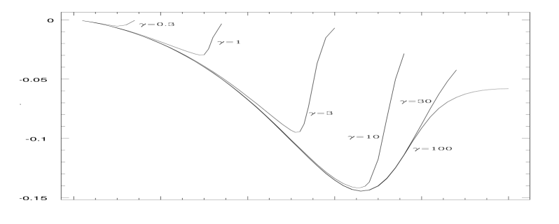
Figure 4: E vs $\tilde{\Psi}_{\rm c}$ for Wilson models.

3.3 Transition to instability

Figg. 2–4 show the plots of $E$ versus $\tilde{\Psi}_{\rm c}$ for different values of $\gamma$, for Woolley-Dickens, King end Wilson models respectively. The anisotropy parameter ranges from 100, which corresponds to nearly isotropic models, to 0.3, which corresponds to models with a strong anisotropy. The minima of these curves show the configurations in correspondence of which we have the transition between stable (to the left of the minimum) and unstable models (to the right of the minimum).

For large values of $\gamma$, only the very outer regions of the systems are affected by the presence of anisotropy and thus the equilibria are very similar to those of the corresponding isotropic systems. As expected, the critical values of $\tilde{\Psi}_{\rm c}$ tends to the critical value for isotropic systems listed in (6). As $\gamma$ decreases, the anisotropy extends deeper and deeper into the core, changing significantly the properties of the equilibria so that the critical value of the central potential is quite different from that of isotropic systems. This is clearly shown in Fig. 5 in which we have plotted the critical values of $\tilde{\Psi}_{\rm c}$ versus $\gamma$ for the models investigated. The interesting point to note is that the main effect of anisotropy is that of causing the system to become unstable at lower values of $\tilde{\Psi}_{\rm c}$.

However, we have to remark that systems with different values of $\gamma$ and the same value of $\tilde{\Psi}_{\rm c}$ do not have the same structure. This means that, although Fig. 5 gives an interesting result on the dependence of the critical value of the central potential on the amount of anisotropy in the system, it does not provide quantitative information on the issue of the change of the spatial structure of the critical model as a function of the parameter $\gamma$. In order to investigate this point, we have focussed our attention on the concentration parameter

$$c=\log\left({{r_{\rm t}}\over{r_{\rm K}}}\right),$$ (22)

and in Fig. 6 we have plotted the concentrations of the critical models, $c_{\rm crit}$, versus the parameter $\gamma$.

We see that, for King and Woolley-Dickens models, $c_{\rm crit}$ is approximately constant over a wide range of values of $\gamma$ and it starts decreasing only for $\log\gamma<0.3$, that is for systems in which the very inner regions also are significantly affected by anisotropy. This means that, for King and Woolley-Dickens models, the structure of the critical models is approximately independent on $\gamma$ and the conditions for the onset of gravothermal collapse are not significantly affected by the amount of anisotropy in the system; only for family of systems characterized by extreme anisotropy, deeply penetrating into the inner parts, the structure of the critical model changes and the instability sets in for lower values of $c$.

The situation is different for Wilson models: for these systems $c_{\rm crit}$ has a maximum for $\log\gamma\sim 0.5$ and then decreases for $\log\gamma<0.5$; in this case also, for most values of $\gamma$ investigated, the spatial structure of the critical equilibria does not vary much with the anisotropy.

Figure 5: Critical value for the onset of gravothermal instability of the dimensionless central potential versus $\gamma$ for King (dashed line), Woolley-Dickens (solid line) and Wilson (dot-dashed line) models. For any value of $\gamma$, models with $\tilde{\Psi}_{\rm c}$ larger than the critical value are unstable against gravothermal collapse.

Figure 6: Critical value (for the onset of gravothermal instability) of the concentration parameter, $c$, versus $\gamma$ for King (dashed line), Woolley-Dickens (solid line) and Wilson (dot-dashed line) models. For any value of $\gamma$, models with $c$ larger than the critical value are unstable against gravothermal collapse.

While an exact comparison with the results of numerical simulations of anisotropic systems (see the papers quoted in the Introduction) is not easy, we point out that our results are in good qualitative agreement with the results obtained by integration of the Fokker-Planck equation by Takahashi (1996) and Takahashi et al. (1997). As shown in these works, in fact, the main difference in the evolution towards core collapse of isotropic and anisotropic systems is in the evolutionary timescale, the former evolving faster than the latter. There is, instead, no significant difference in the structures of isotropic and anisotropic systems, when compared at the same evolutionary phase (see Fig. 6 in Takahashi (1995) and Fig. 2b in Takahashi et al. (1997)). As for the work of Takahashi et al. (1997), it is important to note that the maximum amount of anisotropy is reached at the moment of maximum contraction at the end of the process of core collapse and the best-fitting anisotropic King model at that phase has $\gamma=300$. We point out that our critical models refer to the structure of the systems at an earlier phase than that of maximum contraction (our critical models are meant to describe the system just at the moment of onset of gravothermal instability), when the value of $\gamma$ in the simulations of Takahashi et al. must be even larger. This means that the onset of gravothermal instability in the simulations of Takahashi et al. occurs well in the regime of high values of $\gamma$, where our analysis shows that no difference is expected between the spatial structure of the critical models for the isotropic and anisotropic case.

Additional simulations of systems with a stronger anisotropy at the moment of the onset of core collapse would be extremely interesting in order to test our conclusions about the decrease of the critical value of $c$ for small values of $\gamma$.

4 Conclusions

Models based on energy truncated distribution functions are still a very useful tool to explore some of the properties exhibited by stellar systems when they are in an enviroment that can heavily influence their characteristics: this is the case of globular clusters, but can be of relevance even in the case of elliptical galaxies in rich clusters.

In this paper, after having described their main structural properties, we have investigated, by the method of linear series, the stability against gravothermal collapse of models described by King, Wilson and Woolley-Dickens anisotropic distribution functions. The amount of anisotropy of a system has been quantified simply by means of the ratio, $\gamma=r_{\rm a}/r_{\rm K}$, of the anisotropy radius $r_{\rm a}$, which is the radius beyond which radial orbits dominate, and the King core radius $r_{\rm K}$.

We have shown that, as $\gamma$ decreases (more anisotropic systems), the central potential of the critical model decreases. The spatial structure of the critical model, globally described by the concentration parameter $c=\log(r_{\rm t}/r_{\rm K})$, remains unchanged for a wide range of values of $\gamma$ (this is true in particular for King and Woolley-Dickens models, while the range is smaller for Wilson models); in fact the concentration of the critical models as a function of $\gamma$ is approximately constant and equal to the typical value for isotropic systems down to $\log\gamma>0.3$ ($\log\gamma>1$ for Wilson models). Only for very anisotropic systems, with $\log\gamma<0.3$, the concentration of the critical models decreases as $\gamma$ decreases and the anisotropy reaches the very central regions of the systems.

We have shown that our conclusion for high values of $\gamma$ is consistent with the results of a recent investigation carried out by means of the integration of the Fokker-Planck equation for anisotropic systems by Takahashi et al. (1997), showing that no significant difference exist between the spatial structure of isotropic and anisotropic systems when they are compared at the same evolutionary phase.

We point out again that numerical simulations designed to follow the evolution of systems characterized by a stronger anisotropy at the moment of the onset of core collapse would be suitable to verify our conclusions concerning the decrease of the critical concentration for smaller values of $\gamma$.

ACKNOWLEDGEMENTS
MM acknowledges support from the Isaac Newton Scholarship.

References

Antonov V. A., 1962, Vest. Leningr. Univ., 7, 135
Bettwieser E., Spurzem R., 1986, A,A, 161, 102
Binney J., Tremaine S., 1987, Galactic Dynamics, Princeton University Press
Chernoff D., Kochanek C., Shapiro S. L., 1986, ApJ, 309, 183
Cohn H., 1980, ApJ, 242, 765
Giersz M., Heggie D. C., 1994a, MNRAS, 268, 257
Giersz M., Heggie D. C., 1994b, MNRAS, 270, 298
Giersz M., Heggie D. C., 1996, MNRAS, 279, 1037
Giersz M., Heggie D. C., 1997, MNRAS, 286, 709
Giersz M., Spurzem R., 1994, MNRAS, 269, 241
Jeans J.H., 1928, Astronomy and Cosmogony, Cambridge University Press
Katz J., 1978, MNRAS, 183, 765
Katz J., 1980, MNRAS, 190, 497
King I. R., 1965, AJ, 70, 376
Lagoute C., Longaretti P. Y., 1996, AA, 308, 441
Louis P. D., Spurzem R., 1991, MNRAS, 251, 408
Lynden-Bell D., 1967, MNRAS, 136, 101
Lynden-Bell D., Wood R., 1968, MNRAS, 138, 495
Merritt D., Tremaine S., Johnstone D., 1989, MNRAS, 236, 829
Poincaré H., 1885, Acta Math., 7, 259
Spurzem R., 1991, MNRAS, 252, 177
Spurzem R., Takahashi K., 1995, MNRAS, 272, 772
Spurzem R., Aarseth S.J., 1996, MNRAS, 282, 19
Stiavelli M., Bertin G., 1985, MNRAS, 217, 735
Takahashi K., 1995, PASJ, 47, 561
Takahashi K., 1996, PASJ, 48, 691
Takahashi K., Lee H.M., Inagaki S., 1997, MNRAS, 292, 331
Tremaine S. D., 1986, in Structure and Dynamics of Elliptical Galaxies, IAU Symp. 127, T. de Zeeuw ed.
Wilson C.P., 1975, AJ, 80, 175
Wiyanto P., Kato S., Inagaki S., 1985, PASJ, 37, 715
Woolley R., Dickens R. J., 1961, Royal Greenwich Obs. Bulletin, N. 42
Woolley R., Robertson D. A., 1956, MNRAS, 116, 288