Identification and photometry of globular clusters in M31 and M33 galaxies

Abstract

We have used the data from the DIRECT project to search for new globular cluster candidates in the M31 and M33 galaxies. We have found 67 new objects in M31 and 35 in M33 and confirmed 38 and 16 previously discovered ones. A $VI$ and $BVI$ photometry has been obtained for all the clusters in M31 and M33 respectively. Luminosity functions have been constructed for the clusters in each galaxy and compared with that of the Milky Way.

1 Introduction

Many globular cluster searches have been conducted in the M31 galaxy. The first search, conducted by Hubble (1932), resulted in the discovery of 140 globular clusters with $m_{pg}\leq 18$ mag. The first major compilation of all the globular clusters known at the time and their equatorial coordinates was compiled by Vetešnik (1962) and contained about 300 objects. Since then that number has grown to 1028 objects appearing in at least one catalogue (Fusi Pecci et al. 1993), of which only $\sim 200$ are included in the three latest major catalogues (Sargent et al. 1977, Crampton et al. 1985, Battistini et al. 1980, 1987, 1993). Most of the previous searches had been conducted on photographic plates using the technique of visual identification of potential globular clusters. The catalogues are fairly complete down to $V\sim 18$ ($M_{V}\sim 6.5$), although the degree of completeness is not uniform. According to Fusi Pecci (1993) the catalogues are incomplete:

1. in the central part of the galaxy;

2. for bright, concentrated clusters, especially if superimposed on a strong galaxy background;

3. for fainter objects.

M33 had been searched for globular clusters rather sporadically. The existence of globular clusters in that galaxy had been first noted by Sandage in 1956 (Carnegie Institution Yearbook). The only recent catalogue was compiled by Christian & Schommer (1982), containing around 200 objects.

Taking the above facts into consideration it seemed reasonable to assume that new globular clusters could be found in both galaxies, using the data collected by the DIRECT project (Kaluzny et al. 1998; Stanek et al. 1998). The frames obtained as part of that project seemed suitable for the purpose of identification and photometry of globular clusters for the following reasons:

1. large scale of the CCD frames (0.32 arcsec/pixel);

2. the limiting magnitude of the frames $V\sim 22$, in the light of completeness of the M31 catalogues down to $V\sim 18$;

3. the frames covered central regions of the galaxies, where there could still be undiscovered objects.

2 Data reduction

All the observational data used here was taken from the DIRECT project (Kaluzny et al. 1998; Stanek et al. 1998). Some additional data generated by that project was also used, as will be later noted. The frames for M31 were taken with the 1.3 McGraw-Hill telescope at Michigan-Dartmouth-MIT (MDM) Observatory using the front-illuminated, Loral $2048^{2}$ pixel CCD ”Wilbur”. At the f/7.5 station it had a pixel scale of 0.32 arcsec/pixel and a field of view of about $11^{\prime}\!\times\!11^{\prime}$. Kitt Peak Johnson-Cousins $VI$ filters were used. The observations for M33 were done with the 1.2 m telescope at the F. L. Whipple Observatory (FLWO) using a thinned, back-side illuminated, AR-coated Loral $2048^{2}$ pixel CCD “AndyCam”. The pixel scale is the same as in the case of M31. Standard Johnson-Cousins $BVI$ filters were used. The preliminary reduction of the frames was done as part of the DIRECT project and will not be discussed here. Details on that procedure can be found in Kaluzny et al. 1998. Bad columns were masked out using the IMREPLACE routine of the IRAF package.

For each of the fields in M31 ten frames were selected in $VI$ filters with sub-arcsecond seeing. Exceptions were made for field C in the $V$ filter, where only seven frames were chosen, and for field D in the $I$ filter, where only one frame was available.

The frame with the best seeing and lowest background was chosen as the template for each of the fields. The choice of the template frames was taken from the DIRECT project, as were the data used in creating lists containing the positions of common stars on the frames. The individual, non-template frames were transformed to the template coordinate system with the GEOMAP and GEOTRAN routines of the IRAF package. The frames were then averaged together using IMCOMBINE.

In the case of M33 single frames were used because of the substantial amount of bad columns on the detector. Since each frame was offset by a couple of pixels from the template, bad columns would cover a large area on the combined image, thus hindering the identification of new globular cluster candidates.

Photometry was extracted using the Daophot/Allstar package (Stetson 1987). A point spread function (PSF) varying quadratically with the position on the frame was used for the fields in M31. The PSF was modeled with a Moffat function. Stars were identified using the FIND subroutine and aperture photometry was done on them with the PHOT subroutine. Around 100 bright isolated stars were chosen for the construction of the PSF. The same stars were used as in the DIRECT project, with the exception of the M31D field in $I$ filter.

For the fields in M33 the PSF was approximated by a Moffat function linearly varying with position on the frame. Only about 50 stars were used to construct the PSF and that proved to be sufficient.

The construction of the PSF consisted of two separate stages:

1. Using a modified version of the PSF-subroutine a preliminary PSF was constructed in an iterative process. In each iteration the PSF stars with profile errors greater than twice the average were removed from the list.

2. The neighbors of the PSF stars were fitted using Allstar and then subtracted with the SUBSTAR subroutine. An improved PSF was constructed from the subtracted frame. This procedure was repeated twice.

The PSF obtained using the above method was then used by Allstar in profile photometry. In case there were stars remaining on the subtracted frame, FIND was ran again to identify them. PHOT was used to determine the aperture photometry for the newly found stars. The output file was combined with the one containing the stars found previously and used as input to Allstar. In the case of fields A, B in M33 it was found necessary to introduce another step, where stars less than 3 pixels apart were removed and Allstar was ran again on that file. The reason for this was that the second FIND had been ran with a rather low threshold. Such a procedure was used to make sure that the residuals of previously subtracted stars wouldn’t be identified and then fitted as separate objects.

3 Photometric and astrometric calibration

For all fields in M31 and fields A, B in M33 the photometric calibration from the DIRECT project was used. The transformation to the standard system was derived from observations of the Landolt fields (Landolt 1992). More details on that subject can be found in Kaluzny et al. (1998).

In the field M33C the same calibration was used as for the field B. This was possible because those fields overlapped by a substantial amount and enough bright and isolated common stars could be found in each filter.

Sample color-magnitude diagrams are shown in Figs. 1 - 3.

Figure 1: The $V/V-I$ color-magnitude diagram for the stars in field C in M31

Figure 2: The $V/V-I$ color-magnitude diagram for the stars in field C in M33

Figure 3: The $V/B-V$ color-magnitude diagram for the stars in field C in M33

The equatorial coordinates of globular clusters in M31 were derived from the data generated by the DIRECT project. In the M33 galaxy the right ascension and declination of the objects was found using reference stars from the USNO A-1 astrometric catalogue. In both cases the accuracy of the positions is better than 2 arcsec.

4 Identification and photometry of GC candidates

The following catalogues were used to identify the already known globular clusters in M31: Battistini et al. (1987); Crampton et al. (1985); Sargent et al. (1977). All objects from those catalogues which were located within the studied fields had photometry done on them, regardless whether they appeared to be globular clusters or not.

In the case of M33 the only catalogue used for this purpose was the one compiled by Christian & Schommer (1982). Magnitudes were measured only for those objects which were identified independently in this work.

The basic idea behind the identification of new globular cluster candidates was the fact that the point spread function of a globular cluster is different from that of a star. The PSF of a globular cluster should have a larger FWHM than a stellar one. Taking that into account it was expected that on the subtracted frames such objects should exhibit toroidal residuals, thus enabling their identification. Objects displaying this characteristic were selected and then their nature was verified on the original frames. The following criteria were used to discern globular clusters from other objects:

1. FWHM of the object had to be larger than that of a separate star;

2. the object had to be spherical.

Objects which didn’t meet those criteria in all filters were rejected. Remaining objects were classified on a scale from A to D,

• – very high probability globular cluster candidates, exhibiting spherical structure and a substantially larger FWHM than for a nearby star.

• – high probability globular cluster candidates. Objects in this category usually exhibited small departures from spherical shape not associated with the object itself, caused by nearby faint stars, brightness fluctuations of the galaxy background, etc.

• – objects that might be globular clusters. Such objects were usually faint and roughly spherical. Due to their faintness their radial profiles showed substantial background variations. Thus it was hard to discern whether they were globular clusters or blended stars.

• – objects that are probably not globular clusters. Objects in this category met the above criteria rather poorly, usually because of low S/N ratio. Objects from other catalogues which were found unlikely to be globular clusters were also put into this category.

It should be noted that the criteria used in the selection of globular cluster candidates were not very keen in discerning globular clusters from other non-stellar objects, especially if faint. HII regions, planetary nebulae are some of the possible sources of false identifications.

This classification is similar to the one used in the Battistini (1987) catalogue. One important difference is that for objects in classes A and B Battistini put on an additional restriction on their color.

After having created the list containing all globular cluster candidates photometry was done on them. This procedure consisted of several separate steps:

1. Selection of reference stars
   Several (3-5) reference stars were selected for each frame in order to convert the instrumental magnitudes of globular clusters to the standard system. For this purpose bright stars with known standard magnitudes were selected, located in regions with low background brightness.

2. Subtraction of neighboring stars
   Most of the globular clusters were rather faint, so it was necessary to subtract nearby stars in order not to overestimate their brightness.

3. Photometry of globular clusters
   Since the point spread function of a globular cluster differs substantially from the stellar PSF derived by Daophot and later used by Allstar, profile photometry wasn’t suitable for this purpose. Aperture photometry was used instead. Magnitudes were measured inside an aperture of 18 pixels using the PHOT subroutine. PHOT had problems determining the magnitude when there were bad pixels near a cluster, resulting from the subtraction of nearby faint objects. In such cases those pixels were filled with the value of the median computed in a box of $11\!\times\!11$ pixels. Bad columns were treated in a similar fashion. Magnitudes of objects, which incorporated the use of this method are marked in the tables by a colon.

4. Transformation to the standard system
   The standard magnitudes were determined by the following formula:

   $$M_{gc}=\frac{1}{N}\sum_{i=1}^{N}(m_{gc}-m_{ref}+M_{ref})$$ (1)

   where $m_{gc}$ and $m_{ref}$ are the instrumental magnitudes of a globular cluster and a reference star respectively, and $M_{gc}$ and $M_{ref}$ are their magnitudes referred to the standard system. N is the number of reference stars.

Magnitudes obtained in the following manner were compared with results from other catalogues. The degree of consistency was found to be satisfactory. A more detailed comparison will be presented in section 5.

The photometric data for the globular cluster candidates, along with their equatorial coordinates and finding charts are available through anonymous ftp on cfa-ftp.harvard.edu, in pub/kstanek/DIRECT directory.

5 Conclusions

5.1 Accuracy of the photometry

Our final result was the identification of new globular cluster candidates in the M31 and M33 galaxies, the confirmation of the previously discovered ones and the determination of their magnitudes, using aperture photometry, in $VI$ and $BVI$ bands, respectively.

In crowded fields the aperture photometry is less accurate than the profile photometry. As was mentioned earlier, the latter method of determining the magnitudes could not be used because the globular clusters could not be properly fitted with a stellar point spread function.

In order to estimate the errors of the magnitudes found using profile photometry a comparison was made between objects found in more than one field. The magnitudes of already discovered clusters, determined here, were compared with values taken from other catalogues.

5.1.1 Comparison within the catalogue

Taking advantage of the fact that there was some overlap between subsequent fields the magnitudes of clusters caught on two frames were compared. Such a comparison was to provide information on random errors associated with the implemented procedure of determining magnitudes. The results of the comparison are shown graphically in Figure 4.

Figure 4: A comparison of $V$ and $I$ magnitudes for objects in M31 and M33 found in two fields

The $V$ magnitudes are self-consistent to a sufficient degree over a wide range. The differences between the $I$ magnitudes of the same objects show a growing tendency with decreasing magnitude. A possible explanation of this phenomenon is that for each field different star finding thresholds were used. Thus the number of stars subtracted from the regions surrounding those objects was not the same in each case. A closer look at two such objects, 39 and 50 in the M31, revealed that the magnitudes measured in field B were lower than the values obtained for field C and, as expected, more stars were subtracted from frame B than frame C (23 stars in field B against 17 in field C for the first object and 15 versus 10 for the second). This effect was much weaker in the $V$ band since there were far less objects near the resolution limit visible in those frames. In any case the $I$ magnitudes below 17th mag should be treated with reserve.

The measurement errors were estimated at $\sigma(B)=0.05,\sigma(V)=0.9,\sigma(I)=0.18$. These values were obtained by finding the average difference between the globular cluster magnitudes measured on different frames.

5.1.2 Comparison with other catalogues

Magnitudes for the 38 already known globular clusters within the M31 fields were taken from the two following sources: Battistini 1987 ($V_{B}$); Crampton et al. 1985 ($V_{C}$). In the M33 16 previously discovered objects were identified as globular clusters, and the magnitudes of some of those objects were found in Christian & Schommer 1982 ($V_{CS1}$) and Christian & Schommer 1988 ($V_{CS2}$). The results of the comparison are showed in Figure 5.

Figure 5: A comparison of our $V$ magnitudes with data from other sources

The magnitudes of globular clusters in the M31 measured here showed good consistency with the values determined by others. The above comparison gave no indication for the existence of meaningful systematic errors in our measurements.

In the case of M33 there were relatively few objects available for comparison. Taking that into consideration and the fact that both measurements were conducted by the same persons, probably using the same method, no definite conclusions can be drawn from the comparison. The magnitudes of the brighter objects are consistent with our values. For the fainter objects there seems to be a tendency for our magnitudes to be lower than those of Christian & Schommer. Another striking feature is that the three objects appearing only in the second diagram have magnitudes that differ by $\sim 0.5-1$ mag. from our values. Taking into consideration the results of a similar comparison in M31 it seems plausible to assume that the errors of our measurements contribute a smaller amount to those large differences.

5.2 Luminosity functions

In order to obtain a qualitative comparison of the objects found in M31 and M33 with the globular cluster system of the Milky Way, luminosity functions were constructed for each of those galaxies.

Data on 143 Milky Way clusters was taken from Harris 1996. The following distance moduli were used: $\mu_{0,M31}=24.47$ mag (Stanek & Garnavich 1998), $\mu_{0,M33}=24.63$ mag (Madore & Freeman 1991). Only the clusters visible in our fields are included in the histograms for M31 and M33. It should be noted that those fields cover only parts of the galaxies, so the sample is not complete. Extinction hasn’t been accounted for. Three histograms were drawn for the M31 and M33 clusters containing: a) all of the cluster candidates found in our fields; b) A, B and C class clusters; c) A and B class clusters.

The luminosity functions are shown in Figs 6 and 7.

Figure 6: A comparison of the luminosity functions in the Milky Way and M31

Figure 7: A comparison of the luminosity functions in the Milky Way and M33

The maximum of the luminosity function of the observed M31 disk globular clusters appears to be shifted by about 2 magnitudes towards lower brightness in comparison with the Milky Way. A comparison of the halo globular cluster luminosity functions for the M31 and the Milky Way shows that the difference between their turnover magnitudes is $\sim 0.3$ mag (Harris 1993), with the M31 clusters being brighter. According to Gnedin & Ostriker (1997) the influence of dynamical effects on the cluster population is greater in the inner parts of the galaxy. In particular the destruction mechanisms are stronger in the central part. Their research indicates that low mass (hence less luminous) clusters would have short lifetimes. In accordance with the latter Gnedin (1997) found that the peak of the inner globular cluster luminosity function is brighter by 0.8 mag than for the outer clusters. Our luminosity function, constructed for the previously discovered clusters and the new globular cluster candidates, does not exhibit such behavior. Strong extinction due to the large tilt of the galaxy could be a possible, although not very likely, explanation. More research should be done in order to clarify this situation. Higher resolution observational data should be obtained for the newly discovered objects, most of them classified as C or D, in order to verify their true nature. Not much can be said about the shape of the luminosity function for A and B class clusters in M31 due to the possibility of large statistical fluctuations within such a small sample of objects. In particular the maximum of that luminosity function is shifted with respect to the other two. Another noteworthy feature is the brightness cutoff at $V\sim-10$ mag. seen in both the M31 and the Milky Way.

The luminosity function of the globulars in M33 has a maximum at the same brightness as is observed in our Galaxy. M33 is seen face on and the extinction is much weaker than in the case of M31.

5.3 Color-magnitude diagrams

The color-magnitude diagrams for the globular clusters are shown in Figs 8 - 12. Objects belonging to different classes are marked with different symbols. Class A and B clusters are denoted by circles ($\circ$), class C by boxes ($\Box$) and class D by crosses ($\times$). The stars shown in the background come from fields M31A and M33C. The photometric data for the Milky Way globulars was taken from Harris (1996).

The color-magnitude diagrams for the Milky Way’s globular clusters exhibit sharp color cutoffs at $V-I\sim 0.8$ and $B-V\sim 0.6$, with all of the clusters being located to the right of those lines.

In the $V/V-I$ diagram for M31 there is a sharp cutoff at $V-I\sim 1$ for objects brighter than $\sim 17$ mag, a value very similar to the one observed for the Milky Way’s globulars. A situation like that is not seen for fainter objects. This may result from the lower accuracy of $I$ magnitude values below 17 mag, as was mentioned in section 4.

The color-magnitude diagrams for M33 show color cutoffs at $V-I\sim 0-0.2$ and $B-V\sim 0.1$. The globular clusters in the M33 are, on the average, bluer than their Milky Way counterparts. In the $V/V-I$ diagram a B class object (A13) is seen far to the left of the region occupied by other globulars. The faintness of the object in the $I$ band (18.54 mag.) is a probable cause of the error in the $V-I$ color.

Figure 8: The $V/V-I$ color-magnitude diagram for the Milky Way globular clusters

Figure 9: The $V/B-V$ color-magnitude diagram for the Milky Way globular clusters.

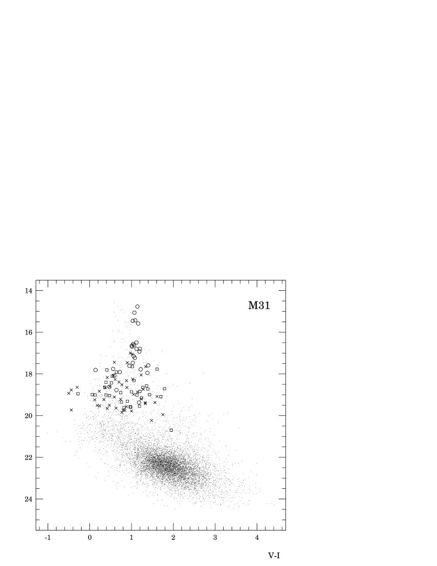
Figure 10: The $V/V-I$ color-magnitude diagram for the M31 globular cluster candidates. Class A and B clusters are denoted by circles ($\circ$), class C by boxes ($\Box$) and class D by crosses ($\times$).

Figure 11: The $V/V-I$ color-magnitude diagram for the M33 globular cluster candidates. Class A and B clusters are denoted by circles ($\circ$), class C by boxes ($\Box$) and class D by crosses ($\times$).

Figure 12: The $V/B-V$ color-magnitude diagram for the M33 globular cluster candidates. Class A and B clusters are denoted by circles ($\circ$), class C by boxes ($\Box$) and class D by crosses ($\times$).

5.4 The color-color diagram

The $V-I/B-V$ diagram for the globular clusters in the Milky Way and the M33 is shown in Fig. 13. The M33 globulars are shown as open circles and the ones in the Milky Way by triangles. Data for the Milky Way was taken from Harris (1996).

On the $V-I/B-V$ plane the Milky Way globular clusters are located in a nearly straight line extending approximately between the points $(0.8,0.6)$ and $(2.5,2.1)$. In the case of M33 the clusters also appear to form a roughly straight line of a similar slope, shifted towards lower color values.

Figure 13: The $V-I/B-V$ color-color diagram for the Milky Way and M33

5.5 A double globular cluster candidate

An object that could possibly be a double globular cluster was found in field A in the M31 galaxy. Both components were assigned a C class because of the difficulty in estimating the degree of contribution of the other object to the widening of the radial profile. The magnitudes were determined separately for each of the components by masking out the other with a value of the median computed in a box of 101 pixels on a side.

Table 1: Globular cluster candidates in the M31 galaxy
Description:
G – Sargent et al. 1977
Bo – Battistini et al. 1987
Vet – Vetesnik 1962
DAO – Crampton et al. 1985
c – object class on a scale from A to D (see p. D for more details)
f – the field in which the object is located

ID	RA (2000)	DEC (2000)	V	I	V-I	c	f	G	Bo	Vet	DAO
1	0:43:45.08	41:18:12.2	19.38	18.05	1.33	D	D
2	0:43:49.07	41:14:15.6	18.32	17.44	0.88	D	D
3	0:43:54.23	41:14:11.6	18.77	19.21	-0.44	D	D
4	0:43:57.71	41:13:52.5	17.44	16.85	0.59	D	D
5	0:43:57.96	41:21:33.2	19.73	20.17	-0.44	D	C
6	0:43:58.20	41:24:38.5	15.43	14.34	1.09	A	C	G256	Bo205	V102
7	0:43:58.64	41:30:17.9	15.06	14.00	1.07	A	C	G257	Bo206	V106
8	0:44: 0.02	41:23:11.6	17.78	16.56	1.22	A	C	G259	Bo208	V276
9	0:44: 0.81	41:17:12.5	17.95	16.57	1.38	A	D
10	0:44: 2.59	41:25:26.5	16.64	15.63	1.01	A	C	G261	Bo209	V284
11	0:44: 2.71	41:14:24.5	17.81	17.40	0.41	C	D		Bo210
12	0:44: 2.81	41:21:40.2	18.77	18.13	0.64	B	C
13	0:44: 2.83	41:20: 4.3	16.65	15.65	1.00	A	C	G262	Bo211	V98
			16.69	15.68	1.01	A	D	G262	Bo211	V98
14	0:44: 3.47	41:30:38.7	16.92	15.73	1.19	A	C	G264	Bo213	V292
15	0:44: 3.94	41:26:18.5	17.61	16.65	0.95	A	C	G265	Bo214	V286
16	0:44: 8.02	41:23:54.2	19.37	17.81	1.56	D	C
17	0:44:10.62	41:23:50.9	16.49	15.37	1.12	A	C	G269	Bo217	V281
18	0:44:11.22	41:25:22.2	17.59	16.19	1.40	B	C			V285
19	0:44:11.66	41:23:53.8	18.62	18.15:	0.47:	B	C
20	0:44:13.90	41:22:18.7	18.93	19.43	-0.50	D	C
21	0:44:14.26	41:19:19.6	14.77	13.64	1.14	A	D	G272	Bo218	V101
22	0:44:16.87	41:14:15.9	18.74	17.46	1.28	D	D		Bo277
23	0:44:18.86	41:21: 9.8	18.65	17.75	0.89	D	D
			18.64	17.92	0.72	D	C
24	0:44:19.34	41:30:35.3	16.62	15.55	1.06	B	C	G275	Bo220	V114
25	0:44:19.64	41:24: 8.5	18.64	18.93	-0.30	D	C
26	0:44:20.22	41:27:20.0	20.23	18.75	1.48	D	C
27	0:44:21.16	41:19: 9.9	18.65	17.38	1.27	C	D
28	0:44:22.05	41:33:40.1	18.66	18.29	0.37	D	B
29	0:44:23.05	41:33: 6.4	16.80	15.68	1.12	A	B	G276	Bo221	V117
30	0:44:23.32	41:35: 4.1	18.83	18.60	0.23	D	B		Bo278
31	0:44:24.28	41:33:58.5	18.90	18.15	0.74	C	B
32	0:44:25.33	41:14:11.9	17.65:	16.63	1.02:	C	D	G277	Bo222	V96
33	0:44:26.51	41:38:57.5	18.32	17.26	1.06	C	B
34	0:44:27.03	41:34:36.7	17.81	17.67	0.14	B	B	G278	Bo223
35	0:44:27.06	41:28:50.2	15.45	14.42	1.03	A	C	G279	Bo224	V112
36	0:44:27.48	41:11:34.0	17.46	16.55	0.90	D	D		Bo473
37	0:44:29.49	41:21:35.7	14.15	——	—–	A	C	G280	Bo225	V282
38	0:44:30.51	41:10:58.9	17.65	16.32	1.34	D	D		Bo226
39	0:44:31.30	41:30: 4.6	18.93	19.70	-0.77	C	B
			18.95	19.23	-0.28	C	C
40	0:44:31.49	41:27:55.2	19.59	18.61	0.98	C	C
41	0:44:33.89	41:38:28.1	16.56	15.53	1.04	A	B	G282	Bo229	V120
42	0:44:33.90	41:21: 3.2	18.64	18.27	0.36	C	C
43	0:44:34.29	41:23:11.6	19.64	19.01:	0.63:	D	C
44	0:44:34.43	41:24: 9.3	19.24	19.12	0.12	D	C
45	0:44:36.39	41:35:32.9	18.73	17.34	1.39	C	B
46	0:44:36.64	41:27:13.7	19.01	17.88	1.13	C	C
47	0:44:37.85	41:28:52.1	18.84	17.64	1.20	C	C

Table 2: Globular cluster candidates in the M31 galaxy (continued)

ID	RA(2000)	DEC(2000)	V	I	V-I	c	f	G	Bo	Vet	DAO
48	0:44:38.60	41:27:47.4	17.23	16.15	1.08	A	C	G286	Bo231
49	0:44:39.70	41:24:28.2	18.26	17.65	0.61	D	C
50	0:44:40.59	41:30: 6.0	18.60:	18.12:	0.48:	D	C
			18.82:	18.50	0.32:	D	B
51	0:44:46.37	41:29:17.7	16.80	15.60	1.20	A	C	G290	Bo234	V297
52	0:44:56.15	41:41:35.7	19.74	18.93	0.80	D	A
53	0:44:57.22	41:48: 2.3	19.09	17.39	1.70	C	A
54	0:44:59.13	41:42:25.2	19.55	18.36	1.19	C	A
55	0:44:59.61	41:33:39.3	18.99	17.56	1.43	C	B
56	0:45: 1.54	41:39: 4.4	19.58	18.61	0.97	C	A
57	0:45: 2.73	41:47: 2.5	19.95	18.20	1.75	D	A
58	0:45: 3.31	41:40: 5.6	18.55	16.86	1.68	C	A
			18.71	16.92	1.79	C	B
59	0:45: 4.03	41:46:20.7	18.43	17.92	0.52	C	A
60	0:45: 6.81	41:38:57.7	19.23	18.89	0.34	D	A
61	0:45: 7.18	41:40:31.4	18.25	17.22	1.03	D	A		Bo476		D74
62	0:45: 7.61	41:45:31.0	19.22	18.48	0.74	D	A
63	0:45: 8.30	41:39:38.0	18.17	17.75	0.42	D	B		Bo477
64	0:45: 8.31	41:39:38.0	18.07	17.50	0.57	D	A		Bo477		D75
65	0:45: 9.89	41:42:22.9	19.01	18.88	0.13	C	A
66	0:45:10.94	41:40:23.0	17.00	16.04	0.97	D	B		Bo260
67	0:45:10.96	41:40:23.0	17.05	16.03	1.02	D	A		Bo260
68	0:45:10.97	41:38:56.3	19.75	18.91:	0.84:	D	A
69	0:45:11.27	41:49:20.3	19.20	17.97	1.23	D	A
70	0:45:11.72	41:40:20.1	19.08	17.47	1.61	D	A
71	0:45:13.75	41:42:34.2	19.53	19.29	0.24	D	A
72	0:45:13.81	41:42:26.1	18.40	18.01	0.39	C	A
73	0:45:15.13	41:47:32.2	19.37	18.18	1.18	A	A
74	0:45:15.60	41:35:17.4	17.15	16.10	1.05	A	B		Bo239
75	0:45:15.80	41:44:49.6	20.70	18.76	1.95	C	A
76	0:45:16.07	41:43:22.2	18.99	18.93	0.06	C	A
77	0:45:17.37	41:39:32.9	19.51:	19.34	0.18:	D	A
78	0:45:17.72	41:41:52.6	19.50	19.03	0.47	D	A
79	0:45:17.74	41:40:58.0	19.01	18.61	0.39	C	A
80	0:45:19.57	41:48:30.3	18.52	17.74:	0.77:	D	A
81	0:45:22.26	41:47:57.1	19.78	18.78	1.00	D	A
82	0:45:26.23	41:45:52.3	19.04	18.57	0.47	C	A
83	0:45:26.94	41:45:43.5	19.11	18.52:	0.59:	D	A
84	0:45:27.15	41:43:45.2	17.76	17.20:	0.56:	B	A	G303	Bo371	V122
85	0:45:27.97	41:42: 4.1	19.57	18.70	0.88	D	A
86	0:45:28.44	41:49:29.1	18.11	17.57	0.54	C	A
87	0:45:31.98	41:49:32.2	18.05	16.81	1.23	D	A
88	0:45:32.47	41:43:33.8	19.31:	18.41:	0.90:	C	A
89	0:45:32.53	41:43:31.3	18.57:	17.22:	1.36:	C	A
90	0:45:32.94	41:48:22.8	19.85	19.08	0.77	D	A
91	0:45:33.12	41:42:19.8	18.86	17.87	1.00	C	A
92	0:45:35.60	41:45:18.4	18.98	17.92:	1.05:	D	A
93	0:45:37.44	41:40:11.2	19.35	18.59	0.76	C	A
94	0:45:39.74	41:46:34.6	19.61	18.78	0.82	C	A
95	0:45:39.82	41:44:41.8	19.15	17.91	1.24	C	A
96	0:45:41.89	41:45:33.5	15.58	14.41	1.16	A	A	G305	Bo373	V125
97	0:45:44.12	41:40: 5.6	17.77:	16.16	1.61:	C	A		Bo268		D82
98	0:45:44.54	41:41:54.6	18.08	17.49:	0.59:	A	A	G306	Bo374
99	0:45:45.58	41:45:52.9	17.91	17.20:	0.72:	B	A		Bo480	V127
100	0:45:45.58	41:39:42.5	17.47	16.44:	1.03:	A	A	G307	Bo375
101	0:45:46.25	41:48:20.3	19.42	18.09	1.33	D	A
102	0:45:46.75	41:45:22.7	19.66	19.24:	0.42:	D	A
103	0:45:48.44	41:42:40.0	17.91	17.27:	0.64:	C	A	G309	Bo376	V124
104	0:45:48.82	41:48:19.9	18.39	17.68:	0.70:	D	A
105	0:45:49.66	41:39:25.9	18.87	17.73:	1.14:	D	A

Table 3: Globular cluster candidates in the M33 galaxy
Description:
C&S – Christian & Schommer 1982
c – object class on a scale from A to D (see p. D for more details)
f – the field in which the object is located

ID	RA (2000)	DEC (2000)	B	V	I	B-V	V-I	c	f	C&S
1	1:32:56.11	30:38:25.42	17.60	17.54	17.02	0.06	0.52	A	C
2	1:33: 6.43	30:37:35.55	22.19	19.69	17.77	2.50	1.92	C	C
3	1:33:20.42	30:40:23.33	17.29	17.08	16.40	0.22	0.68	A	C
4	1:33:23.12	30:33: 0.70	17.54	17.29	17.02	0.25	0.27	A	C	H32
5	1:33:25.64	30:29:56.98	19.07	18.34	17.02	0.73	1.32	A	C
6	1:33:26.01	30:36:24.23	18.04	17.78	17.10	0.26	0.68	B	C
7	1:33:27.99	30:32:43.23	18.53	18.36	18.04	0.17	0.32	A	C
8	1:33:29.51	30:30: 2.17	18.25:	18.07:	17.53:	0.18:	0.54:	A	C
9	1:33:31.01	30:36:52.47	18.41	18.34	17.06	0.07	1.27	A	C
10	1:33:37.02	30:37:12.01	18.51:	18.49:	18.49:	0.03:	0.00:	B	C
11	1:33:37.27	30:34:14.01	17.11:	17.06	16.78:	0.05:	0.28:	A	C	U111
	1:33:37.27	30:34:14.24	17.18	16.97:	16.57:	0.21:	0.40:	B	B	U111
12	1:33:38.02	30:38: 2.17	18.06	17.40	16.29	0.66	1.11	B	C
	1:33:38.09	30:38: 3.49	18.10:	17.43	16.34	0.68:	1.09	C	B
13	1:33:38.05	30:33: 5.49	17.89:	17.62:	17.35:	0.27:	0.27:	C	B
14	1:33:39.66	30:31: 8.97	16.48	16.35	16.50	0.14	-0.16	B	B
15	1:33:40.05	30:38:27.62	16.08	15.81:	15.03:	0.28:	0.77:	B	B
16	1:33:40.40	30:43:57.68	17.22	17.11	16.65	0.11	0.46	B	A
17	1:33:41.61	30:41:42.81	17.34	16.99	16.07	0.35	0.92	D	A
18	1:33:42.99	30:42:52.60	17.13:	17.07:	17.27	0.05:	-0.20:	C	A
19	1:33:43.86	30:32:10.32	17.55	17.75	17.63	-0.21	0.13	C	B
20	1:33:44.61	30:37:53.62	17.30	17.43	18.60	-0.12	-1.18	C	B	U94
21	1:33:45.06	30:47:46.73	16.82	16.04	14.99	0.78	1.05	A	A	U49
22	1:33:52.14	30:29: 3.63	18.06	17.26	16.18	0.81	1.07	B	B	H38
23	1:33:54.15	30:33: 9.67	17.16	17.18	16.80	-0.03	0.38	C	B
24	1:33:55.18	30:47:57.88	16.81	16.53	16.19	0.29	0.34	B	A
25	1:33:57.89	30:35:31.89	18.65:	18.21:	17.75:	0.44:	0.46:	C	B
26	1:33:58.05	30:45:44.93	17.32:	17.05:	17.14:	0.26:	-0.08:	C	A	H14
27	1:34: 0.29	30:37:47.57	16.66	16.05	15.42	0.61	0.63	B	B
28	1:34: 1.61	30:42:30.72	18.01	17.88	18.54	0.13	-0.65	B	A	U75
29	1:34: 2.03	30:39:37.35	17.06	16.23	15.29	0.82	0.94	A	A
30	1:34: 2.49	30:38:40.98	17.11	17.05	17.39	0.06	-0.33	D	A
31	1:34: 2.51	30:40:40.30	17.44	16.49	15.10	0.95	1.40	A	A
32	1:34: 2.83	30:46:36.57	17.85	17.59	16.95	0.27	0.64	D	A
33	1:34: 2.94	30:43:20.60	17.02	16.31	15.31	0.71	1.00	A	A
34	1:34: 4.35	30:39:22.28	17.95	17.88	17.37	0.07	0.51	D	A
35	1:34: 7.22	30:35:23.09	17.96	17.98	18.01	-0.01	-0.03	C	B
36	1:34: 8.06	30:38:37.75	17.22	16.32	15.16	0.90	1.16	A	A
	1:34: 8.10	30:38:38.61	17.32	16.42	15.30	0.90	1.12	A	B
37	1:34: 8.55	30:39: 1.96	16.25	16.17	16.02	0.08	0.16	A	A
	1:34: 8.59	30:39: 2.87	16.35	16.34	16.14	0.01	0.20	A	B
38	1:34: 9.00	30:36:33.92	17.93:	17.76:	17.94:	0.17:	-0.18:	C	B	H30
39	1:34:10.13	30:45:29.20	17.65	17.39	17.49	0.26	-0.10	D	A	U62
40	1:34:10.69	30:45:48.70	16.07	15.98	15.71	0.09	0.27	B	A
41	1:34:10.98	30:40:29.75	18.25	17.82	17.33	0.43	0.49	B	A	U83
42	1:34:11.40	30:41:27.83	18.57	18.16	17.37	0.41	0.79	C	A	U78
43	1:34:11.57	30:34:52.43	16.81	16.52	15.96	0.29	0.57	A	B
44	1:34:14.20	30:39:58.10	18.38	17.90	17.34	0.48	0.56	D	A	U82
45	1:34:14.66	30:32:35.05	18.39:	18.07:	17.59:	0.32:	0.49:	C	B	H33
46	1:34:15.09	30:41:19.08	17.73	17.49	17.17	0.24	0.33	C	A	U79
47	1:34:18.69	30:31:37.67	16.90	16.66	16.46	0.25	0.20	B	B
48	1:34:19.47	30:46:21.15	16.92	16.69	16.20	0.23	0.49	B	A
49	1:34:19.89	30:36:12.68	17.30	17.08	16.81	0.23	0.26	A	B
50	1:34:20.21	30:39:33.13	18.91	18.61	18.13	0.30	0.48	B	A	U91
51	1:34:25.43	30:41:28.48	18.01:	17.37:	16.72:	0.64:	0.65:	B	A	H21

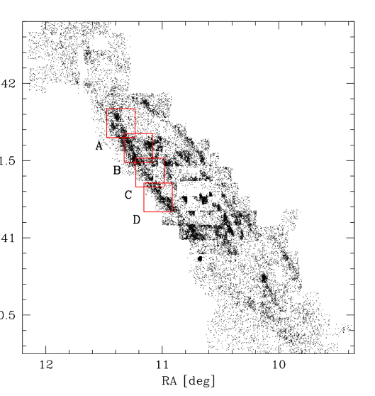
Figure 14: The location of fields A - D in the M31 galaxy

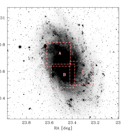
Figure 15: The location of fields A - C in the M33 galaxy

References

- (1) Battistini, P.L., Bonoli, F., Casavecchia, M., Ciotti, L., Federici, L., Fusi-Pecci, F., 1993, A&A, 272, 77
- (2) Battistini, P., Bonoli, F., Braccesi, A. Federici, L., Fusi Pecci, F., Marano, B., Borngen, F., 1987, A&AS, 67, 447
- (3) Battistini, P., Bonoli, F., Braccesi, A., Federici, L., Fusi Pecci, F., Malagnini, M.L., Marano, B., 1980, A&AS, 42, 357
- (4) Christian,C.A., Schommer, R.A., 1982, ApJS, 49, 405
- (5) Christian,C.A., Schommer, R.A., 1988, AJ, 95, 704
- (6) Crampton, D., Schade, D.J., Chayer, P., Cowley, A.P., 1985, ApJ, 288, 494
- (7) Fusi Pecci, F., Cacciari, C., Federici, L., Pasquali, A., 1993, ASP Conference Series, Vol. 48, p. 410
- (8) Gnedin, O.Y., Ostriker, J.P., 1997, ApJ, 474, 223
- (9) Gnedin, O.Y., 1997, ApJ, 487, 663
- (10) Harris, W.E., 1996, AJ, 112, 1487
- (11) Harris, W.E., 1993, ASP Conference Series, vol. 48, p. 472
- (12) Hubble, E., 1932, ApJ, 76, 44
- (13) Kaluzny, J., Stanek, K. Z., Krockenberger, M., Sasselov, D. D., Tonry, J.L., & Mateo, M., 1998, AJ, 115, 1016
- (14) Landolt, A., 1992, AJ, 104, 340
- (15) Madore, B.F., Freeman, W.L., 1991, PASP, 103, 933
- (16) Monet, D., et al., 1996, USNO-A1.0, (U.S. Naval Observatory, Washington DC)
- (17) Sargent, W.L.W., Kowal, S.T., Hartwick, F.D.A., van den Bergh, S., 1977, AJ, 82, 947
- (18) Stanek, K.Z., Garnavich, P.M., 1998, ApJ, in press (astro-ph/9802121)
- (19) Stanek, K.Z., Kaluzny, J., Krockenberger, M., Sasselov, D.D., Tonry, J.L., & Mateo, M., 1998, AJ, 115, 1894
- (20) Stetson, P.B., 1987, PASP, 99, 191
- (21) Vetešnik, M., 1962, BAC, v. 13, no. 5, p. 182