Stellar Gas Flows Into A Dark Cluster Potential At The Galactic Center

Abstract

The evidence for the presence of a concentration of dark matter at the Galactic center is now very compelling. There is no question that the stellar and gas kinematics within $\approx 0.01$ pc is dominated by under-luminous matter in the form of either a massive black hole, a highly condensed distribution of stellar remnants, or a more exotic source of gravity. The unique, compact radio source Sgr A* appears to be coincident with the center of this region, but its size (less than about $3\times 10^{14}$ cm at $\lambda$1.35 cm) is still significantly smaller than the current limiting volume enclosing this mass. Sgr A* may be the black hole, if the dark matter distribution is point-like. If not, we are left with a puzzle regarding its nature, and a question of why this source should be so unique and lie only at the Galactic center. In this paper, we examine an alternative to the black hole paradigm—that the gravitating matter is a condensed cluster of stellar remnants—and study the properties of the Galactic center wind flowing through this region. Some of this gas is trapped in the cluster potential, and we study in detail whether this hot, magnetized gas is in the proper physical state to produce Sgr A*’s spectrum. We find that at least for the Galactic center environment, the temperature of the trapped gas never attains the value required for significant GHz emission. In addition, continuum (mostly bremsstrahlung) emission at higher frequencies is below the current measurements and upper limits for this source. We conclude that the cluster potential is too shallow for the trapped Galactic center wind to account for Sgr A*’s spectrum, which instead appears to be produced only within an environment that has a steep-gradient potential like that generated by a black hole.

Submitted to the Editor of the Astrophysical Journal

1 Introduction

The Galactic center (GC) has long been suspected of harboring a central mass concentration whose gravitational influence may be the cause of the high-velocity ionized gas streamers emitting in the 12 $\mu$m [Ne II] line (Wollman (1976); Lacy, et al. (1979); for a recent review, see Mezger, Duschl & Zylka (1996)). This ionized gas appears to be in orbit about a mass distribution $\sim 3\times 10^{6}\;M_{\odot}$ within a few arcseconds (1${}^{\prime\prime}\approx 0.04$ pc at the GC) of the compact radio source Sgr A* (Lo & Claussen (1983); Serabyn & Lacy (1985)). A more recent mapping of the H92$\alpha$ line emission from Sgr A West with an angular resolution of $\sim 1^{\prime\prime}$ shows the presence of three dominant kinematic features, known as the Western Arc, the Northern Arm, and the Bar (Roberts & Goss (1993)). The former appears to be in circular rotation about Sgr A* at a radius of $\sim 1$ pc. Its velocity of $\sim 105$ km s^-1 implies that the enclosed mass is $\sim 3.5\times 10^{6}\;M_{\odot}$. Complementary studies of the $\lambda 2.17\;\mu$m Br$\gamma$ line emission from this region (Herbst, et al. (1993)) yield a mass of $\sim 5\;M_{\odot}$ for the Northern arm and the central Bar, whose dynamics require a central concentration of $\sim 4\times 10^{6}\;M_{\odot}$ within a radius of $\sim 0.17$ pc.

These early mass determinations have been supported by subsequent measurements of the stellar velocities and velocity dispersions at various distances from Sgr A*. Following the initial work by Sellgren et al. (1987), and Rieke & Rieke (1988), Haller et al. (1996) used the velocity dispersions of stars at $\gtrsim 0.1$ pc from Sgr A* to derive a compact mass of $\sim 2\times 10^{6}\;M_{\odot}$. This is consistent with the value of $\sim 2.5-3.2\times 10^{6}\;M_{\odot}$ derived by Genzel et al. (1996), using the radial velocities and velocity dispersions of $\sim 25$ early-type stars and of $\sim 200$ red giants and supergiants within the central 2 pc. A third technique for tracing the central gravitational potential is based on the acquisition of proper motions for the $\sim 50$ brightest stars within the radial range $\sim 0.004-0.4$ pc (Eckart & Genzel (1996)). These stellar motions also seem to require a central dark mass of $2-3\times 10^{6}\;M_{\odot}$, in good agreement with both the ionized gas kinematics and the velocity dispersion measurements.

Of course, showing that the GC must contain a centralized mass concentration does not necessarily imply that this dark matter is in the form of a compact object with a few million solar masses. It does not even imply that the unusual radio source Sgr A* must be associated with it. However, it is possible to demonstrate that Sgr A* is probably not stellar-like. This is based on the fact that a heavy object in dynamical equilibrium with the surrounding stellar cluster will move slowly, so that a failure to detect proper motion in Sgr A* may be used to provide an independent estimate of its mass. Using VLBI, Backer (1994) derived a lower mass limit of $\sim 20-2000\;M_{\odot}$, which appears to rule out the possibility that Sgr A* is a pulsar, a stellar binary, or a similarly small object (see also Reid et al. 1997).

Still, VLBA images of Sgr A* with milliarcsecond resolution (Lo, et al. (1993)) show that at $\lambda$1.35 cm, its size is $2.4\pm 0.2$ mas, or roughly $2.9\times 10^{14}$ cm, much smaller than the present limiting region within which the $2-3\times 10^{6}\;M_{\odot}$ are contained. So the dark matter may be distributed, perhaps in the form of white dwarfs, neutron stars, or $\sim 10\;M_{\odot}$ black holes (e.g., Haller et al. 1996). However, the latest stellar kinematic results appear to rule out the first two possible constituents. Genzel et al. (1996) argue that a distribution of neutron stars in equilibrium with the central gravitational potential should have a core radius somewhere between $0.15$ and $0.3$ pc, significantly larger than the value of $\leq 0.07$ pc derived from the velocity data. The same holds true for a population of white dwarfs. Moreover, the neutron stars would presumably have been formed with a substantial “kick” and would likely not remain bound to the nucleus (e.g., Haller, et al. (1996)). Thus, as long as the dark matter distribution is in equilibrium, and we ignore the dynamical effects of core collapse, the only viable alternative to the massive black hole paradigm may be a distributed population of $\sim 10\;M_{\odot}$ black holes. Although these objects will have formed over a Hubble time within a much larger volume, some cluster evolution calculations (Lee (1995)) have demonstrated that due to the large mass ratio of the stellar black holes to that of the normal stars, a core collapse could have driven the central component of the former to very high densities. Whether or not such a concentration is stable against mergers that would eventually produce a single massive object is still an open question.

Whatever the composition of a distributed mass concentration is, one would then be left with the task of accounting for the nature of Sgr A* itself, without the benefit of invoking the deep gravitational potential well of a point-like object (Melia (1994)). In this paper, we study in detail the emission characteristics that would be exhibited by a hot, magnetized plasma “trapped” within the dark cluster potential. In addition to the large scale gaseous features described above, there is ample observational evidence in this region for the existence of rather strong winds in and around Sgr A* itself. The key constituents of this morphology appear to be the cluster of mass-losing, blue, luminous stars comprising the IRS 16 assemblage, which is located within several arcseconds from Sgr A*. Measurements of high outflow velocities associated with IR sources in Sgr A West (Krabbe, et al. (1991)) and in IRS 16 (Geballe, et al. (1991)), the $H_{2}$ emission in the circumnuclear disk (CND) from molecular gas being shocked by a nuclear mass outflow (Gatley, I., et al. (1986)), broad Br$\alpha$, Br$\gamma$ and He I emission lines from the vicinity of IRS 16 (Hall, Kleinmann & Scoville (1982); Allen, Hyland & Hillier (1990); Geballe, et al. (1991)), and radio continuum observations of IRS 7 (Yusef-Zadeh & Melia (1991)), provide clear evidence of a hypersonic wind, with a velocity $v_{w}\sim 500-1000$ km s^-1, a number density $n_{w}\sim 10^{3-4}$ cm^-3, and a total mass loss rate $\dot{M}_{w}\sim 3-4\times 10^{-3}\;\dot{M}_{\odot}$, pervading the inner parsec of the Galaxy. If the dark matter is distributed, it is likely that a portion of this wind is captured by the compact cluster and that it settles within its potential well. Although such a configuration would not include the steep gradients associated with a black hole’s gravitational field, this trapped gas (if hot and magnetized) might conceivably still account for at least some of Sgr A*’s radiative characteristics. It is this possibility that we study here.

In § 2 of this paper, we begin with a simple hydrostatic model of the gas bound to a compact dark cluster, whose mass and size are chosen to comply with the observed stellar kinematics. Our subsequent 3-dimensional simulations of the gas flow through this mass distribution are described in § 3, and the results are presented in §4. We provide an overview of our analysis and the implications for the nature of Sgr A* in §5.

2 A Simple Hydrostatic Model Of The Gas Bound To The Dark Cluster

Before embarking on a full 3-dimensional hydrodynamical simulation of the gas flow through the dark cluster potential, let us briefly set up a simple hydrostatic model to examine the physical conditions expected for the captured plasma. For simplicity, we adopt a King model potential for the dark cluster. Later, for the hydrodynamical simulations, we will use an $\eta$-model, described below. The central mass density of the cluster is

$$\rho_{*}={9\over 4\pi u_{K}}{M_{cluster}\over r_{K}^{3}}\;,$$ (1)

where $u_{K}$ is a number of order unity that depends on how condensed the stellar distribution is, and $r_{K}$ is the King scale radius. If the tidal radius $r_{t}$ is $2r_{K}$, then $u_{K}=0.74141$. In this simple toy model, we place $10^{6}\;M_{\odot}$ of stars within $1$ core radius, corresponding roughly to $0^{\prime\prime}.02$ in projected angular size. This constitutes a linear core size $r_{K}=170$ AU’s and thus $r_{t}=340$ AU’s. The total integrated mass of this cluster is then $1.22\times 10^{6}\;M_{\odot}$, which gives $\rho_{*}=1.43\times 10^{-7}$ g cm^-3.

The gravitational potential per unit mass, measured relative to the center of the cluster, is

$$U^{\prime}={2\pi\over 3}G\rho_{*}r^{2}\;.$$ (2)

For the gas (with density $\rho$) to be in hydrostatic equilibrium within this potential, its pressure must scale according to

$${dP\over dr}=-\rho{dU^{\prime}\over dr}\;,$$ (3)

where we assume an ideal equation of state (i.e., $P_{g}=R_{g}\rho T/\mu$) and take the total pressure to be $P_{g}$ plus that of the equipartition magnetic field. Here, $R_{g}$ is the gas constant and $\mu$ is the mean molecular weight.

It is straightforward to integrate Equation (3) for a power-law temperature distribution,

$$T=T_{0}\left({r\over r_{0}}\right)^{\alpha}\;,$$ (4)

which gives

$$P=P_{0}\exp\left\{-\left({r\over\bar{r}}\right)^{2-\alpha}\right\}\;,$$ (5)

where

$$\bar{r}\equiv\left\{{2-\alpha\over 2}\,{r_{s}^{2}\over r_{0}^{\alpha}}\right\}^{1/(2-\alpha)}\;,$$ (6)

and the pressure scale height is

$$r_{s}\equiv\sqrt{{6R_{g}T_{0}\over 2\pi\mu G\rho_{*}}}\;.$$ (7)

For the gas to be confined within the core of the cluster, we must have

$$r_{s}=\eta r_{K}\;,$$ (8)

where $\eta$ is of order one. This places an upper limit on the temperature, since clearly a hotter gas will have a greater extension. More specifically, we see from Equation (7) that

$$T_{0}={2\pi\mu G\rho_{*}\eta^{2}\over 6R_{g}}\;.$$ (9)

For example, when $\alpha=-1$, we see that $T_{0}=5\times 10^{8}\eta^{2}$ K. In principle, the gas can therefore attain the temperature ($\simeq 5\times 10^{9}$ K) required to produce the observed GHz (thermal) synchrotron radiation from Sgr A* if $\eta\simeq 3$ (see Melia 1994). In addition, we see that for a captured gas mass $M_{gas}\sim 10^{-3}\;M_{\odot}$, the equipartition magnetic field can reach an intensity of $\sim 10$ gauss, or greater. This is low compared with the value ($\sim$ hundreds of gauss) used in the best fits by Melia (1994) and Narayan, Yi, and Mahadevan (1995), but is certainly within the range where an attempt to fit the spectrum with this configuration of trapped gas is interesting.

Thus, the physical conditions in this environment (i.e., the density, temperature and magnetic field) are close to the range required for the gas to emit cyclotron/synchrotron radiation at GHz wavelengths. A potential problem, however, is that the dark cluster potential is shallow inside the core, which makes the state variables depend only weakly on $r$, unlike the steep gradients that are apparently required by a spectral fit with a superposition of many thermal synchrotron components. Nonetheless, the fact that the gas is not in hydrostatic equilibrium may introduce steeper gradients due to its dynamic structure, and so definitive conclusions regarding the viability of this model to produce the GHz spectrum of Sgr A* must be based on more detailed hydrodynamic simulations, which we describe next.

3 The Physical Setup

In the absence of any outflow, many of Sgr A*’s radiative characteristics should be due to the deposition of the energy in the Galactic center wind into the central well. In the classical Bondi-Hoyle (BH) scenario (Bondi & Hoyle (1944)), the mass accretion rate for a uniform hypersonic flow past a centralized mass is

$$\dot{M}_{BH}=\pi{R_{A}}^{2}m_{H}n_{w}v_{w}\;,$$ (10)

where $R_{A}\equiv 2GM/{v_{w}}^{2}$ is the accretion radius and $M$ is the gravitating mass. At the Galactic center, for the conditions described in the Introduction, we would therefore expect an accretion rate $\dot{M}_{BH}\sim 10^{21-22}{\rm\,g\,s^{-1}}$, with a capture radius $R_{A}\sim 0.01-0.02{\rm\,pc}$. Since this accretion rate is sub-Eddington for a $\sim$ one million solar mass concentration, the accreting gas is mostly unimpeded by the escaping radiation field and is thus essentially in hydrodynamic free-fall starting at $R_{A}$. Our initial numerical simulations of this process (for a point object), assuming a highly simplistic uniform flow (Ruffert & Melia (1994); Coker & Melia (1996)) have verified these expectations.

3.1 The Wind Sources

The Galactic center wind, however, is unlikely to be uniform since many stars contribute to the mass ejection. So for these calculations, we assume that the early-type stars enclosed (in projection) within the Western Arc, the Northern Arm, and the Bar produce the observed wind. Thus far, 25 such stars have been identified (Genzel, et al. (1996)), though the stellar wind characteristics of only 8 have been determined from their He I line emission (Najarro, et al. (1997); see Table 1). Two of those sources, IRS 13E1 and IRS 7W, seem to dominate the mass outflow with their high wind velocity ($\sim 1000{\rm\,km\,s^{-1}}$) and a mass loss rate of more than $2\times 10^{-4}\;M_{\odot}$ yr^-1 each. Unfortunately, the temperature of the stellar winds is not well known, and so for simplicity we have assumed that all the winds are Mach 30; this corresponds to a temperature of $10^{4-5}$K. In addition, for the sources that are used in these calculations, their location in $z$ (i.e., along the line of sight) is determined randomly with the condition that the overall distribution in this direction matches that in $x$ and $y$. With this proviso, all these early-type stars are located within the central parsec surrounding Sgr A*. For the calculations reported here, the sources are assumed to be stationary over the duration of the simulation. The stars without any observed He I line emission have been assigned a wind velocity of $750{\rm\,km\,s^{-1}}$ and an equal mass loss rate chosen such that the total mass ejected by the 14 stars used here is equal to $3\times 10^{-3}\;M_{\odot}$ yr^-1. In Figure 1, we show the positions (relative to Sgr A*) of these wind sources; the size of the circle marking each position corresponds to the relative mass loss rate (on a linear scale) for that star. Note that although we have matched the overall mass outflow rate to the observations, we have only used 14 of the 25 stars in the sample. There are two principal reasons for this: (1) stars further away than 10 arcsec (in projection) from Sgr A* are outside of our volume of solution and therefore could not be included, and (2) due to our computational resolution limits, we needed to avoid excessively large local stellar densities. So small clusters of adjacent stars were replaced with single wind sources.

3.2 The Dark Cluster Potential

Following Haller & Melia (1996), we will represent the gravitational potential of the dark cluster with an “$\eta$-model” (Tremaine, et al. (1994)). This function represents an isotropic mass distribution with a single parameter, so that the mass enclosed within radius $\tilde{r}$ (in dimensionless units) is given by

$$M_{\eta}(\tilde{r})\propto{{{\tilde{r}}^{\eta}}\over{(1+{\tilde{r}})^{\eta}}}\;.$$ (11)

We here restrict our examination to the case $\eta=2.5$ since this provides the closest approximation to a King model that is physically realizable (i.e., a nonnegative distribution function), and we scale the mass so that $2\times 10^{6}\;M_{\odot}$ are enclosed within 0.01 pc (see Fig. 2). With this, the total integrated mass of the dark cluster is $2.7\times 10^{6}\;M_{\odot}$. Thus, writing $\tilde{r}$ in units of $R_{A}$ (i.e., $r\equiv s\tilde{r}\times R_{A}$), and choosing $s$ to yield the observed enclosed mass at $0.01$ pc (see Fig. 2), we get

$$M_{\eta}(r)=2.7\times 10^{6}\left({{13.84r}\over{1+13.84r}}\right)^{5/2}\;M_{\odot}\;.$$ (12)

A more recent assessment of the enclosed mass (Genzel, et. al. (1997)) places a yet more rigorous constraint on the possibility of a distributed dark matter component. These newer observations may indeed invalidate the idea that any realistic stable distribution of small mass objects can account for the observed potential. In the future, it may be of interest to carry out a calculation similar to that reported here, but for a more condensed dark matter distribution consistent with this latest observation. As we shall see, however, the present hydrodynamical calculation strongly suggests that a cluster potential cannot easily reproduce Sgr A*’s spectrum, and this next generation of calculations may therefore be unnecessary.

In a complex flow, generated by many wind sources, the wind velocity and density are not uniform, so the accretion radius may not be independent of angle. To set the length scale for the simulations, we shall therefore adopt the value $R_{A}=.018{\rm\,pc}$ (for which 1^′′ = 2.3 $R_{A}$) as a reasonable mean representation of this quantity.

3.3 The Hydrodynamical Modeling

3.3.1 The Hydrodynamics Code

We use a modified version of the numerical algorithm ZEUS, a general purpose code for MHD fluids developed at NCSA (Stone & Norman (1992); Norman (1994)). The code uses Eulerian finite differencing with the following relevant characteristics: fully explicit in time; operator and directional splitting of the hydrodynamical variables; fully staggered grid; second-order (van Leer) upwinded, monotonic interpolation for advection; consistent advection to evolve internal energy and momenta; and explicit solution of internal energy. More details can be found in the references. The code was run on the massively parallel Cray T3E at NASA’s Goddard Space Flight Center under the High Performance Computing Challenge program. The production run for the calculation presented here used 125 T3E processors and ran at more than 8 Gflops. The code assigns each processor to a “tile” and each tile consists of $60^{3}$ zones. Zone sizes are geometrically scaled by a factor of 1.02 so that the central zones are $\sim 20$ times smaller than the outermost zones, mimicking the “multiply nested grids” arrangement used by other researchers (e.g., Ruffert & Melia (1994)). This allows for maximal resolution of the central region (within the computer memory limits available) while sufficiently resolving the wind sources and minimizing zone-to-zone boundary effects. The total volume is $(40R_{A})^{3}$ or $\sim(0.7{\rm\,pc})^{3}$ with the center of the dark cluster distribution being located at the origin.

The density of the gas initially filling the volume of solution is set to a small value and the velocity is set to zero. In order to reach equilibrium more quickly, the internal energy density is chosen such that the initial temperature is $\sim 10^{2}$ K. Free outflow conditions are imposed on the outermost zones and each time step is determined by the Courant condition with a Courant number of 0.5. The 14 stellar wind sources are modeled by forcing the velocity in 14 subregions of 125 zones each to be constant with time while the densities in these subvolumes are set so that the total mass flow into the volume of solution, $\dot{M}_{w}$, is given by Table 1. Also, the magnetic field of the winds is assumed to always be at equipartition. The angular momentum and mass accretion rates reported in the next section are calculated by summing the relevant quantity in zones located within $0.1R_{A}$ of the origin.

3.3.2 Heating and Cooling

Although we are modeling the wind sources more realistically than in previous work, we here ignore the effects of the magnetic field on the large scale kinematics. We take the medium to be an adiabatic polytropic gas, with $\gamma=5/3$. Building on previous work (Melia (1994) and Coker & Melia (1997)), we have included a first order approximation to magnetic dissipative heating as well as an accurate expression for the cooling due to magnetic bremsstrahlung, thermal bremsstrahlung, line emission, radiative recombination, and 2 photon continuum emission for a gas with cosmic abundance. For magnetic heating, we assume that the magnetic field never rises above equipartition. If compression and flux conservation would otherwise dictate a magnetic field larger than the equipartition value, the field lines are assumed to reconnect rapidly, converting the magnetic field energy into thermal energy, thereby re-establishing equipartition conditions. In the future, we will use a more detailed treatment of this dissipation process based on the scheme described in Kowalenko & Melia (1997).

The cooling function includes a multiple-Gaussian fit to the relevant cooling emissivities provided by N. Gehrels (see Gehrels & Williams (1993) and references cited therein), though with the thermal bremsstrahlung portion supplanted with more accurate expressions that are valid over a broader range of physical conditions and with the inclusion of magnetic bremsstrahlung. For the former, we use (Rybicki & Lightman (1979))

$$\epsilon_{TB}=2.84\times 10^{-27}n_{e}^{2}T^{1/2}{\rm\,erg\,s^{-1}\,cm^{-3}}\;,$$ (13)

with a Gaunt factor of 1.2 and a Z of 1.3 (Rybicki & Lightman (1979)), while for the latter (Melia (1994))

$$\epsilon_{MB}=1.06\times 10^{-15}G(T)n_{e}B^{2}{\rm\,erg\,s^{-1}\,cm^{-3}}\;,$$ (14)

where $n_{e}$ is the electron number density, $T$ is the temperature, $B$ is the magnetic field, and $G(T)$ is an analytical approximation to Equation (27) in Melia (1994) (good to better than 5%), given by the expression

$$G(T)={{3X^{2}+12X+12}\over{X^{3}+X^{2}}}\;,$$ (15)

where $X=m_{e}c^{2}/kT$. The ionization fraction, $\Delta$, is found by balancing recombination with collisional ionization (Rossi et. al. (1997)) and setting $n_{e}=\Delta n_{H}$, where $n_{H}$ is the Hydrogen number density. This involves solving Equation (1e) in Rossi et al. (1997) for $\Delta$ assuming that the left hand side is zero:

$$\Delta={{1}\over{1+0.445T^{-1}e^{157890/T}}}\;.$$ (16)

In addition, when calculating $n_{e}$, we ensure that radiative cooling ceases below $3\times 10^{3}$K; it is likely that the assumption of steady state equilibrium, made in deriving the cooling rates in Gehrels & Williams (1993), is invalid below this temperature. Figure 3 shows the resulting emissivities as functions of $T$ for a magnetic field of 10 milliGauss and a Hydrogen number density $n_{H}=10^{4}{\rm\,cm^{-3}}$. Note that cooling due to Comptonization and any pair production have not yet been included since they are not thought to be significant in the vicinity of Sgr A*. Also, it is assumed that the optical depth is small throughout the volume of solution.

3.4 Calculation of the Spectrum

In order to calculate the observed continuum spectrum, we assume that the observer is positioned along the negative $z$-axis at infinity and we sum the emission from all zones that are located at a projected distance, $R_{xy}$, of less than $0.1\,R_{A}$. Further, we assume that scattering is negligible and that the optical depth is less than unity. At the temperature and density that we encounter here, the dominant components of the continuum emissivity are electron-ion ($\epsilon_{ei}$) and electron-electron ($\epsilon_{ee}$) bremsstrahlung. Due to the interstellar medium’s weak magnetic field ($\sim\mu G$), the emissivity from magnetic bremsstrahlung, even at small $r$, is orders of magnitude smaller than $\epsilon_{ei}$ and $\epsilon_{ee}$. In the non-relativistic limit, we use $\epsilon_{ei}^{NR}$ and $\epsilon_{ee}^{NR}$ based on the expressions in Gould (1980) and Gould (1981), though excluding the Sommerfeld and other higher order corrections. Defining $E=h\nu/m_{e}c^{2}$ and $\beta=h\nu/2k_{B}T$, we have

$$\epsilon_{ei}^{NR}=C_{ei}^{NR}(1+Ef/4)e^{-\beta}k_{0}(\beta)\sqrt{X}n_{e}^{2}\;,$$ (17)

where $f=1/4\beta+k_{1}(\beta)/k_{0}(\beta)$, $k_{0}$ and $k_{1}$ are the 0th and 1st order modified Bessel functions, respectively, and $C_{ei}^{NR}$ is a constant given by

$$C_{ei}^{NR}={{4}\over{3\pi}}\sqrt{{{2}\over{\pi}}}ch\alpha^{3}(\lambda/2\pi)^{2},$$ (18)

where $\alpha$ is the fine-structure constant, $\lambda$ is the electron’s Compton wavelength, $c$ is the speed of light, and $h$ is Planck’s constant. Here, and in the following expressions, the units of $\epsilon$ are erg s^-1 Hz^-1 steradian^-1 cm^-3 Similarly, we have

$$\epsilon_{ee}^{NR}=C_{ee}^{NR}\sqrt{T}\beta e^{-\beta}k_{0}(\beta)gn_{e}^{2}\;,$$ (19)

where

$$g={{3}\over{4\beta}}+{{k_{1}(\beta)}\over{k_{0}(\beta)}}+{{0.9e^{-\beta}k_{0}(\beta)}\over{\beta}}\;,$$ (20)

and

$$C_{ee}^{NR}={{128}\over{15}}\alpha^{3}\lambda^{2}h\sqrt{{{k_{B}}\over{\pi m_{e}}}}\;.$$ (21)

For the relativistic electron-ion bremsstrahlung emissivity, we use an expression from Quigg (1968). Defining $\beta_{1}\equiv h\nu/k_{B}T$, then we have

$$\epsilon_{ei}^{ER}=C^{ER}{{k_{2}(X)}\over{X^{2}}}e^{-\beta_{1}}\left({{40}\over{3}}+{{4\beta_{1}}\over{3}}-\beta_{1}^{2}+\left({{16}\over{3}}+{{8\beta_{1}}\over{3}}+2\beta_{1}^{2}\right)\left(\log{{{2}\over{X}}}-\gamma\right)+e^{\beta_{1}}Ei(-\beta_{1})\left(-{{16}\over{3}}+{{8\beta_{1}}\over{3}}-2\beta_{1}^{2}\right)\right)n_{e}^{2}$$ (22)

where $Ei$ is the exponential integral, $k_{2}$ is the 2nd order modified Bessel function, $\gamma$ is Euler’s constant and $C^{ER}$ is a constant given by

$$C^{ER}={{r_{0}^{2}\alpha ch}\over{2\pi}}\;,$$ (23)

with $r_{0}$ the classical electron radius. For the relativistic electron-electron bremsstrahlung emissivity, we use an expression from Alexanian (1968):

$$\epsilon_{ee}^{ER}=C^{ER}e^{-\beta_{1}}\left({{28}\over{3}}+2\beta_{1}+{{\beta_{1}^{2}}\over{2}}+\left({{16}\over{3}}+{{8\beta_{1}}\over{3}}+2\beta_{1}^{2}\right)\left(\log{{{2}\over{X}}}-\gamma\right)-e^{\beta_{1}}Ei(-\beta_{1})\left({{8}\over{3}}-{{4\beta_{1}}\over{3}}+\beta_{1}^{2}\right)\right)n_{e}^{2}.$$ (24)

In the transrelativistic region ($X\sim 1$), we use a weighted average of the NR and ER expressions. Note that the above equations are slightly different from those in the references due to a number of typographical errors in the originals. Taking the effects of refraction into account, the final calculated luminosity is

$$L_{\nu}=4\pi\sum_{ij}^{R_{ij}<1R_{A}}\sum_{k}(\epsilon_{ei}+\epsilon_{ee})\sqrt{1-{{e^{2}n_{e,ijk}}\over{\pi m_{e}\nu^{2}}}}\;dV_{ijk}\;e^{-\sum_{1}^{k}d\tau_{k}}\;,$$ (25)

where $k$ is the zone number along the line of sight, $d\tau_{k}$ is its optical depth and $n_{e,ijk}$ is the electron number density within the zone $(ijk)$. Refraction is important only below $\sim 0.2$ GHz, where it accounts for the low-frequency turnover evident in the spectra shown in Figure 8.

4 Results

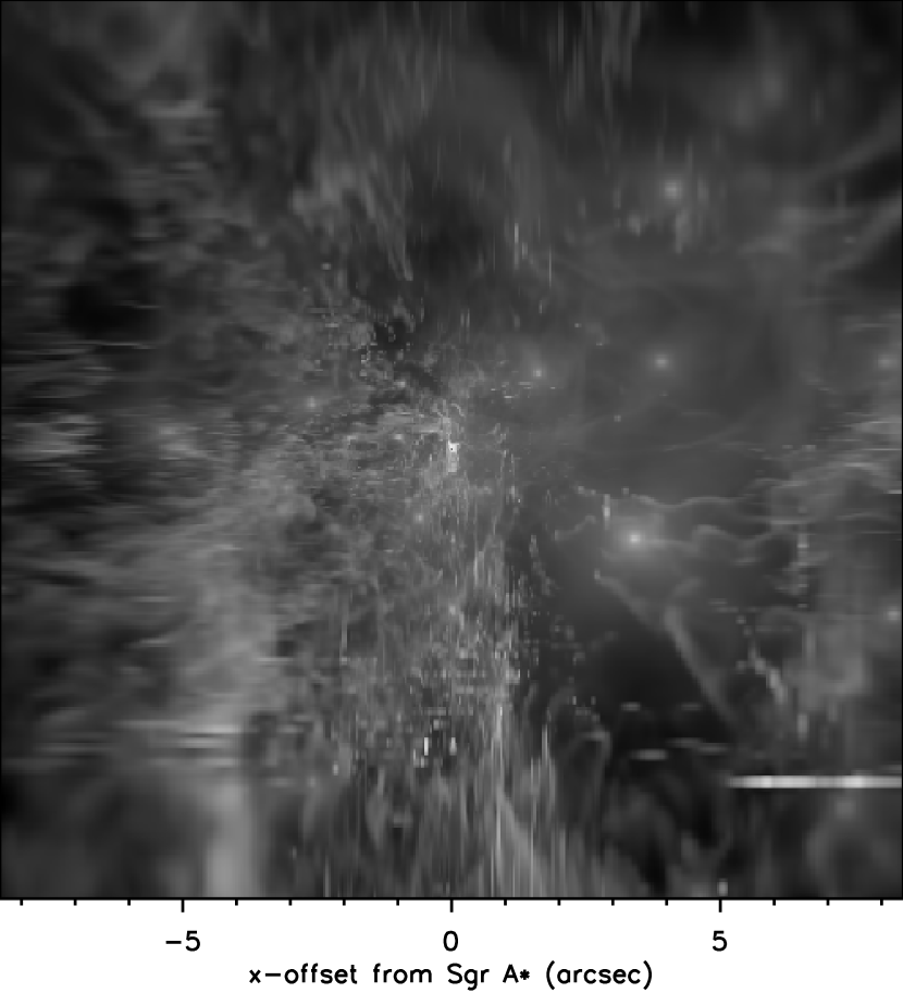
Figure 4: A plot of the line-of-sight column density along the $z$-axis for the hydrodynamical simulation at the end of the calculation (at $\sim$ 1450 years). The grey scale is logarithmic with solid white corresponding to a column density of $\sim 1.2\times 10^{21}{\rm\,cm^{-2}}$ and black corresponding to $\sim 6.5\times 10^{16}{\rm\,cm^{-2}}$. Sgr A* is located at the center of the image.

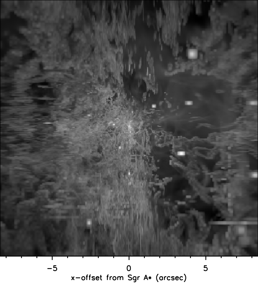
Figure 5: A plot of the line-of-sight integrated emissivity along the $z$-axis for the hydrodynamical simulation at ($\sim$ 1450 years). For this figure, it is assumed that there is no scattering or absorption. The grey scale is logarithmic with solid white corresponding to a frequency-integrated intensity of $\sim 1.1\times 10^{5}$ erg cm^-2 s^-1 steradian^-1, and black corresponding to $\sim 1\times 10^{-2}$ erg cm^-2 s^-1 steradian^-1. Sgr A* is located at the center of the image. For reference, note that the volume of this central region is $7\times 10^{47}$ cm.

The large scale gas morphology through the central dark cluster toward the end of the hydrodynamical simulation is shown in Figures 4 and 5. Figure 4 is a plot of the column density viewed along the $z$-axis while Figure 5 shows the emitted intensity (i.e., the integrated emissivity along the line-of-sight). Of particular interest in these images is the appearance of streaks of high-velocity gas (“streamers”) that are very reminiscent of features, such as the so-called “Bullet” seen near the Galactic center (Yusef-Zadeh, et al. 1996). In our simulation, these structures are produced predominantly within the wind-wind collision regions, and in the future, we shall consider in greater detail the possibility that the observed high-velocity gas components near Sgr A* are produced in this fashion. Note in these figures the relative locations of the wind-producing stars (see also Fig. 1), and the dominant role played by IRS 13E1 to the lower right of the compact radio source.

It should also be noted that the gas distribution in a multiple-wind source environment like that modeled here is distinctly different from that of a uniform flow past a central accretor (Coker & Melia 1997). Unlike the latter, the former does not produce a large-scale bow shock, and therefore the environmental impact of the gravitational focusing by the central dark mass has significantly less order in this case. For example, it is less likely in a multiple-wind source environment that the interaction between a centralized mass and the Galactic center wind can craft the type of channeled flow required to produce the mini-cavity. We shall defer a more extensive discussion of this point to a later publication in which we report the results of a multiple-wind source simulation for the case in which the dark matter is in the form of a massive black hole rather than a distributed dark cluster.

In Figure 6 we show the mass enclosed within a sphere of radius 0.1 $R_{A}$ as a function of time, centered on the midpoint of the dark cluster. In similar fashion, Figure 7 is a plot of the enclosed energy within this same volume. After reaching equilibrium several sound crossing times after the start of the simulation, the enclosed mass and energy begin to fluctuate aperiodically, reflecting the turbulent cell nature of the flow in and out of the central region. Typically $2.7\times 10^{-3}\;M_{\odot}$ of gas (the dashed line in this figure) is trapped within the cluster at any given time. Note also that although the gas is highly supersonic, with most of the energy in kinetic form, the thermal energy can be boosted rather suddenly when the enclosed magnetic field energy is dissipated. This occurs when strong shocks pass through this region; the shocks compress the field sufficiently to the point where it reaches, or even surpasses, equipartition and dissipation ensues. The turbulent, time-dependent nature of the flow is clearly evident in this Figure too.

VLBA imaging of Sgr A* (Lo, et al. 1993) restricts its size at $\lambda$1.35 cm to $2.4\pm 0.2$ mas, corresponding to a linear dimension of $\approx 2.9\times 10^{14}$ cm. The smallest cell size in our simulation is $7\times 10^{14}$ cm. To minimize the inaccuracy due to numerical fluctuations, we have calculated the spectrum from a central region roughly $10$ times this size ($0.1R_{A}$), to include at least $100$ zones. Thus clearly our predicted spectrum constitutes an upper limit to the actual emission expected from Sgr A*. We have also introduced the additional simplification of ignoring the line emission. Since the average gas temperature within these zones is $\sim 10^{7}$ K, the contribution to the luminosity due to fb and bb processes (see Fig. 3) is at most comparable to (though mostly less than) that due to continuum processes. Further, the line emission will not contribute significantly to the radio portion of the spectrum. For simplicity, we have therefore only calculated the continuum spectrum from this central region for comparison with that observed from Sgr A*.

We show the predicted spectrum for this simulation in Figure 8. Not surprisingly, the spectrum has characteristics very reminiscent of a hot gas trapped in a shallow gravitational potential (e.g., Limaneto, et al. 1997). That is, it is an accumulation of bremsstrahlung components with a high-energy shoulder characteristic of the highest temperature $T_{max}$ attained by the gas. In our simulation, $T_{max}$ never reached the values required for cyclotron/synchrotron emission to become important (see § 2 above). As such, the radio luminosity is more than 4 orders of magnitude below that actually observed from Sgr A*. This is of course consistent with the brightness temperature limit associated with this source. We note also that the flux predicted by this process at X-ray and $\gamma$-ray energies is significantly below that required to account for the ROSAT datum (Predehl & Truemper 1994) and is well below the SIGMA upper limit (Goldwurm, et al. 1994).

5 Discussion

Based on the simulation reported here, it does not appear that the gravitational potential of a cluster of stellar remnants, even an extremely compact one, can compress the gas from stellar winds to the point where the temperature, density and magnetic field are sufficient to drive an observationally significant cyclotron/synchrotron emissivity at GHz frequencies. As we speculated earlier, this is due entirely to the fact that the cluster potential is flat in its middle, unlike the steep gradients encountered by the infalling gas near a black hole. Although the spatial resolution near the origin can be improved over that used here, it is unlikely that this improvement in the model can alter this deficiency of the flattened cluster potential.

Thus, aside from the issue of (i) whether an equilibrium dark cluster can even account for the observed Galactic center potential, and (ii) whether such a compact cluster can be stable over a significant fraction of the age of the Galaxy, our 3D hydrodynamical simulation has demonstrated that the radio emissivity from the gas trapped within this cluster cannot reproduce Sgr A*’s spectrum. The alternative viable options would therefore appear to be (i) that Sgr A* is unrelated to the accreting or trapped Galactic center gas, which then raises the question of why such a unique source should lie only at the Galactic center, and (ii) that Sgr A* is the signature of an accreting, massive black hole.

Our simulation has also raised other very interesting and important questions that are best pursued elsewhere. These include the nature of the high-velocity gas streamers observed in radio continuum images of the Galactic center, and the specifics of the environmental impact of multiple wind sources interacting with the central black hole.

Acknowledgments We gratefully acknowledge helpful discussions with Joseph Haller regarding the central cluster potential. This work was partially supported by NASA grants NAGW-2518 and NGT-51637.

Table 1: Parameters for Galactic Center Wind Sources

Star	x (arcsec)	y (arcsec)	z (arcsec)	v (${\rm\,km\,s^{-1}}$)	$\dot{M}$(${10}^{-5}\;M_{\odot}$ yr-1)
IRS 16NE	-2.6	0.8	5.5	550	9.5
IRS 16NW	0.2	1.0	7.3	750	5.3
IRS 16C	-1.0	0.2	-7.1	650	10.5
IRS 16SW	-0.6	-1.3	4.9	650	15.5
IRS 13E1	3.4	-1.7	-1.5	1000	79.1
IRS 7W	4.1	4.8	-5.1	1000	20.7
AF	7.3	-6.7	8.5	700	8.7
IRS 15SW	1.5	10.1		700	16.5
IRS 15NE	-1.6	11.4		750	18.0
IRS 29N	1.6	1.4	3.5	750	12.9
IRS 33E	0.0	-3.0	1.5	750	12.9
IRS 34W	3.9	1.6	-6.4	750	12.9
IRS 1W	-5.3	0.3	7.8	750	12.9
IRS 9NW	-2.5	-6.2	-3.8	750	12.9
IRS 6W	8.1	1.6	3.6	750	12.9
AF NW	8.3	-3.1	-2.1	750	12.9
BLUM	9.2	-5.0
IRS 9S	-5.5	-9.2
Unnamed 1	1.3	-0.6
IRS 16SE	-1.4	-1.4
IRS 29NE	1.1	1.8
IRS 7SE	-2.7	3.0
Unnamed 2	3.8	-4.2
IRS 7E	-4.2	4.9
AF NWW	10.2	-2.7

Figure 1: Location of the 14 wind-producing stars used in the simulation reported below, relative to the position of Sgr A* indicated by the * symbol. The radius of each circle corresponds (on a linear scale) to that star’s mass loss rate. Setting the scale is 13E1, with $\dot{M}=7.9\times 10^{-4}\;M_{\odot}$ yr^-1.

Figure 2: Plot of the enclosed mass versus distance from Sgr A* in an $\eta$-model with $\eta=2.5$. Also shown is a recent observational determination of the enclosed mass ($2.5\pm 0.5\times 10^{6}{\,M_{\odot}}$) within 0.015 pc (Eckart & Genzel 1997).

Figure 3: A plot of emissivity versus temperature used in the simulations, for the representative parameter values $B=10^{-2}$ Gauss and $n_{H}=10^{4}$ cm^-3. The solid curve is the total, the dot-dashed curve corresponds to thermal bremsstrahlung, the dashed curve is for magnetic bremsstrahlung, and the dotted curve corresponds to the sum of the other cooling mechanisms (see text).

Figure 6: A plot of mass enclosed within 0.1 $R_{A}$ versus time for the hydrodynamical simulation. The dashed line is the average ($2.7\times 10^{-3}{\,M_{\odot}}$) value for times beyond 1000 years. Note the frequent large amplitude fluctuations over a time scale of less than a few decades.

Figure 7: Plot of energy enclosed within 0.1 $R_{A}$ versus time for the hydrodynamical simulation. The solid, dashed, and dotted curves correspond to thermal, kinetic, and magnetic energy, respectively. Note that the thermal energy rises whenever the magnetic energy is dissipated. Also, peaks in the thermal energy are often associated with rapid changes in the kinetic energy; this occurs when shock fronts travel through the central region.

Figure 8: Plot of the predicted luminosity density versus frequency for 3 points in time during the 3D hydrodynamical simulation. The solid, dotted, and dashed curves are at approximately 1200, 1300, and 1400 years, respectively, after the start of the simulation. Equilibrium occurs after several sound crossing times, corresponding roughly to 1000 years.

References

- Alexanian (1968) Alexanian, M. 1968, Phys. Rev., 165, 253.
- Allen, Hyland & Hillier (1990) Allen, D., Hyland, A., & Hillier, D. 1990, MNRAS, 244, 706.
- Backer (1994) Backer, D.C. 1994, in The nuclei of normal galaxies, ed. R. Genzel & A.I. Harris (Dordrecht: Kluwer), 403.
- Bondi & Hoyle (1944) Bondi, H, & Hoyle, F. 1944, MNRAS, 104, 273.
- Coker & Melia (1996) Coker, R., & Melia, F. 1996, in ASP Conf. Vol. 102, The Galactic Center: 4th ESO/CTIO Workshop, ed. R. Gredel (San Francisco: ASP), 403.
- Coker & Melia (1997) Coker, R. & Melia, F., 1997, ApJ (Letters), 488, L149..
- Eckart & Genzel (1997) Eckart, A., & Genzel, R. 1997, MNRAS, 284, 576.
- Eckart & Genzel (1996) Eckart, A. & Genzel, R. 1996, Nature, 383, 415.
- Gatley, I., et al. (1986) Gatley, I., Jones, T., Hyland, A., Wade, R., Geballe, T., & Krisciunas, K. 1986, MNRAS, 222, 299.
- Geballe, et al. (1991) Geballe, T., Krisciunas, K., Bailey, J., & Wade, R. 1991, ApJ (Letters), 370, L73.
- Gehrels & Williams (1993) N. Gehrels & Williams, E. D. 1993, ApJ (Letters), 418, L25.
- Genzel, et al. (1996) Genzel, R., et al. 1996, ApJ, 472, 153.
- Genzel, et. al. (1997) Genzel, R., Eckart, A., Ott, T. & Eisenhauer, F. 1997, MNRAS, 291, 219.
- Goldwurm, et al. (1994) Goldwurm, A., et al. 1994, Nature, 371, 589.
- Gould (1980) Gould, R. J. 1980, ApJ, 238, 1026.
- Gould (1981) Gould, R. J. 1981, ApJ, 243, 677.
- Hall, Kleinmann & Scoville (1982) Hall, D., Kleinmann, S., & Scoville, N. 1982, ApJ (Letters), 260, L53.
- Haller & Melia (1996) Haller, J.M., & Melia, F. 1996, ApJ, 464, 774.
- Haller, et al. (1996) Haller, J.M., et al. 1996, ApJ, 456, 194.
- Herbst, et al. (1993) Herbst, T.M., Beckwith, S.V.W., Forrest, W.J., Pipher, J.L. 1993, AJ, 105, 956
- Kowalenko & Melia (1997) Kowalenko, V. & Melia, F. 1997,Aust. J. Phys., in press.
- Krabbe, et al. (1991) Krabbe, A., Genzel, R., Drapatz, S., & Rotaciuc, V. 1991, ApJ (Letters), 382, L19.
- Lacy, et al. (1979) Lacy, J.H., Baas,F., Townes, C.H. & Geballe, T.R. 1979, ApJ, 227, 217.
- Lee (1995) Lee, H.M. 1995, MNRAS, 272, 605.
- Limaneto, et al. (1997) Limaneto, G.B., et al. 1997, A&A, 327, 81L
- Lo, et al. (1993) Lo, K.Y., et al. 1993, Nature, 362, 38.
- Lo & Claussen (1983) Lo, K.Y. & Claussen, M.J. 1983, Nature, 306, 647.
- Melia (1994) Melia, F. 1994, ApJ, 426, 577.
- Mezger, Duschl & Zylka (1996) Mezger, P.G., Duschl, W.J. & Zylka, R. 1996, A.A. Rev, 7, 289.
- Najarro, et al. (1997) Najarro, F., Krabbe, A., Genzel, R., Lutz, D., Kudritzki, R., & Hillier, D. 1997, A&A, 325, 700
- Narayan, Yi & Mahadevan (1995) Narayan, R., Yi, I. & Mahadevan, R. 1995, Nature, 374, 623.
- Norman (1994) Norman, M. 1994, BAAS, 184, 50.01
- Predehl & Truemper (1994) Predehl, P.; Truemper, J. 1994, A&A, 290L, 29P
- Quigg (1968) Quigg, C. 1968, ApJ, 151, 1187.
- Reid, et al. (1997) Reid, M.J., Readhead, A.C.S., Vermeulen, R. & Treuhaft, R. 1997, BAAS, 191, 97.06
- Rieke & Rieke (1988) Rieke, G.H. & Rieke, M.J. 1988, ApJ, 330, L33.
- Roberts & Goss (1993) Roberts, D.A. & Goss, W.M. 1993, ApJS, 86, 133
- Rossi et. al. (1997) Rossi, P., Bodo, G., Massaglia, S., & Ferrari, A. 1997, A&A, 321, 672
- Ruffert & Melia (1994) Ruffert, M., & Melia, F. 1994, A.A.Letters, 288, L29.
- Rybicki & Lightman (1979) Rybicki, G. & Lightman, A. 1979, Radiative Processes in Astrophysics (Wiley and Sons: New York).
- Sellgren et al. (1987) Sellgren, K., et al. 1987, ApJ, 317, 881.
- Serabyn & Lacy (1985) Serabyn, E. & Lacy, J.H. 1985, ApJ, 293, 445.
- Stone & Norman (1992) Stone, J.M., & Norman, M.L. 1992, ApJS, 80, 753
- Tremaine, et al. (1994) Tremaine, S., Richstone, D. O., Byun, Y., Dressler, A., Faber, S. M., Grillmair, C., Kormendy, J., & Lauer, T. R. 1994, AJ, 107, 634
- Wollman (1976) Wollman, E. 1976, Ph.D. Thesis, Univ. California, Berkeley.
- Yusef-Zadeh & Melia (1991) Yusef-Zadeh, F. & Melia, F. 1991, ApJ (Letters), 385, L41.
- Yusef-Zadeh, et al. (1996) Yusef-Zadeh, F., Roberts, D.A., Goss, W.M., Frail, D. & Green, A. 1996, ApJ (Letters), 466, L25.