Images and Spectra From the Interior of a Relativistic Fireball

Abstract

The detection of an afterglow, following a $\gamma$-ray burst (GRB), can be described reasonably well by synchrotron emission from a relativistic spherical expanding blast wave, driven by an expanding fireball. We perform detailed calculations considering the emission from the whole region behind the shock front. We use the Blandford McKee self similar adiabatic solution to describe the fluid behind the shock. Using this detailed model, we derive expressions for the peak flux, and the peak frequency at a given observed time. These expressions provide important numerical corrections to previous, more simplified models. We calculate the observed light curve and spectra for several magnetic field models. We show that both the light curve and the spectra are flat near the peak. This rules out the interpretation of the optical peak of GRB970508 as the peak of the light curve, predicted by the existing fireball models. We calculate the observed image of a GRB afterglow. The observed image is bright near the edge and dimmer at the center, thus creating a ring. The contrast between the edge and the center is larger at high frequencies and the width of the ring is smaller.

1 Introduction

The detection of delayed X-ray, optical and radio emission, “afterglow”, following a GRB is reasonably described by emission from a spherical relativistic shell, decelerating upon collision with an ambient medium (Waxman 1997a, Mészáros & Rees 1997, Katz & Piran 1997, Sari, Piran & Narayan 1998). A relativistic blast wave is formed and expands through the surrounding medium, heating the matter in it’s wake. The observed afterglow is believed to be due to synchrotron emission of relativistic electrons from the heated matter. The surrounding medium will be referred to as interstellar medium (ISM), though this may not necessarily be the case.

At any given time, a detector receives photons which were emitted at different times in the observer frame, at different distances behind the shock front and at different angles from the line of sight (LOS) to the center of the GRB. The properties of the matter are different at each of these points, and so are the emissivity and the frequency of the emitted radiation. Early calculations have considered emission from a single representative point (Mészáros & Rees 1997, Waxman 1997a, Sari, Piran & Narayan 1998). Later works included more detailed calculations. Synchrotron emission was considered from the shock front (Sari 1998, Panaitescu & Mészáros 1998), and monochromatic emission was considered from a uniform shell (Waxman 1997b).

We consider an adiabatic hydrodynamical evolution, and use the adiabatic self similar solution found by Blandford and McKee (1976) for a highly relativistic blast wave expanding into a uniform cold medium, which we will refer to as the BM solution. We neglect scattering, self absorption and electron cooling. Self absorption becomes important at frequencies much smaller than the peak frequency, and for slow cooling, electron cooling becomes important at frequencies much higher than the peak frequency, so this should yield a good approximation for the observed flux around the peak. An analysis of the spectrum over a wider range of frequencies was made by Sari, Piran and Narayan (1998).

In section 2 we derive the basic formula for the observed flux from a system moving relativistically. In section 3 we consider synchrotron emission from a power law electron distribution, and calculate the observed light curve and spectra. We show that both the light curve and the spectra are flat near the peak. This causes difficulty in explaining the shape of the optical peak of GRB970508 (Sokolov et. al. 1997). We obtain expressions for the peak frequency at a given observed time, and for the peak flux. In section 4 we consider three alternative magnetic field models. We show that the light curve and the spectra remain flat near the peak in all the cases we considered.

In section 5 we calculate the observed light curve and spectra from a locally monochromatic emission. We consider a uniform shell approximation, which was calculated by Waxman (1997c), and compare the light curve and spectra to those obtained for the BM solution. We show that a uniform shell approximation yields results which are considerably different from those obtained for a more realistic hydrodynamics, and very different from those obtained for a realistic emission together with a realistic hydrodynamics.

In section 6 we calculate the surface brightness, thus obtaining the observed image of a GRB afterglow. As indicated in previous works (Waxman 1997b), Sari 1998, Panaitescu & Mészáros 1998), we obtain from detailed calculations, that the image appears brighter near the edge and dimmer near the center, creating a ring near the outer edge. At a given observed time, the contrast between the edge and the center of the image is larger and the width of the ring is smaller at high frequencies, while at low frequencies the contrast is smaller and the width of the ring is larger.

2 The Formalism

We consider a system that is moving relativistically while emitting radiation. We obtain a formula for the flux that is measured by a distant detector (i.e. $D\gg L$ where D is the distance to the detector, and L is the size of the area emitting radiation). We use a spherical coordinate system and place the origin within the emitting region (i.e. at the source), while the z-axis points towards the detector (see Figure 1). The detector is at rest in this frame, and so is the ambient ISM. We refer to this frame as the observer frame. Consider a small volume element $dV=r^{2}drd\mu d\phi$ (where $\mu\equiv\cos\theta$) and let $j^{\prime}_{\nu^{\prime}}$ be the energy per unit time per unit volume per unit frequency per unit solid angle, emitted by the matter within this volume in it’s local frame (note that generally $j_{\nu}$ depends on the direction $\Omega$ as well as on the frequency, place and time). We denote quantities measured in the local rest frame of the matter with a prime, while quantities without a prime are measured in the observer frame. Note that $j_{\nu}/\nu^{2}$ is Lorentz invariant (Rybici & Lightman 1979) and $\nu^{\prime}=\nu\gamma(1-\beta\mu_{v})$, where $\gamma$ and $\beta c$ are the Lorentz factor and the velocity of the matter emitting the radiation, respectively, and $\mu_{v}$ is the cosine of the angle between the direction of the velocity of the matter and the direction to the detector, in the observer frame). The contribution to $I_{\nu}$ from this volume element is given by:

$$dI_{\nu}\cong j_{\nu}{dr\over\mu}={j^{\prime}_{\nu^{\prime}}\over\gamma^{2}(1-\beta\mu_{v})^{2}}{dr\over\mu}$$ (1)

(see Figure 1). The contribution to the flux at the detector is $dF_{\nu}\cong I_{\nu}d\Omega$ where $\Omega$ is the solid angle seen from the detector, and $I_{\nu}$ includes all the contributions from different volume elements along the trajectory arriving at the detector from the direction $\Omega$ simultaneously and at the time for which $F_{\nu}$ is calculated. Consider a photon emitted at time $t$ and place $\vec{\bf r}$ in the observer frame. It will reach the detector at a time $T$ given by;

$$T=t-{r\mu\over c}\ ,$$ (2)

where $T=0$ was chosen as the time of arrival at the detector of a photon emitted at the origin at $t=0$. Using $\alpha\cong r\sqrt{1-\mu^{2}}/D$, we obtain:

$$F(\nu,T)={1\over D^{2}}\int^{2\pi}_{0}d\phi\int^{1}_{-1}d\mu\int^{\infty}_{0}r^{2}dr{{j^{\prime}(\Omega^{\prime}_{d},\nu\gamma(1-\beta\mu_{v}),{\vec{\bf r}},T+{r\mu\over c})}\over\gamma^{2}(1-\beta\mu_{v})^{2}}\ ,$$ (3)

where $j^{\prime}=j^{\prime}(\Omega^{\prime},\nu^{\prime},{\vec{\bf r}},t)$, and later $P^{\prime}=P^{\prime}(\nu^{\prime},{\vec{\bf r}},t)$. $j^{\prime}$ is taken in the direction $\Omega^{\prime}_{d}$ at which a photon should be emitted in order to reach the detector, and $\gamma,\beta,\mu_{v}$ should be taken at the time $t$ implied by equation 2.

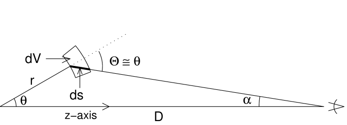
Figure 1: The contribution of a volume element $dV$ to the flux observed by a distant observer is $dF_{\nu}\approx I_{\nu}d\Omega$, where $I_{\nu}=j_{\nu}ds$. Since the observer is far away, the direction of emission in the observer frame is almost parallel to the z-axis.

For a spherical expanding system, which emits isotropically in it’s local rest frame, one obtains $\mu_{v}=\mu$ and $j^{\prime}_{\nu}=P^{\prime}_{\nu}/4\pi$, so that:

$$F(\nu,T)={1\over 2D^{2}}\int^{1}_{-1}d\mu\int^{\infty}_{0}r^{2}dr{{P^{\prime}(\nu\gamma(1-\beta\mu),r,T+{r\mu\over c})}\over\gamma^{2}(1-\beta\mu)^{2}}\ .$$ (4)

Note that because of relativistic effects, a jet with an opening angle $\theta>1/\gamma$ around the LOS can be considered locally as spherical (Piran 1994).

In order to learn whether the radial integration is important, we calculate the observed flux from emission only along the LOS. We do this by considering a situation in which at each point the photons are emitted only radially: $j^{\prime}_{\nu^{\prime}}=P^{\prime}_{\nu^{\prime}}\delta(\Omega^{\prime}-\Omega^{\prime}(\hat{r}))$. Note that the correct limit is obtained when the delta function in the direction of the emission is taken in the local frame. Since $d\Omega=\gamma^{2}(1-\beta\mu)^{2}d\Omega^{\prime}$ (Rybici & Lightman 1979) we obtain that:

$$\delta(\Omega^{\prime}-\Omega^{\prime}(\hat{r}))=\gamma^{2}(1-\beta\mu)^{2}\delta(\Omega-\Omega(\hat{r}))\ .$$ (5)

Substituting this $j^{\prime}$ in equation 3 we obtain:

$$F(\nu,T)={1\over D^{2}}\int^{\infty}_{0}r^{2}dr{P^{\prime}({\nu\over\gamma(1+\beta)},r,T+{r\over c})}\ .$$ (6)

Equation 4 is quite general, and includes integration over all space. In the case of GRB afterglow, radiation is emitted only from the region behind the shock front. The spacial integration should therefore be taken over a finite volume, confined by the surface of the shock front. We would therefore like to obtain an explicit expression for the radius of the shock $R$ as a function of $\mu\equiv\cos\theta$ for a given arrival time $T$. In the case of a shell moving with a constant velocity $\beta c$, one obtains from equation 2:

$$R={\beta cT\over 1-\beta\mu}\ .$$ (7)

If one considers a constant arrival time $T$, this equation describes an ellipsoid, which confines the volume constituting the locus of points from which photons reach the detector simultaneously (Rees 1966). In GRBs, most of the matter is concentrated in a thin shell which decelerates upon collision with the ambient medium. When the deceleration of the shell is accounted for, the ellipsoid is distorted. The details of this distortion depend on the evolution of the shock radius $R(t)$ (Sari 1998, Panaitescu & Mészáros 1998). In this paper we consider an adiabatic ultra-relativistic hydrodynamic solution, which implies $\Gamma\propto R^{-3/2}$, where $\Gamma$ is the Lorentz factor of the shock. For this case, equation 2 yields:

$$R={cT\over 1-\mu+1/(8\Gamma^{2})}\ .$$ (8)

The shape of the volume constituting the locus of points from which photons reach the detector simultaneously resembles an elongated egg (see Figure 2), and will be simply referred to as the “egg”. The side facing the observer (the right side in the Figures) will be referred to as the front of the “egg”, and the side closer to the origin (the left side in the figures) will be referred to as the back of the “egg”.

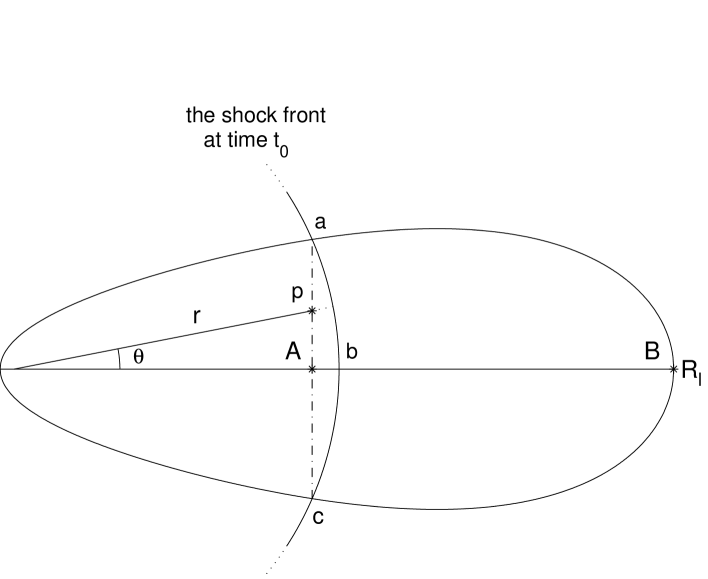
Figure 2: We see here the egg-shaped region from which photons reach an observer at a given time $T$. In all the figures of the “egg” the observer is located far to the right, and the symmetry axis is the LOS to the center of the GRB. In order to reach the observer simultaneously, photons emitted at different locations should be emitted at different times in the observer frame, according to equation 2. Photons that are emitted simultaneously in the observer frame along the dashed-dotted line $ac$, reach the observer simultaneously. Therefore $ac$ represents an equal $y$ contour line. The location of the shock front at this time of emission is indicated by the solid line $abc$, and it’s radius $R$ appears in the definitions of $y,$ and $\chi$. A photon emitted at point A, at a distance of $d=r/\gamma^{2}$ behind the shock front and at a time $t_{0}$ (both in the observer frame) caches up with the shock front at point B, at a later time $t_{1}$ in the observer frame.

From hydrodynamic considerations, we expect the typical size of the region emitting radiation behind the shock, to scale as: $\Delta\propto R/\Gamma^{2}$ in the observer frame. Despite this fact, it is still important to consider the emission from the whole volume of the “egg”, whose limits are given by equation 8. To illustrate this we give a simple example. Consider a photon emitted on the LOS at a distance $d=R/\gamma^{2}$ behind the shock (point A in Figure 2) at a time $t_{0}$ in the observer frame, where $\gamma=\Gamma/\sqrt{2}$ is the Lorentz factor of the matter just behind the shock. This Photon will catch up with the shock front at a later time $t_{1}$ in the observer frame (at point B in Figure 2), and will arrive at the detector together with a photon emitted at that point at $t_{1}$. From equation 8 we find that on the LOS: $R=16\gamma^{2}cT$, and so we obtain that $R(t_{1})/R(t_{0})=17^{1/4}\cong 2$. This shows that the emission comes from a substantial part of the volume of the “egg”, and not just from a thin layer near it’s surface. This is illustrated by the shaded region in figures 6 and 11, which corresponds to a shell of width $\Delta=R/4\gamma^{2}$ in the observer frame.

At a given observed time $T$, the emission should be considered from the volume of the “egg” whose surface is described by equation 8. Taking this into account, it is simpler to calculate the flux at a given observed time $T$, using new variables $y,\chi$ that depend on $T$ (see Figures 2 and 3):

$$y\equiv{R\over R_{l}}\ \ \ \ \ \ \ ,\ \ \ \ \ \ \ \chi\equiv 1+16\gamma_{f}^{2}\left({R-r\over R}\right)\ ,$$ (9)

where $R=R(t)$ is the radius of the shock front, $\gamma_{f}$ is the Lorentz factor of the matter just behind the shock and $R_{l}$ is the radius of the point on the shock front, on the LOS from which a photon reaches the detector at a time $T$ (see Figure 2). Since we expect the typical size of the emitting region behind the shock, to scale as: $\Delta\propto R/\gamma^{2}$, the choice of $\chi$ is natural to this problem. The exact form of $\chi$ was chosen to suit the BM solution, discussed below. Using equation 2 we can express $r,\mu$ in terms of $y,\chi$:

$$r\cong R_{l}y\ \ \ \ \ \ \ \ ,\ \ \ \ \ \ \ \ \mu\cong 1-{1-\chi y^{4}\over 16\gamma_{l}^{2}y}\ ,$$ (10)

where $\gamma_{l}$ is the Lorentz factor of the matter just behind the shock, on the LOS.

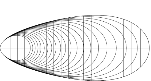
Figure 3: Equal-$y$ contour lines ($y=0.1,0.15,...,0.95$) - vertical lines, and equal-$\chi$ contour lines ($Log_{10}(\chi)=0,0.15,0.3,...,3$) - curved lines. The horizontal line is the LOS to the observer, which is located far to the right.

We would like to express equation 4 in terms of $y,\chi$. This will enable us to calculate the flux for the BM solution. This solution describes an adiabatic highly relativistic blast wave expanding into an ambient uniform and cold medium (Blandford & McKee 1976). In terms of $y$ and $\chi$ the BM solution is given by:

$$n^{\prime}=4\gamma_{f}n_{1}\chi^{-5/4}\ \ \ ,\ \ \ \gamma=\gamma_{f}\chi^{-1/2}\ \ \ ,\ \ \ e^{\prime}=4n_{1}m_{p}c^{2}\gamma_{f}^{2}\chi^{-17/12}\ ,$$ (11)

where $n^{\prime}$ and $e^{\prime}$ are the number density and the energy density in the local frame, respectively, $\gamma$ is the Lorentz factor of the bulk motion of the matter behind the shock, $m_{p}$ is the mass of a proton, $n_{1}$ is the number density of the unshocked ambient ISM in it’s local rest frame and $\gamma_{f}=\gamma_{l}y^{-3/2}$. For the BM solution, one obtains (Sari 1997):

$$\gamma_{l}\cong 3.65E_{52}^{1/8}n_{1}^{-1/8}T_{days}^{-3/8}\quad,\quad R_{l}\cong 5.53\times 10^{17}E_{52}^{1/4}n_{1}^{-1/4}T_{days}^{1/4}\rm{cm}\ ,$$ (12)

where $E_{52}$ is the total energy of the shell in units of $10^{52}\rm{erg}$, $n_{1}$ is the number density of the ISM in units of $\rm cm^{-3}$ and $T_{days}$ is the observed time in days.

For any spherically symmetric self similar solution we can define $g(\chi)$ by: $\gamma^{2}\equiv\gamma_{f}^{2}g(\chi)$, where $g(\chi)$ describes how $\gamma$ varies with the radial profile. For the BM solution $g(\chi)=\chi^{-1}$, and for a uniform shell $g(\chi)=1$. Using the definitions above, we obtain from equation 4 after the change of variables:

$$F(\nu,T)={8R_{l}^{3}\over D^{2}}\int^{\infty}_{1}d\chi\int^{\chi^{-1/4}}_{0}dy{y^{10}P^{\prime}(T,\nu\gamma(1-\beta\mu),y,\chi)\over{\left[1+y^{4}\left(8g(\chi)^{-1}-\chi\right)\right]^{2}g(\chi)}}\ .$$ (13)

This formula for the flux takes into consideration the contribution from the whole volume behind the shock front, and will be referred to as the general formula.

We would like to single out the angular integration and the radial integration, in order to find out the different effects each integration has on the observed flux.

In order to single out the effect of the angular integration we consider a thin shell of thickness $\Delta$ in the observer frame and take the limit $\Delta\to 0$. Because of kinematical spreading we expect $\Delta$ to scale as: $\Delta\propto R/\gamma^{2}$. According to the definition of $\chi$, such a shell corresponds to a constant interval in $\chi$ , i.e. the shell lies within the interval $\chi\in[1,\chi_{max}]$ for some $\chi_{max}$. The limit $\Delta\to 0$ corresponds to taking a delta function in $\chi$ : $\delta(\chi-1)$.

In order to single out the effect of the radial integration, we changed variables in equation 6 from $r$ to $\chi$. For the BM solution we obtain:

$$F(\nu,T)={R_{l}^{3}\over 4D^{2}}\int^{\infty}_{1}d\chi\chi^{-7/4}P^{\prime}(T,{\nu\over\gamma(1+\beta)},\chi)\ .$$ (14)

3 Synchrotron Emission

According to the fireball model, a highly relativistic shell moves outward and is decelerated upon collision with the ambient ISM. This creates a relativistic blast wave that expands through the ISM and heats up the matter that passes through it. The relativistic electrons of the heated material emit synchrotron radiation in the presence of a magnetic field.

We now consider the synchrotron emission at a certain point, in which the values of $n^{\prime},\gamma$ and $e^{\prime}$ are given by the hydrodynamic solution. In order to estimate the local emissivity, we assume that the energy of the electrons and of the magnetic field at each point are a fixed fraction of the total internal energy at that point: $e^{\prime}_{el}=\epsilon_{e}e^{\prime}$ , $e^{\prime}_{B}=\epsilon_{B}e^{\prime}$. We assume that the shock produces a power law electron distribution: $N(\gamma_{e})=K{\gamma_{e}}^{-p}$ for $\gamma_{e}\geq\gamma_{min}$ (for the energy of the electrons to remain finite we must have $p>2$). In the Figures for which a definite numerical value of $p$ is needed, we use $p=2.5$. The constants $K$ and $\gamma_{min}$ in the electron distribution can be calculated from the number density and energy density:

$$\gamma_{min}=\left({p-2\over p-1}\right){\epsilon_{e}e^{\prime}\over n^{\prime}m_{e}c^{2}}\ \ \ \ \ \ ,\ \ \ \ \ \ K=(p-1)n^{\prime}\gamma_{min}^{p-1}\ .$$ (15)

Assuming an isotropic velocity distribution, the total emitted power of a single average electron (i.e. with $\gamma_{e}=\langle\gamma_{e}\rangle$) is given by:

$$P^{\prime}_{e,av}={4\over 3}\sigma_{T}c\beta^{2}\langle\gamma_{e}\rangle^{2}e^{\prime}_{B}\quad,\quad\langle\gamma_{e}\rangle\equiv{\epsilon_{e}e^{\prime}\over n^{\prime}m_{e}c^{2}}$$ (16)

(Rybici & Lightman 1979), where $\sigma_{T}$ is the Thomson cross section and $e^{\prime}_{B}=B^{2}/8\pi$, where $B$ is the magnetic field (in the local frame). Although we refer to the magnetic field in the local frame, throughout the paper, we make an exception and write it without a prime.

The synchrotron emission function (power per unit frequency) of a single electron is characterized by $P_{\nu,e}\propto\nu^{1/3}$ for frequencies much smaller than the electrons synchrotron frequency, and it drops exponentially at large frequencies. The typical synchrotron frequency, averaged over an isotropic distribution of electron velocities, is given by:

$$\nu^{\prime}_{syn}(\gamma_{e})={3\gamma_{e}^{2}q_{e}B\over 16m_{e}c}\ ,$$ (17)

where $m_{e}$ and $q_{e}$ are the mass and the electric charge of the electron, respectively. We approximate the emission of a single electron as $P_{\nu,e}\propto\nu^{1/3}$ up to the electrons typical synchrotron frequency, where we place a cutoff in the emitted power. We normalized the emission function so that the total power emitted by a single electron equals that of an exact synchrotron emission.

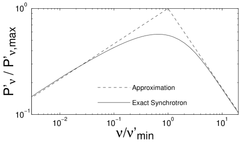
Figure 4: The local emissivity from a power law distribution of electrons, emitting synchrotron radiation. The solid curve represents exact synchrotron emission with an isotropic electron velocity distribution, while the dashed curve represents the approximation we used for the local emissivity. The differences in the local emissivity tend to smear out when integration is performed over the whole volume behind the shock front.

Under these assumptions, we obtain after integration over the power law electron distribution, that the spectral power per unit volume (in the local frame) at any given point is:

$$P^{\prime}_{\nu}=\left\{\matrix{P^{\prime}_{\nu,max}\left({\nu\over\nu^{\prime}_{min}}\right)^{1/3}&\nu<\nu^{\prime}_{min}\cr P^{\prime}_{\nu,max}\left({\nu\over\nu^{\prime}_{min}}\right)^{-{p-1\over 2}}&\nu>\nu^{\prime}_{min}}\right.\quad,$$ (18)

where $\nu^{\prime}_{min}=\nu^{\prime}_{syn}(\gamma_{min})$ is the synchrotron frequency of an electron with the minimal Lorenz factor at that point. Since the emitted power at each point peaks at $\nu^{\prime}_{min}$, this frequency can be looked upon as the typical emitted frequency around which the emitted power is concentrated. Although this emission function was obtained by approximating the spectral emission of each electron as having the shape of the low frequency tail ($\propto\nu^{1/3}$), the spectral power for the whole electron distribution resembles that obtained for an exact synchrotron emission and an isotropic electron velocity distribution. The solid curve in Figure 4 represents the local emissivity from an exact synchrotron emission of an isotropic distribution of electrons (Rybici & Lightman 1979, Wijers & Galama 1998), while the dashed curve represents equation 18 with:

$$P^{\prime}_{\nu,max}=0.88\times{4(p-1)\over(3p-1)}{n^{\prime}P^{\prime}_{e,av}\over\nu^{\prime}_{syn}(\langle\gamma_{e}\rangle)},$$ (19)

where a factor of $0.88$ was added to improve the fit to the exact synchrotron emission. In our calculations we use the local emission represented by the dashed line in Figure 4. This local emission differs from that of an exact synchrotron emission near the peak, by up to $\sim 45\%$, and is only slightly different above or below the peak. Note that differences in the local emissivity tend to get smeared out, when the contribution to the observed flux is integrated over the whole volume behind the shock front. We expect that considering exact synchrotron emission should somewhat lower the peak flux and the peak frequency, and make the light curve and spectra more rounded and flat near the peak. We evaluate that the peak flux would be lower by about $30\%$. Since there are only slight differences in high and low frequencies, there should hardly be any effect on the value of the point where the extrapolations of the power laws at high and low frequencies meet (see Table 1).

In this section we use the BM hydrodynamical solution. The combination of the realistic emission function described above, and a realistic hydrodynamical solution should yield a reasonable approximation for the observed flux.

The results are presented as a function of the dimensionless similarity variable $\phi\equiv\nu/\nu_{T}$, where $\nu_{T}$ is defined as the observed synchrotron frequency of an electron with $\gamma_{e}=\gamma_{min}$ just behind the shock on the LOS:

$$\nu_{T}\equiv\nu_{min}(y=\chi=1)=1.54\times 10^{15}\sqrt{1+z}\left({p-2\over p-1}\right)^{2}\epsilon_{B}^{1/2}\epsilon_{e}^{2}E_{52}^{1/2}T_{days}^{-3/2}\rm Hz$$ (20)

where $z$ is the cosmological red shift of the GRB. Our results can therefore be looked upon, with the proper scaling of the logarithmic x-axis, either as the spectra at a given observed time or as the light curve at a fixed observed frequency.

Similarly, we express the observed flux in terms of a “standard” flux $F_{0}$ defined by:

$$F_{0}\equiv{N(R_{l})P_{\nu,peak}\over 4\pi D^{2}}\quad,\quad P_{\nu,peak}\equiv 0.88{P_{e,av}(R_{l})\over\nu_{syn}(\gamma_{l})}=0.88{P^{\prime}_{e,av}(R_{l})\gamma_{l}\over\nu^{\prime}_{syn}(\gamma_{l})}\ ,$$ (21)

where $P^{\prime}_{e,av}(R_{l})$ and $\nu^{\prime}_{syn}(\gamma_{l})$ are the total power and synchrotron frequency of an average electron at $y=\chi=1$, respectively, $P_{\nu,peak}$ is an estimate of the peak spectral power of an average electron, and $N(R_{l})\equiv 4\pi R_{l}^{3}n_{1}/3$ is the total number of electrons behind the shock at the time $t$ in the observer frame for which $R(t)=R_{l}$. Allowing for cosmological corrections, $F_{0}$ is given by:

$$F_{0}=8.24\times 10^{4}(1+z)\epsilon_{B}^{1/2}E_{52}n_{1}^{1/2}\left({d_{L}\over 10^{28}\rm{cm}}\right)^{-2}\rm{\mu J}\ ,$$ (22)

where $d_{L}$ is the luminosity distance of the GRB.

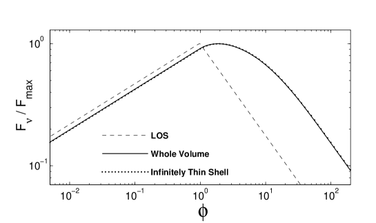
Figure 5: The observed flux from synchrotron emission of a power law electron distribution for the BM solution. The different curves stand for emission only along the LOS, emission from an infinitely thin shell, and emission from the whole volume behind the shock. The emission from the whole volume is very similar to that obtained for an infinitely thin shell, due to a coincidence that rises from our choice for the magnetic field model (see section 4).

The results for the observed flux are presented in Figure 5. The flux arriving from the LOS (the dashed curve) peaks at $\phi_{peak}\cong 0.98$, and is only slightly rounded near the peak. The flux arriving from an infinitely thin shell (the dotted curve) peaks at $\phi_{peak}\cong 1.92$ and is quite rounded and flat near the peak. The flux arriving from the whole volume behind the shock front (the solid curve) peaks at $\phi_{peak}\cong 1.88$ and is flat and rounded near the peak, quite resembling the flux from an infinitely thin shell.

Our best prediction for the flux measured by a distant detector is obtained when we assume a realistic hydrodynamical solution (the BM solution), a realistic radiation emission and use the general formula (see the solid curve in Figure 5). We would now like to examine it more closely. The curve looks quite flat near the peak, and we attempt to demonstrate this feature in a quantitative manner. If one compares the peak flux obtained by extrapolation of the power laws, obtained at low and high frequencies, to the “actual” peak flux, one obtains that it is larger by a factor of $1.53$: $F_{extr}=1.53F_{\nu,max}$. In order to further estimate the flatness of the curve near the peak, we define $\phi_{+}$ and $\phi_{-}$ by $F_{\nu}(\phi_{+})=F_{\nu}(\phi_{-})=0.5F_{\nu,max}$, where $\phi_{+}>\phi_{peak}>\phi_{-}$. We obtain that $\phi_{-}\approx 0.1\phi_{peak}$ and $\phi_{+}\approx 10\phi_{peak}$, so that $\phi_{+}/\phi_{-}\sim 100$. In a similar manner, we define $T_{+}$ and $T_{-}$ for a given observed frequency, by $F_{\nu}(T_{+})=F_{\nu}(T_{-})=0.5F_{\nu,max}$, where $T_{+}>T_{peak}>T_{-}$. One obtains: $T_{+}/T_{-}=(\phi_{+}/\phi_{-})^{2/3}\sim 20$ (note that $T_{+}$ and $T_{-}$ are frequency independent).

The frequency at which the observed flux peaks at a given observed time $T$ is given by:

$$\nu_{peak}=\phi_{peak}\nu_{T}\cong 2.9\times 10^{15}\sqrt{1+z}\left({p-2\over p-1}\right)^{2}\epsilon_{B}^{1/2}\epsilon_{e}^{2}E_{52}^{1/2}T_{days}^{-3/2}\rm{Hz}\ .$$ (23)

The main dependence on $p$ lies in the factor $(p-2)^{2}/(p-1)^{2}$, but there is also a weak dependence of $\phi_{peak}$ on $p$. The value given here for $\phi_{peak}$ is for $p=2.5$, and it decreases with increasing $p$ (it is higher by $24\%$ for $p=2$, and lower by $12\%$ for $p=3$). The maximal flux is given by:

$$F_{\nu,max}\cong 1.7\times 10^{4}(1+z)\epsilon_{B}^{1/2}E_{52}n_{1}^{1/2}\left({d_{L}\over 10^{28}\rm{cm}}\right)^{-2}\rm{\mu J}\ .$$ (24)

Here there is a much weaker dependence on $p$. The value stated here is for $p=2.5$, and it is smaller by $11\%$ for $p=2$ and larger by $6\%$ for $p=3$.

These results can be best understood by looking at the “egg” that constitutes the locus of points from which photons reach the detector simultaneously, and mapping upon it the typical emitted frequency in the observer frame. Figure 6 depicts the lines of equal $\nu_{syn}$. From the electron distribution we obtain that $\langle\gamma_{e}\rangle=\gamma_{min}(p-1)/(p-2)$ and therefore: $\nu_{min}=(p-2)^{2}/(p-1)^{2}\nu_{syn}$. For this reason, the frequency contour lines that are depicted in Figure 6 also represent equal $\nu_{min}$ lines.

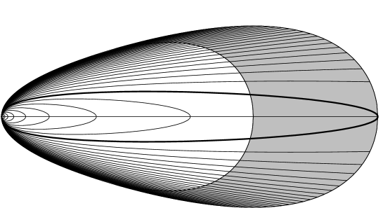
Figure 6: Equal observed synchrotron frequency contour lines, at a given observed time, for the BM solution. Each line represents a different value of $\phi$. The bold contour line is $\phi=1$. The lines are separated by a constant logarithmic interval in $\phi$: $\Delta Log_{10}(\phi)=0.05$ (the inner contour lines, which cross the LOS, represent $\phi<1$). The shaded region represents a finite shell of thickness $\Delta=R/4\gamma^{2}$ in the observer frame.

There are two opposing factors that determine the shape of the observed synchrotron frequency contour lines, that are depicted in Figure 6. The shift from the local frame to the observer frame, $\nu^{\prime}=\nu\gamma(1-\beta\nu)$, causes the frequency to decrease as one moves away from the LOS. However at earlier emission times, and at locations closer to the shock front, the typical synchrotron frequencies in the local frame are higher, and so is the Lorentz factor of the matter. This tends to increase the observed frequencies of photons that were emitted earlier (i.e. from the back of the “egg”) and closer to the shock (i.e. closer to the surface of the “egg”).

The result of these two opposing effects, for the BM solution, is that as one goes backwards along the LOS, to earlier emission times, the observed synchrotron frequency for a constant observed time is almost independent of $\chi$: $\nu_{syn}(LOS)\propto\chi^{-1/24}$. This explains the result for the flux arriving from the LOS (the dashed curve in Figure 5), namely that the peak flux is obtained at a frequency just slightly lower than $\nu_{T}$: $\phi_{peak}\cong 0.98$, and the light curve is only slightly rounded near the peak. The fact that $\nu_{min}<\nu_{T}$ along the LOS accounts for the fact that the peak flux is obtained at $\phi_{peak}<1$. The fact that the decrease in $\nu_{min}$ as one goes back along the LOS is very moderate, means that in order for the emitted radiation to be concentrated around a frequency substantially lower than $\nu_{T}$, one has to go very deep in the radial profile along the LOS to $r\ll R_{l}$. This implies that one gets far from the shock front (to $\chi\gg 1$), and therefore the contribution obtained to the total flux is small. For this reason $\phi_{peak}$ is very close to 1.

The observed flux from an infinitely thin shell peaks at $\phi_{peak}\cong 1.92$, and the light curve (or spectra) is quite rounded and flat near the peak (see the dotted line in Figure 5). This result can be understood by following the surface of the “egg” (see Figure 6). $\nu_{min}$ increases as one goes to the back of the “egg” (i.e. to earlier emission times) along it’s surface, and it does so much faster than it decreases when one goes back along the LOS. Therefore one gets a substantial contribution to the flux at $\phi>1$, before one gets too far back in the shell, where the total contribution to the flux drops considerably. This explains why the peak flux for an infinitely thin shell is obtained at a frequency significantly higher than $\nu_{T}$, whereas for the LOS it is obtained at a frequency only slightly lower than $\nu_{T}$.

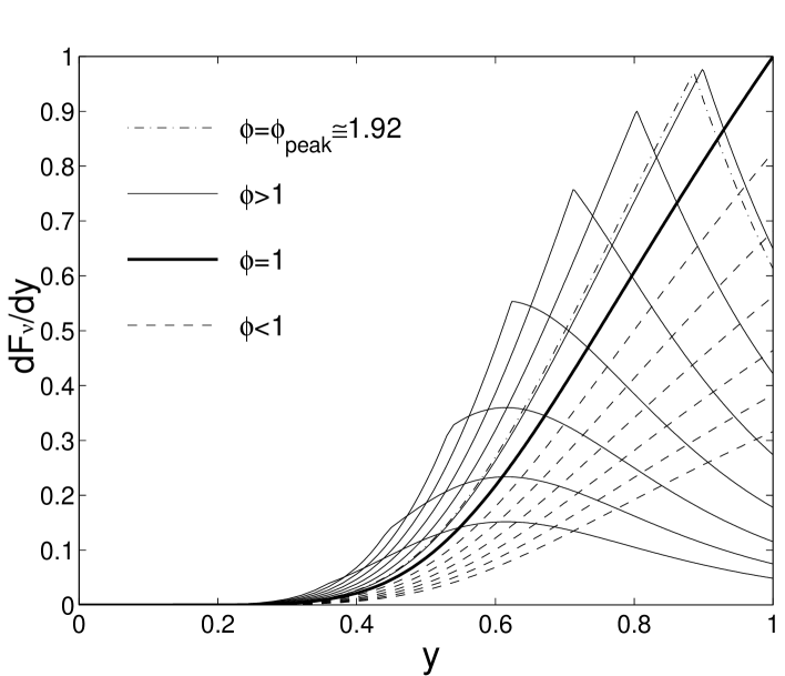
Figure 7: The contribution to the observed flux as a function of $y\equiv R/R_{l}$, for an infinitely thin shell. The different curves stand for $Log_{10}(\phi)=-1.5,-1.25,...,1.75$ and $\phi=\phi_{peak}\approx 1.92$. For $\phi<1$ the contribution peaks at the LOS ($y=1$), and for $\phi>1$ the contribution peaks at a lower value of $y$ as $\phi$ increases.

The contribution to the flux from an infinitely thin shell, as a function of the radius of the shell, for different values of $\phi$ is shown in Figure 7. The different curves can be looked upon as representing either different observed frequencies at the same observed time, or the same observed frequency at different observed times. One can see that for $\phi<1$ the contribution to the flux peaks at $y=1$ (the LOS), while for $\phi>1$ it peaks at smaller values of $y$. One can obtain the average radius contributing to a given $\phi$ in the following way:

$$\langle y\rangle={\int^{1}_{0}dy{dF(\phi)\over dy}y\over\int^{1}_{0}dy{dF(\phi)\over dy}}\ .$$ (25)

$\langle y\rangle(\phi)$ is shown in Figure 8. For $\phi<1$ one obtains that $\langle y\rangle$ is constant: $\langle y\rangle\cong 0.82$, while for $\phi>1$ there is a decrease in $\langle y\rangle$ until for $\phi\gg 1$ it reaches the limiting value: $\langle y\rangle\cong 0.65$. The same infinitely thin shell approximation was considered by Panaitescu & Mészáros (1998) and by Sari (1998). The values quoted by Panaitescu & Mészáros for $\langle y\rangle$ in the two limits of high and low frequencies are probably erroneous, and they are not consistent with the value they quote for the bolometric $\langle y\rangle$ (this inconsistency occurs only for the case we consider in this paper, of an adiabatic evolution of the shell, and neglecting electron cooling). The values obtained by Sari are slightly different than ours, since he considered emission from a shell consisting of a given element of matter.

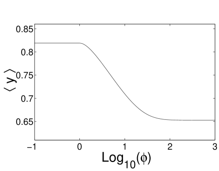
Figure 8: The average normalized radius $\langle y\rangle$ contributing to the observed flux at a given $\phi$, for an infinitely thin shell. $\langle y\rangle\approx 0.82$ for $\phi<1$, and it decreases as $\phi$ increases above $\phi=1$, until it reaches the limiting value of $\langle y\rangle\approx 0.65$ for large $\phi$, at around $\phi\sim 100$.

4 Alternative Magnetic Field models

Although the hydrodynamic profile is given by the BM solution, the structure and profile of the magnetic field are less clear. So far we have assumed that everywhere the magnetic field energy is a fixed fraction of the internal energy:

$$e^{\prime}_{B}\equiv{B^{2}\over 8\pi}=\epsilon_{B}e^{\prime}\ .$$ (26)

Since not much is known about the origin or spacial dependence of the magnetic field, we consider now two alternative models for the magnetic field. This can serve, in a way, as a test for the generality of our results, and it will expose any hidden fine tuning caused due to our previous magnetic field model, if one existed. We assume that each matter element acquires a magnetic field according to equation 26 when it passes the shock. The two alternative models are obtained by assuming that the magnetic field is either radial or tangential, and evolves according to the “frozen field” approximation.

Consider a small matter element, which passes the shock at a time $t_{0}$ in the observer frame. Just after it passes the shock it possesses a magnetic field $B_{0}$ (in the local frame) given by equation 26. We consider a cubic volume $V_{0}=L^{3}$ (in the local frame) with one face perpendicular to the radial direction. According to the BM solution, at a later time $t$ this matter element will be at $\chi=(R(t)/R(t_{0}))^{4}$, and it will occupy a box of a size $L_{rad}=\chi^{9/8}L$ in the radial direction, and a size $L_{\perp}=\chi^{1/4}L$ in the two tangential directions ($\hat{\phi}$ and $\hat{\theta}$). One also obtains that $B_{0}=B_{f}\chi^{3/8}$, where $B_{f}$ is the magnetic field at the front of the radial profile, just behind the shock, at the time $t$. We consider two possibilities for the direction of the magnetic field at $t_{0}$: a radial and a tangential magnetic field, $B_{rad}$ and $B_{\perp}$. Our previous “equipartition” model will be denoted simply by $B$. In both new cases the “frozen field” approximation implies that the magnetic field will remain in the same direction, while it’s magnitude changes in the following way:

$$B_{rad}=B_{f}\chi^{-1/8}\quad,\quad B=B_{f}\chi^{-17/24}\quad,\quad B_{\perp}=B_{f}\chi^{-1}\ .$$ (27)

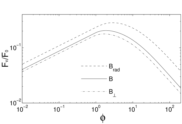
Figure 9: The observed flux for three different magnetic field models. $B_{rad}=B=B_{\perp}$ on the shock front, while behind the shock front $B_{rad}>B>B_{\perp}$.

TABLE 1
Features of the Light Curve and Spectra for
Different Models for the Magnetic Field. Magnetic Field Model $\phi_{peak}$ ${F_{\nu,max}\over F_{0}}$ $\phi_{-}$ $\phi_{+}$ $\phi_{+}\over\phi_{-}$ $T_{+}\over T_{-}$ $F_{extr}\over F_{0}$ $\phi_{extr}$ ${B_{\perp}}$ 1.67 0.178 0.157 15.9 101 21.7 0.273 4.12 ${B}$ 1.88 0.205 0.187 18 99 21.4 0.313 4.66 ${B_{rad}}$ 2.86 0.284 0.241 29 120 24.3 0.454 7.30

Table 1: $\phi_{peak}$, $F_{\nu,max}$, $F_{0}$, $\alpha$, $\phi_{-}$, $\phi_{+}$, $T_{-}$ and $T_{+}$ are all defined in the text. The last two columns refer to the point where the extrapolations of the power laws at high and low $\phi$ meet.

Using the general formula (equation 13), we obtain now the observed flux for $B_{rad}$ and $B_{\perp}$ (see Figure 9). Some of the features are summarized in Table 1. Since the emission from the shock front ($\chi=1$) is identical in all three cases, the results obtained for an infinitely thin shell in the previous section, including the dotted curve in Figure 5, are still valid here. This implies that the difference between the various curves in Figure 9 arises from the radial integration. Our previous model for the magnetic field led to an almost negligible effect of the radial profile (see Figure 5). Now we find that generally, the effect of the radial integration is comparable to that of the angular integration, as the flux for $B_{rad}$ and $B_{\perp}$ are substantially different than for an infinitely thin shell.

From equation 27, we can see that $B_{rad}$ implies a larger magnetic field than $B$, and therefore a larger total emission and higher emission frequencies, while $B_{\perp}$ implies a smaller magnetic field than $B$, and therefore a smaller total emission and lower emission frequencies. This is consistent with the results in Table 1, namely: $\phi_{peak,rad}>\phi_{peak}>\phi_{peak,\perp}$ and $F_{\nu,max,rad}>F_{\nu,max}>F_{\nu,max,\perp}$. An important feature that appears in all the magnetic field models we considered, is the flatness of the peak: $\phi_{+}/\phi_{-}\sim 100-120$ and $T_{+}/T_{-}\sim 21-24$ (see Table 1).

5 A Uniform Shell Approximation

In this section we consider a locally monochromatic emission. We consider a case where all the electrons at a certain point have the same Lorenz factor, which we chose to be the average Lorenz factor of the electrons at that point, given by equation 16. We take the angle $\alpha$ between the velocity of the electrons and the direction of the magnetic field in the local frame, to be the average value obtained for an isotropic velocity distribution: $\sin\alpha=\pi/4$. Under these assumptions, the emission from this point is at a single frequency, given by equation 17. The results are still expressed by the similarity variable $\phi\equiv\nu/\nu_{T}$, where in this section $\nu_{T}$ can be obtained from equation 20 by dropping the term involving $p$. The emitted power per unit volume per unit frequency in the local frame is given by:

$$P^{\prime}_{\nu^{\prime}}=n^{\prime}P^{\prime}_{e,av}\delta(\nu^{\prime}-\nu^{\prime}_{syn})\ ,$$ (28)

where $P^{\prime}_{e,av}$ is given by equation 16.

We now turn to calculate the observed flux due to this emission within a thin shell of matter, of finite thickness $\Delta$ in the observer frame. This case was calculated numerically by Waxman (1997c). He took: $\Delta=\zeta R/\gamma^{2}$, which corresponds in our notation to: $\chi_{max}(\zeta)=1+16\zeta$. We use equation 13, and integrate only up to $\chi_{max}(\zeta)$. Substituting $g(\chi)=1$ in equation 13, We obtained an analytic solution, and present it in Figure 10. We compare this both with a locally monochromatic emission from a BM profile (see Figure 12), and with synchrotron emission from a BM profile, obtained in section 3.

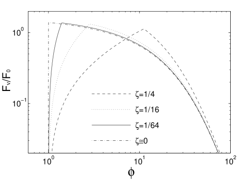
Figure 10: The observed flux from a uniform shell, for different values of the shell thickness in the observer frame: $\Delta\equiv\zeta R/\gamma^{2}$. The value of $\phi$ at the peak is a function of the shell thickness (see equation 29).

The flux obtained from a finite shell with a “cut” BM profile, is very similar to the flux from a full BM profile, shown in Figure 12, except that there is a cutoff at $\phi<(1-16\zeta)^{-1/24}$, due to the finiteness of the shell. The place of this cutoff is shown in Figure 12, for a few values of $\zeta$, including $\zeta\to 0$. Figure 10 depicts the observed flux from a uniform shell, for the same values of $\zeta$, and is considerably different. This large difference can be understood by looking at Figures 6 and 11, which depict the contour lines of equal observed emission frequency (which will be referred to as frequency contour lines) for the BM solution and for a uniform shell, respectively.

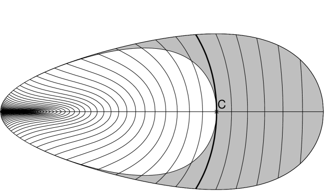
Figure 11: Equal observed synchrotron frequency contour lines, at a given observed time, for a uniform shell. The lines from right to left, represent: $\phi=5^{1/4},5^{2/4},5^{3/4},...$. The typical synchrotron frequency is larger than $\nu_{T}$ everywhere (everywhere $\phi>1$), and $\phi$ increases as one goes to the back (i.e. to the left) of the “egg” along the LOS, to smaller radii. The shaded region represents a finite shell of thickness $\Delta=R/4\gamma^{2}$ in the observer frame. The bold frequency contour line that touches the back of the shell on the LOS at point C, represents the frequency for which the flux from a uniform shell, considered in this section, peaks.

We now turn to Figure 12, which depicts the flux from a BM profile with a locally monochromatic emission. Normalizing according to the maximal flux, the flux from the LOS and the flux from an infinitely thin shell, practically coincide with the flux calculated from the general formula, for $\phi<1$ and $\phi>1$, respectively, and therefore are not shown separately. The flux peaks at $\phi_{peak}=1$ and drops sharply for $\phi<1$, while exhibiting a more moderate decrease for $\phi>1$. The frequency contour lines for the BM solution are nearly parallel to the LOS and their length within the thin shell (or up to a constant value of $\chi$) drops quickly to zero for $\phi<1$ (see Figure 6). This explains the quick drop (and eventual cutoff, for a finite shell) of the flux for $\phi<1$, and the fact that the peak flux is located at $\phi=1$. If one follows the shock front (i.e. the surface of the “egg”), one finds that the observed frequency increases as one moves from the LOS to the back of the “egg” (i.e. to smaller radii). This explains why we find a cut-off in the flux arriving from an infinitely thin shell, at frequencies smaller than $\nu_{T}$ ($\phi<1$). Since there is a sharp drop in the contribution to the flux as one goes back in the radial profile (away from the shock front), the flux at $\phi>1$ where there is a contribution from the front of the radial profile, is similar to the one obtained for an infinitely thin shell. For $\phi<1$,on the other hand, there is no contribution from the very front of the radial profile (near the shock front), and therefore the contribution from back the radial profile becomes apparent, and we obtain a result similar to the one obtained for the LOS.

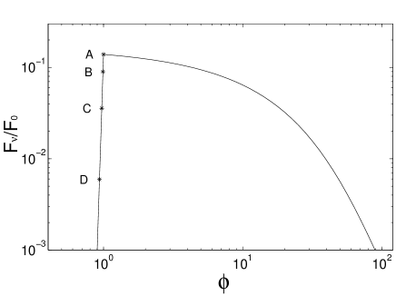
Figure 12: The observed flux from a locally monochromatic emission at the typical synchrotron frequency, using the BM solution. Since $\phi\propto\nu T^{3/2}$, this figure represents (with the correct scaling) both the light curve at a given frequency, and the spectrum at a given observed time. The peak flux is obtained at $\phi=1$, and the flux drops sharply for smaller $\phi$. If we consider only a slice of a BM profile, this introduces a cutoff at low $\phi$. This cutoff occurs at points A through D, for $\zeta\to 0$, $\zeta=1/64$, $\zeta=1/16$ and $\zeta=1/4$, respectively, where the shell thickness in the observer frame is $\Delta\equiv\zeta R/\gamma^{2}$.

The observed flux for a uniform shell is shown in figure 10. The shape of the light curve and the spectra, the shape and sharpness of the peak and the value of $\phi_{peak}$, all change considerably for different values of the shell thickness $\zeta$. The big difference compared to the results for a BM profile, can be understood by looking at Figure 11, which depicts the frequency contour lines for a uniform shell. The frequency contour lines are nearly perpendicular to the LOS and higher frequencies come from the back of the “egg” (i.e. from smaller radii). For this reason the flux vanishes for $\phi<1$ (see Figure 10). For every value of $\zeta$ there exists a critical frequency $\phi_{c}(\zeta)$ for which the frequency contour line touches the back of the shell, exactly on the LOS. This is demonstrated by the bold frequency contour line in Figure 11, which represents $\phi_{c}$ for $\zeta=1/4$, and touches the back of the shell exactly on the LOS at point C. For $\phi<\phi_{c}(\zeta)$ there is a sharp drop in the length of the frequency contour lines within the thin shell, that causes a sharp drop in the flux. For $\phi>\phi_{c}(\zeta)$ there is a moderate change in the length of the frequency contour lines within the thin shell, and the flux drops (though more moderately) for $\phi>\phi_{c}(\zeta)$ as well. This causes the peak flux to be exactly at $\phi_{c}(\zeta)$. From our analytical solution for a uniform thin shell we obtained a simple analytical expression for the time (or frequency) of the peak flux as a function of $\zeta$:

$$\phi_{peak}(\zeta)=\phi_{c}(\zeta)=(1+16\zeta)^{3/2}\ ,$$ (29)

The resulting spectra and light curve for a uniform shell are qualitatively different from those obtained when the hydrodynamical radial profile is considered. For a uniform shell, the rather arbitrary choice of $\zeta$ determines the time of the peak flux for a given observed frequency, and the peak is substantially sharper, with a smaller width at half maximum. The difference is even bigger if the results for a uniform shell are compared to those obtained for a realistic emission and a realistic hydrodynamic solution (the solid curve in Figure 5).

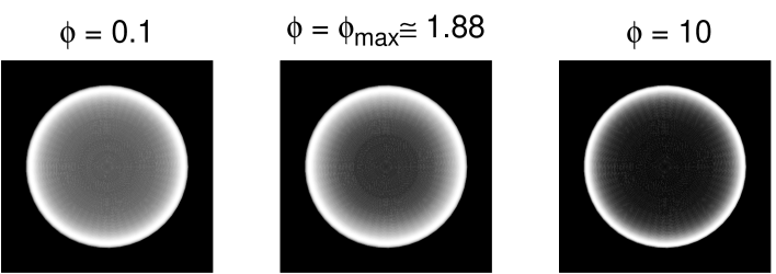
Figure 13: The observed image of a GRB afterglow, for different values of $\phi$. The different images can represent either the image at different frequencies at the same observed time, or the image at the same frequency at different observed times. In the latter case, one should also remember that the size of the observed image increases with the observed time as $R_{\perp,max}\propto T^{5/8}$. A larger value of $\phi$ represents a higher observed frequency or a later observed time. The image is brighter near the edge and dimmer near the center, and the contrast is higher at large values of $\phi$.

6 The Observed Image

We turn now to calculate the observed image, as seen by a distant observer. We consider the BM hydrodynamic solution. Substituting $g(\chi)=\chi^{-1}$ in equation 13 we obtain:

$$dF_{\nu}={8R_{l}^{3}\over D^{2}}{P^{\prime}y^{10}\chi\over(1+7\chi y^{4})^{2}}dyd\chi\ .$$ (30)

We calculate the surface brightness (energy per unit time per unit frequency per unit area perpendicular to the LOS) at a given arrival time $T$. The distance of a point from the LOS is given by:

$$R_{\perp}\equiv r\sin\theta\cong R_{l}y\sqrt{1-\mu^{2}}\cong{\sqrt{2}R_{l}\over 4\gamma_{l}}\sqrt{y-\chi y^{5}}\ .$$ (31)

The maximal value of $R_{\perp}$ is obtained on the surface of the “egg” (where $\chi=1$), implying $y=5^{-1/4}$. The observed image at a given observed time $T$ is restricted to a disk of radius $R_{\perp,max}\cong 4.14\gamma_{l}cT$ around the LOS. Using equation 12, we obtain an explicit expression for the BM solution:

$$R_{\perp,max}=3.91\times 10^{16}E_{52}^{1/8}n_{1}^{-1/8}T_{days}^{5/8}\rm{cm}\ .$$ (32)

We calculate the surface brightness within this disk, and find it useful to work with the variable: $x\equiv R_{\perp}/R_{\perp,max}$. The differential of the area on this disk is given by:

$$dS_{\perp}=2\pi R_{\perp}dR_{\perp}\equiv 2\pi R^{2}_{\perp,max}xdx\ .$$ (33)

Using equation 31, we obtain from equation 30:

$${dF_{\nu}\over dS_{\perp}}={4\over\pi}\left({R_{l}\over D}\right)^{2}{1\over cT}{P^{\prime}y^{5}\chi\over(1+7\chi y^{4})^{2}}dy\ ,$$ (34)

from which we obtain after integration, the surface brightness as a function of $R_{\perp}$. In this expression, $\chi$ should be taken as a function of $y$ for a given $x$, according to equation 31. The limits of the integration over $y$ are determined from the condition $\chi>1$.

TABLE 2
Features of the Observed Image.
Magnetic Field ${\rm SB}(x=0)/{\rm SB}_{max}$ $\phi<1$ $\phi\gg 1$ Model $\phi<1$ $\phi\gg 1$ $x_{peak}$ $\Delta x$ $x_{peak}$ $\Delta x$ ${B_{\perp}}$ 0.32 0.034 0.95 0.263 0.96 0.151 ${B}$ 0.34 0.039 0.94 0.296 0.95 0.178 ${B_{rad}}$ 0.39 0.065 0.93 0.403 0.90 0.290

Table 2: . We define $\Delta x\equiv x_{+}-x_{-}$, where $x_{+}>x_{-}$ are the values of $x\equiv R_{\perp}/R_{\perp,max}$ at which the surface brightness (SB) drops to half of it’s maximal value. $\Delta x$ is an estimate for the width of the bright ring that appears on the outer edge of the image. $x_{peak}$ is the value of $x$ for which the maximal SB is obtained, and it’s values indicate that the SB peaks near the outer edge of the image. It is evident that the contrast between the center and the edge of the image is considerably larger for high frequencies (or late times) than for low frequencies (or early times).

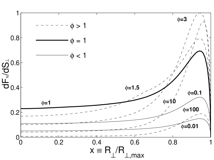
Figure 14: The observed surface brightness as a function of $x\equiv R_{\perp}/R_{\perp,max}$, for different values of $\phi$. The surface brightness peaks near the outer edge of the image, drops sharply towards the edge ($x=1$) and decreases more gradually towards the center. The normalization preserves the correct ratio between the absolute surface brightness, for the different values of $\phi$, which decreases both for low and for high values of $\phi$.

We calculated the surface brightness for several values of $\phi$, and as before, the different images can be viewed as either the observed images at a given observed time at different observed frequencies, or as the observed images at a given frequency at different observed times. The observed images are quite similar for the different magnetic field models we considered, and therefore we present detailed results only for $B$ (figures 13 and 14), and summarize the features of the images obtained for $B_{rad}$, $B$ and $B_{\perp}$ in Table 2.

The observed image is bright near the edge and dimmer at the center. At high values of $\phi$ (high frequencies or late observed times) the surface brightness at the center is only a few percent of the maximal surface brightness, which is obtained near the edge ($x\sim 0.93-0.95$), and a bright ring is clearly seen with a sharp edge on the outer side and a more gradual decrease in the surface brightness towards the center. At $\phi<1$ (low frequencies or early observed times) the surface brightness at the center is around $0.32-0.39$ of the maximal surface brightness, and though the image is brighter near the edge, the center should be visible as well (see the left image in Figure 13).

The transition in the distribution of the relative surface brightness along the observed image, between the limiting cases of small and large $\phi$, occurs over one order of magnitude in $\phi$: $1<\phi<10$. The relative surface brightness hardly changes beyond this region (though the absolute surface brightness drops both for low and for high values of $\phi$, due to the drop in the observed flux).

The fact that at a given observed time, the relative surface brightness at the center of the image is smaller for high frequencies than it is for low frequencies, may be intuitively understood: for high frequencies the emittance decays in time, and is therefore lower at large radii, which correspond to small values of $x\propto R_{\perp}$, which are located at the center of the image.

7 Discussion

We have derived a formula for the observed flux from a relativistically moving system. Using this formula, we considered the emission from the whole volume behind a spherical relativistic blast wave, expanding into a cold uniform medium. We have considered an adiabatic evolution and used the self similar hydrodynamical solution of Blandford & McKee (1976) to describe the matter behind the shock.

We have considered synchrotron emission from a power law distribution of electrons, using a realistic local emissivity, which depends on the local hydrodynamic parameters. We have obtained expressions for the frequency at which the observed flux peaks at a given observed time, and for the value of the peak flux (equations 23 and 24). The value we obtained for the peak frequency at a given observed time is a factor of $\sim 1.8$ smaller than the value obtained by Sari, Piran & Narayan (1998), a factor of $\sim 2.5$ (for $p=2.5$) smaller than the value obtained by Wijers & Galama (1998), and a factor of $\sim 35$ (for $p=2.5$) smaller than the value obtained by Waxman (1997b). The large difference from the result obtained by Waxman is partly due to the fact that he took the peak frequency to be at the synchrotron frequency of an average electron $\nu_{syn}(\langle\gamma_{e}\rangle)$, while the peak frequency is actually obtained much closer to $\nu_{syn}(\gamma_{min})$, i.e. the synchrotron frequency of an electron with the minimal Lorentz factor. The value we obtained for the peak flux is a factor of $\sim 1.9$ (for $p=2.5$) smaller than the value obtained by Wijers & Galama (1998), a factor of $\sim 5.1$ larger than the value obtained by Waxman (1997b), and a factor of $\sim 6.5$ smaller than the value obtained by Sari, Piran & Narayan (1998).

We have shown that both the light curve and the spectra are flat near the peak. The flux at a given observed time drops to half it’s maximal value at around one order of magnitude from the peak frequency, on either side. The flux at a given observed frequency drops to half it’s maximal value at about a factor of $\sim 5$ before and after the time of the peak flux. This result was obtained for all the magnetic field models we considered, and it therefore seems to be of quite a general nature. Our calculations were made using an approximation for the local emissivity that is obtained from an exact synchrotron emission. We expect that without this approximation the values of the peak flux and the peak frequency should be somewhat lower, and the light curve and the spectra should be even more rounded and flat near the peak. We estimated that these effects should be small.

In contrast to the flatness of the peak, discussed above, GRB970508 displayed a sharp rise in the optical flux, immediately followed by a power law decay (Sokolov et. al. 1997). Sari, Piran & Narayan (1998) considered both radiative and adiabatic evolution of the blast wave, and found that the steepest rise in the flux occurs before the peak, for an adiabatic evolution and slow cooling of the electrons, which is the case discussed in this paper. This steepest rise is $T^{1/2}$, and as we have shown in this paper, the rise in the flux decreases as the peak is approached, and the peak itself is quite flat. We obtained $T_{+}/T_{-}\sim 21-24$, which indicates a flat peak, while GRB970508 displayed $T_{+}/T_{-}<3$. This rules out the interpretation of the optical peak of GRB970508 as the peak of the light curve, predicted by the existing fireball models. It therefore appears that another explanation is needed.

We have considered a locally monochromatic emission, at the typical synchrotron frequency, obtained from the relevant hydrodynamic parameters. We have shown that when this emission is applied to the BM solution, the observed flux peaks at the observed emission frequency of the matter just behind the shock, on the LOS ($\phi_{peak}=1$). There is a sharp drop in the flux below this frequency, and a gradual decrease above it. When this emission is applied to a uniform shell (Waxman 1997b) the results change drastically. In particular the location of the peak flux depends critically on the width of the shell $\zeta$ (see equation 29), which is chosen quite arbitrarily.

The image of a GRB afterglow looks like a ring, even when emission is considered from the whole volume behind the shock front. Similar results were obtained for more simplified models (Waxman 1997b, Sari 1998, Panaitescu & Mészáros 1998). The image is bright near the edge and dimmer at the center. The contrast in the surface brightness between the center and the edge of the image is larger for high frequencies (optical and x-ray) and the ring is narrower, while for low frequencies (as long as self absorption is not significant) the contrast is smaller and the ring is wider. Radio wave-bands can be considered as “low frequencies” for the first few months. The best available resolution is obtained in radio frequencies, and the afterglow of a future nearby GRB ($z\sim 0.2$) might be resolved. This theory predicts that in early times, when $\nu_{radio}<\nu_{peak}$ the image should appear as a relatively wide ring with a relatively small contrast, while for later times where $\nu_{radio}>\nu_{peak}$ (as long as the relativistic regime is not exceeded) the image should appear as a narrow ring and posses a large contrast.

The observed image has been calculated, considering emission only from the surface of the shock front (Sari 1998). This yielded a surface brightness diverging at $R_{\perp,max}$. This divergence is an artifact of the assumption that the radiation is emitted from a two dimensional surface. Other features of the image, such as the difference between high and low frequencies, are quite similar in the more simplified analysis.

This research was supported by NASA Grant NAG5-3516, and a US-Israel Grant 95-328. Re’em Sari thanks The Clore Foundation for support.

References

- [1] Blandford, R. D. & McKee, C. F. 1976, Phys. of fluids,19, 1130.
- [2] Katz, J. & Piran, T. 1997, ApJ, 490, 772.
- [3] Mészáros, P. & Rees, M. 1997, ApJ, 476, 232.
- [4] Panaitescu, A. & Mészáros, P. 1998, ApJ, 493, L31.
- [5] Piran, T. 1994, in AIP Conference Proceedings 307, Gamma-Ray Bursts, Second Workshop, Huntsville, Alabama, 1993, eds. G. J. Fishman, J. J. Brainerd, & K. Hurley (New York: AIP), p. 495.
- [6] Rybici, G.B. & lightman, A.P. 1979, Radiative Processes in Astrophysics, Wiley-Interscience, Chap. VI
- [7] Rees, M. 1966, Nature, 211, 468.
- [8] Sari, R. 1997, ApJ, 489, L37.
- [9] Sari, R. 1998, ApJ, 494, L49
- [10] Sari, R., Piran, T. & Narayan, R. 1998, ApJ, 497, L17.
- [11] Sokolov et. al. 1997, astro-ph/9706141.
- [12] Waxman, E. 1997a, ApJ, 485, L5.
- [13] Waxman, E. 1997b, ApJ, 489, L33.
- [14] Waxman, E. 1997c, ApJ, 491, L19.
- [15] Wijers, R.A.M.J. & Galama, T.J. 1998, astro-ph/9805341.