The Thermal Evolution of the Postshock Layer
in Pregalactic Clouds

Abstract

We re-examine the thermal evolution of the postshock layer in primordial gas clouds. Comparing the time scales, we find that the evolutionary paths of postshock regions in primordial gas clouds can be basically understood in terms of the diagram drawn in the ionization degree vs temperature plane. The results obtained from the diagram are independent of the density in the case that we do not include photodissociation and photoionization. We also argue that the diagram is not only relevant to the case of the steady postshock flow, but also to the isochorically cooling gas.

1 Introduction

The thermal evolution of primordial gas clouds has been investigated by many authors. [15, 24, 3, 17, 9, 20, 29] Almost all of those studies have been concerned with the formation of various kinds of galaxies, or primordial stars. In those papers, galaxies are assumed to grow out of small density perturbations present in the early universe. Because of the coldness of the growing density perturbations, the formed clouds, which are the progenitors of galaxies, experience strong shock heating at the bouncing epoch. Shock heating is also expected in the hierarchical clustering scenario of structure formation. In this case, shocks are expected in the collision between two clouds which are trapped in the gravitational potential well associated with the larger structure.

In any case, shock heating is expected in the era of galaxy formation. The spatial structure and the thermal evolution of the postshock layer in primordial gas clouds were investigated by many authors. [8, 26, 27, 14, 23, 10, 1, 30] In those studies the common and the most important point is the over production of hydrogen molecules. For example, in Shapiro and Kang [23] (hereafter SK), the thermal evolution of steady postshock flow is investigated. They found that the postshock flow cools down so fast that the recombination process cannot catch up with the cooling. As a result, the ionization degree remains high ($y_{e}\sim 10^{-3}$), even when the temperature has dropped below $10^{4}\;{\rm K}$. Feeded these “relic” electrons, hydrogen molecules form through the processes

$${\rm H+e\rightarrow H^{-}+\gamma},$$ (1)

$${\rm H+H^{-}\rightarrow H_{2}+e}.$$ (2)

SK stressed the importance of these non-equilibrium cooling processes and the difficulties of describing these processes with a finite-difference scheme.

SK calculated the cases corresponding to the shock velocity in the range ($50{\rm km/s}-300{\rm km/s}$). In all cases, the resulting fractions of hydrogen molecules are $\sim 10^{-3}$, irrespective of the initial shock velocities. Ionization degrees are also independent of the initial shock velocities for the same temperature if $T\ll 10^{4}$ K. Surprisingly, the convergence is quite good, though chemical equilibrium is not achieved throughout almost the entire evolutionary path. Therefore there may be a clear explanation for the independence of the initial shock velocity.

In this paper we re-examine the thermal evolution of the postshock layer in primordial gas clouds. To elucidate the convergence of the hydrogen molecule fraction in the course of the evolution of the postshock region, we simply compare several important time scales (§2). We find that we can predict the thermal evolution of the postshock layer for any initial conditions in a diagram of the ionization degree versus temperature. In §3 we also test the results obtained in §2 by comparing the results with those of numerical calculations for the steady postshock flow. In §4 we show that the thermal evolution of isochorically cooling gas is very similar to that of steady postshock flow. The remainder of the section is devoted to the further discussion and summary.

2 TIME SCALES

In this section we compare the time scales which are essential to the thermal evolution of the postshock layer in primordial gas clouds. First of all, we enumerate the definition of the time scales

$$t_{\rm cool} \equiv C_{p,v}\frac{\rho kT}{\mu m_{p}\Lambda},$$ (3)

$$t_{\rm ion} \equiv \frac{n_{p}}{k^{\rm ion}n_{\rm H}n_{e}}=\frac{1}{k^{\rm ion}n_{N}(1-y_{e})},$$ (4)

$$t_{\rm rec} \equiv \frac{n_{p}}{k^{\rm rec}n_{e}n_{p}}=\frac{1}{k^{\rm rec}n_{N}y_{e}},$$ (5)

$$t_{\rm dis} \equiv \frac{n_{\rm H_{2}}}{\sum_{i}k^{\rm dis}_{i}\;n_{\rm H_{2}}n_{i}}=\frac{1}{\sum_{i}k^{\rm dis}_{i}\;n_{N}y_{i}},$$ (6)

$$t_{\rm for} \equiv \frac{n_{\rm H_{2}}}{\sum_{ij}k^{\rm for}_{ij}\;n_{i}n_{j}}=\frac{y_{\rm H_{2}}}{\sum_{ij}k^{\rm for}_{ij}\;n_{N}y_{i}y_{j}}.$$ (7)

Here $t_{\rm cool},t_{\rm ion},t_{\rm rec},t_{\rm dis}$ and $t_{\rm for}$ denote the time scales of cooling, ionization, recombination, ${\rm H_{2}}$ dissociation, and ${\rm H_{2}}$ formation, respectively. $n_{N}$, $n_{i}$, $y_{i}~{}(\equiv n_{i}/n_{N})$, $k^{X}$, $\rho$, $\mu$ and $m_{p}$ are the number density of nucleons, the number density of the $i$th species, the fraction of ith species, the chemical reaction rate coefficient of the “$X$” process, the mass density, the mean molecular weight, and proton mass, respectively. $\Lambda$ denotes the net cooling rate which includes radiative and chemical cooling/heating, assuming that the system is optically thin for cooling photons. This assumption is valid for subgalactic clouds with mass $10^{6}-10^{8}M_{\odot}$ and whose densities are smaller than $\sim 10^{8}\;{\rm cm^{-3}}$. If a cloud violates this condition, the system could be optically thick for the H₂ cooling line photons. Another assumption is that the primordial gas does not contain helium but only hydrogen. This assumption affects the mean molecular weight and the cooling rate at high temperature $(T\sim 10^{5}\;{\rm K})$. However, these are minor effects for the thermal evolution of primordial gas clouds at lower temperature ($T\mathrel{\mathchoice{\lower 2.15277pt\vbox{\halign{$\mathsurround 0pt \displaystyle\hfil#\hfil$\cr<\crcr\sim\crcr}}}{\lower 2.15277pt\vbox{\halign{$\mathsurround 0pt \textstyle\hfil#\hfil$\cr<\crcr\sim\crcr}}}{\lower 2.15277pt\vbox{\halign{$\mathsurround 0pt \scriptstyle\hfil#\hfil$\cr<\crcr\sim\crcr}}}{\lower 2.15277pt\vbox{\halign{$\mathsurround 0pt \scriptscriptstyle\hfil#\hfil$\cr<\crcr\sim\crcr}}}}10^{4}$ K), which we are especially interested in. Therefore, for simplicity we do not include helium. $C_{p,v}$ denotes the heat capacity of the gas cloud. If the gas evolves isobarically, $C_{p}$ is chosen, and if the cloud is isochoric, $C_{v}$ is chosen. These quantities are expressed in terms of $\gamma$ as

$$C_{p} \equiv \frac{\gamma}{\gamma-1},$$ (8)

$$C_{v} \equiv \frac{1}{\gamma-1},$$ (9)

where $\gamma=5/3$ for an ideal gas without molecules. When we are interested in a steady flow, the postshock layer is almost isobaric (see Appendix B).

The ionization time scale (Eq. (4)) is defined as the variation time scale of $y_{e}$. Another possibility is definition in terms of $1-y_{e}$. However, it is not appropriate for the problem we are now interested in, because the magnitude of ionization degree itself is important for the formation of hydrogen molecules. In any case, comparing these five time scales we can find the fastest process without solving detailed time dependent differential equations.

We should remark that all of these time scales are proportional to $\rho^{-1}$ if the cooling rate and other reaction rates are proportional to $\rho^{2}$. The dominant component of the cooling changes according to the temperature. Below $10^{4}\;{\rm K}$, the ${\rm H_{2}}$ line emission dominates the total cooling of the cloud. In this process, the cooling rate is proportional to the number density of the hydrogen molecules at the excited levels whose fraction is proportional to $\rho$. [7] Hence, the cooling time scale is proportional to $\rho^{-1}$ for $T\mathrel{\mathchoice{\lower 2.15277pt\vbox{\halign{$\mathsurround 0pt \displaystyle\hfil#\hfil$\cr<\crcr\sim\crcr}}}{\lower 2.15277pt\vbox{\halign{$\mathsurround 0pt \textstyle\hfil#\hfil$\cr<\crcr\sim\crcr}}}{\lower 2.15277pt\vbox{\halign{$\mathsurround 0pt \scriptstyle\hfil#\hfil$\cr<\crcr\sim\crcr}}}{\lower 2.15277pt\vbox{\halign{$\mathsurround 0pt \scriptscriptstyle\hfil#\hfil$\cr<\crcr\sim\crcr}}}}10^{4}\;{\rm K}$ as in Eq. (3). The cooling process in $10^{4}\;{\rm K}\mathrel{\mathchoice{\lower 2.15277pt\vbox{\halign{$\mathsurround 0pt \displaystyle\hfil#\hfil$\cr<\crcr\sim\crcr}}}{\lower 2.15277pt\vbox{\halign{$\mathsurround 0pt \textstyle\hfil#\hfil$\cr<\crcr\sim\crcr}}}{\lower 2.15277pt\vbox{\halign{$\mathsurround 0pt \scriptstyle\hfil#\hfil$\cr<\crcr\sim\crcr}}}{\lower 2.15277pt\vbox{\halign{$\mathsurround 0pt \scriptscriptstyle\hfil#\hfil$\cr<\crcr\sim\crcr}}}}T\mathrel{\mathchoice{\lower 2.15277pt\vbox{\halign{$\mathsurround 0pt \displaystyle\hfil#\hfil$\cr<\crcr\sim\crcr}}}{\lower 2.15277pt\vbox{\halign{$\mathsurround 0pt \textstyle\hfil#\hfil$\cr<\crcr\sim\crcr}}}{\lower 2.15277pt\vbox{\halign{$\mathsurround 0pt \scriptstyle\hfil#\hfil$\cr<\crcr\sim\crcr}}}{\lower 2.15277pt\vbox{\halign{$\mathsurround 0pt \scriptscriptstyle\hfil#\hfil$\cr<\crcr\sim\crcr}}}}10^{5}\;{\rm K}$ is dominated by the bound-bound transition of the hydrogen atoms, and the number of the excited hydrogen atoms is determined by the collisions with other atoms. Therefore, the cooling rate is proportional to the square of the total density. For higher temperature ($T\mathrel{\mathchoice{\lower 2.15277pt\vbox{\halign{$\mathsurround 0pt \displaystyle\hfil#\hfil$\cr>\crcr\sim\crcr}}}{\lower 2.15277pt\vbox{\halign{$\mathsurround 0pt \textstyle\hfil#\hfil$\cr>\crcr\sim\crcr}}}{\lower 2.15277pt\vbox{\halign{$\mathsurround 0pt \scriptstyle\hfil#\hfil$\cr>\crcr\sim\crcr}}}{\lower 2.15277pt\vbox{\halign{$\mathsurround 0pt \scriptscriptstyle\hfil#\hfil$\cr>\crcr\sim\crcr}}}}10^{5}\;{\rm K}$), the free-free emission by the collision between ions and electrons dominates the energy radiated away from the cloud. In any case, the cooling rate is proportional to $\rho^{2}$, and the cooling time is proportional to $\rho^{-1}$. The chemical reaction rates are proportional to $\rho^{2}$ if the reactions are dominated by the collisional processes. Photoionization and H₂ photodissociation processes by UV photons emitted from the postshock hot region could affect the ionization rates and the H₂ dissociation rates in the postshock regions. If these radiative reactions dominate the other reactions, total reaction rates will not be proportional to $\rho^{2}$, because photoionization and H₂ photodissociation processes are not collisional. Kang and Shapiro[10] investigated this problem. The figures in their paper indicate that the effects caused by the internally produced photons are not too large to dominate that of the collisional processes. Hence, as a 0th-order approximation, we neglect the photoionization and the H₂ photodissociation processes in this paper.

As a result, the ratio of any two time scales is independent of the total density, and they are determined by the temperature and the chemical compositions ($y_{e}$ and $y_{\rm H_{2}}$). As will be discussed later, $y_{\rm H_{2}}$ is almost always determined by $y_{e}$ and $T$. Therefore, the ratio of any two time scales just depends on $T$ and $y_{e}$. In the following sections, we compare the time scales individually.

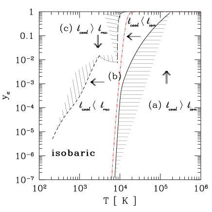
Figure 1: The $y_{e}$-$T$ plane is divided into several regions in which the ratio of the time scales are differ. The arrows in the plane denote the directions of the evolution of the postshock layer. The dot–short-dashed curve where the equality $t_{\rm rec}=t_{\rm ion}$ holds. Region (a) in which the condition $t_{\rm ion}<t_{\rm cool}$ holds is bounded by the solid line. In this region, the system evolves upward in the $y_{e}$-$T$ diagram. In region (b), the conditions $t_{\rm cool}<t_{\rm ion},~{}t_{\rm rec}$ always holds. Therefore the temperature drops down before the system is further ionized or recombines. In region (c) we have $t_{\rm rec}<t_{\rm cool}$, and the system evolves downward. Region (c) is bounded by the dotted line, short-dashed line and the long-dashed line. Those three lines denote the boundary on which the condition $t_{\rm cool}=t_{\rm rec}$ holds. The long-dashed line was calculated by assuming that the cooling rate is dominated by the hydrogen line cooling. The dotted line was calculated assuming chemical equilibrium of the hydrogen molecules, and the short-dashed line was calculated with $y_{\rm H_{2}}=10^{-3}$, which corresponds to the frozen value of the hydrogen molecules for a shock velocity higher than $\sim 30\;{\rm km/s}$, see also Fig. 2.

2.1 Ionization and cooling

First, we investigate the case $t_{\rm ion}<t_{\rm rec}$, which corresponds to higher temperature ($T\mathrel{\mathchoice{\lower 2.15277pt\vbox{\halign{$\mathsurround 0pt \displaystyle\hfil#\hfil$\cr>\crcr\sim\crcr}}}{\lower 2.15277pt\vbox{\halign{$\mathsurround 0pt \textstyle\hfil#\hfil$\cr>\crcr\sim\crcr}}}{\lower 2.15277pt\vbox{\halign{$\mathsurround 0pt \scriptstyle\hfil#\hfil$\cr>\crcr\sim\crcr}}}{\lower 2.15277pt\vbox{\halign{$\mathsurround 0pt \scriptscriptstyle\hfil#\hfil$\cr>\crcr\sim\crcr}}}}10^{4}$ K), and we compare the time scale of ionization with that of cooling. As mentioned previously, the ratio $t_{\rm ion}/t_{\rm cool}$ does not depend on $\rho$, but on the ionization degree $y_{e}$ and temperature $T$, because both ionization and cooling, which are dominated by atomic hydrogen line cooling, occur through two-body collisions. Hence the ratio $t_{\rm ion}/t_{\rm cool}$ is determined at each point on the $y_{e}$-$T$ plane independently of the density. The line along which $t_{\rm ion}/t_{\rm cool}$ is equal to unity is indicated by the solid line in Fig. 1. If the initial conditions are given below the line, the system is ionized before it cools down, because $t_{\rm ion}/t_{\rm cool}<1$. Otherwise, the system cools before it is ionized. The expected evolutionary path is also expressed by the arrows in Fig. 1.

2.2 Recombination and cooling

Next we investigate the case $t_{\rm rec}<t_{\rm ion}$, which corresponds to lower temperature, and examine the balance between the recombination process and the cooling process. The recombination process is important for $T\mathrel{\mathchoice{\lower 2.15277pt\vbox{\halign{$\mathsurround 0pt \displaystyle\hfil#\hfil$\cr<\crcr\sim\crcr}}}{\lower 2.15277pt\vbox{\halign{$\mathsurround 0pt \textstyle\hfil#\hfil$\cr<\crcr\sim\crcr}}}{\lower 2.15277pt\vbox{\halign{$\mathsurround 0pt \scriptstyle\hfil#\hfil$\cr<\crcr\sim\crcr}}}{\lower 2.15277pt\vbox{\halign{$\mathsurround 0pt \scriptscriptstyle\hfil#\hfil$\cr<\crcr\sim\crcr}}}}10^{4}\;{\rm K}$ . When $T\mathrel{\mathchoice{\lower 2.15277pt\vbox{\halign{$\mathsurround 0pt \displaystyle\hfil#\hfil$\cr<\crcr\sim\crcr}}}{\lower 2.15277pt\vbox{\halign{$\mathsurround 0pt \textstyle\hfil#\hfil$\cr<\crcr\sim\crcr}}}{\lower 2.15277pt\vbox{\halign{$\mathsurround 0pt \scriptstyle\hfil#\hfil$\cr<\crcr\sim\crcr}}}{\lower 2.15277pt\vbox{\halign{$\mathsurround 0pt \scriptscriptstyle\hfil#\hfil$\cr<\crcr\sim\crcr}}}}10^{4}\;{\rm K}$, the line cooling of the hydrogen molecules dominates the atomic hydrogen line cooling. Therefore the ratio $t_{\rm rec}/t_{\rm cool}$ depends not only on the ionization degree and the temperature but also on the fraction of hydrogen molecules. In order to draw the line $t_{\rm rec}/t_{\rm cool}=1$ in the $y_{e}$-$T$ plane, we need information on the fraction of hydrogen molecules. As will be discussed in the next subsection, the fraction of ${\rm H_{2}}$ is determined by the chemical equilibrium above $\sim 10^{4}\;{\rm K}$. Then, it is approximately frozen below $\sim 4\times 10^{3}\;{\rm K}$ through the evolutionary course with cooling. The line along which $t_{\rm rec}/t_{\rm cool}=1$ is satisfied is drawn in Fig. 1. In the region above the line, the system recombines before it cools down, and below the line, the system cools down before the recombination proceeds. The expected evolutionary path is also indicated in Fig. 1 by the arrows.

2.3 Fraction of ${H_{2}}$

Here we investigate whether or not ${\rm H_{2}}$ is in chemical equilibrium. If ${\rm H_{2}}$ is in chemical equilibrium (with given $T$ and $y_{e}$), the cooling time is always determined by just $T$ and $y_{e}$. As a result, the thermal evolution of the system is completely determined in the $y_{e}$-$T$ plane. The fraction of hydrogen molecules is roughly determined by estimating $t_{\rm dis}$ and $t_{\rm for}$, which denote the time scale of the dissociation and the formation of hydrogen molecules. If at least one of the two time scales is shorter than the other time scales, $t_{\rm cool}$ and $t_{\rm rec}$, the fraction of hydrogen molecules changes toward the chemical equilibrium value. Hence, the ratios $t_{\rm dis}/t_{\rm cool,rec}$ and $t_{\rm for}/t_{\rm cool,rec}$ should be examined.

First of all, we comment on the important properties of $t_{\rm dis}$ and $t_{\rm for}$. The time scale of dissociation is independent of $y_{\rm H_{2}}$, the fraction of hydrogen molecules. On the other hand, $t_{\rm for}$ is proportional to $y_{\rm H_{2}}$. Then both the time scales given in terms of their equilibrium values are

$$t_{\rm dis} = t_{\rm dis}^{eq},$$ (10)

$$t_{\rm for} = t_{\rm for}^{eq}\frac{y_{\rm H_{2}}}{y_{\rm H_{2}}^{\it eq}},$$ (11)

where the superscript eq denotes the value at which the hydrogen molecules are in chemical equilibrium for a given electron abundance and temperature. Here, the electron abundance is not an equilibrium value in general. Therefore the relation $t_{\rm for}^{eq}=t_{\rm dis}^{eq}$ holds.

Suppose that we know the important time scale ($t_{\rm sys}$) which characterize the evolution of the system. It could be $t_{\rm rec},t_{\rm cool}$, and so on. If $t_{\rm sys}$ is independent of $y_{\rm H_{2}}$, we have general arguments as follows: 1) In the case $y_{\rm H_{2}}>y_{\rm H_{2}^{\it eq}}$, dissociation proceeds faster than the formation process. Hence, $t_{\rm dis}$ controls the change of $y_{\rm H_{2}}$. This is the reason we do not have to be concerned about $t_{\rm for}$. Since $t_{\rm dis}$ is independent of $y_{\rm H_{2}}$, $y_{\rm H_{2}}$ converges to $y_{\rm H_{2}}^{\it eq}$ if $t_{\rm dis}<t_{\rm sys}$ is satisfied. 2) If $y_{\rm H_{2}}<y_{\rm H_{2}}^{\it eq}$, $y_{\rm H_{2}}$ is controlled by the time scale $t_{\rm for}$, because the system will try to recover the fraction of ${\rm H_{2}}$ which is smaller than the equilibrium value. The maximal value of $t_{\rm for}$ is the equilibrium value, since $t_{\rm for}$ is proportional to $y_{\rm H_{2}}$(Eq.(11)). Therefore, if $t_{\rm sys}>t_{\rm for}^{eq}(=t_{\rm dis})$, $t_{\rm sys}$ is always greater than $t_{\rm for}$. As a result, $t_{\rm sys}>t_{\rm dis}$ is a sufficient condition for the system to maintain the chemical equilibrium of hydrogen molecules. In the following, we look into the concrete cases that the interesting time scales are $t_{\rm rec}$ and $t_{\rm cool}$.

Figure 2: (a) The $y_{e}$-$T$ plane is divided into two regions, where chemical equilibrium is achieved for the fraction of hydrogen molecules and where not. The solid boundary of the shaded region is determined by the condition $t_{\rm cool}=t_{\rm dis}$. The long-dashed line denotes the boundary at which $t_{\rm rec}=t_{\rm dis}$ is satisfied. In the shaded region, the chemical equilibrium of hydrogen molecules breaks down, and the fraction $y_{\rm H_{2}}\equiv n_{\rm H_{2}}/n_{\rm H}$ freezes as the temperature and/or ionization degree drops. The dotted lines labeled as $100\;{\rm km/s}$ and $20\;{\rm km/s}$ denote the evolutionary path of $y_{e}$. (b) The equilibrium and non-equilibrium fraction of hydrogen molecules are drawn in $y_{\rm H_{2}}$-$T$ plane. The solid lines labeled $100\;{\rm km/s}(y_{\rm H_{2}})$ and $20\;{\rm km/s}(y_{\rm H_{2}})$ denote the dynamically calculated evolutionary path of the fraction of hydrogen molecules. The short-dashed lines which are labeled as $100\;{\rm km/s}(y_{\rm H_{2}}^{eq})$ and $20\;{\rm km/s}(y_{\rm H_{2}}^{eq})$ denote the fraction of ${\rm H_{2}}$ calculated assuming the chemical equilibrium of hydrogen molecules with dynamically calculated electron density.

2.3.1 $t_{\rm dis,for}$ vs $t_{\rm rec}$

First, let us investigate the chemical equilibrium of hydrogen molecules compared to the recombination process. In other words, we investigate the magnitudes of $t_{\rm dis}/t_{\rm rec}$ and $t_{\rm for}/t_{\rm rec}$. As discussed above, when we compare $t_{\rm dis}$ and $t_{for}$ with other time scales which do not depend on $y_{\rm H_{2}}$, we do not have to be concerned about $t_{\rm for}$. In this case, $t_{\rm rec}$ is independent of $y_{\rm H_{2}}$, and hence we only have to examine $t_{\rm dis}/t_{\rm rec}$. The time scale of recombination, $t_{\rm rec}$ (Eq.(5)), is proportional to $y_{e}^{-1}$, and the time scale of dissociation is also proportional to $y_{e}^{-1}$, because it is governed by collisions between ${\rm H^{+}}$ and ${\rm H_{2}}$. This means that the ratio $t_{\rm dis}/t_{\rm rec}$ is independent of $y_{e}$. It is also independent of $y_{\rm H_{2}}$, and hence the ratio just depends on the temperature. Therefore we have the critical temperature below which $t_{\rm dis}/t_{\rm rec}$ is greater than unity (see Fig. 2). This critical temperature is $\sim 2600\;{\rm K}$. This argument is different if the ionization degree is sufficiently low for the ${\rm H-H_{2}}$ collision to dominate the ${\rm H^{+}-H_{2}}$ collision. However, within the regions we are interested ($y_{e}\mathrel{\mathchoice{\lower 2.15277pt\vbox{\halign{$\mathsurround 0pt \displaystyle\hfil#\hfil$\cr>\crcr\sim\crcr}}}{\lower 2.15277pt\vbox{\halign{$\mathsurround 0pt \textstyle\hfil#\hfil$\cr>\crcr\sim\crcr}}}{\lower 2.15277pt\vbox{\halign{$\mathsurround 0pt \scriptstyle\hfil#\hfil$\cr>\crcr\sim\crcr}}}{\lower 2.15277pt\vbox{\halign{$\mathsurround 0pt \scriptscriptstyle\hfil#\hfil$\cr>\crcr\sim\crcr}}}}10^{-5}-10^{-6}$), the ionization degree is higher than this. The fact that the line $t_{\rm rec}=t_{\rm dis}$ is almost vertical in Fig. 2 confirms the validity of this treatment.

2.3.2 $t_{\rm dis,for}$ vs $t_{\rm cool}$

Next, we study the chemical equilibrium of ${\rm H_{2}}$ with respect to the cooling of the gas; i.e. we consider the ratio $t_{\rm dis}/t_{\rm cool}$ and $t_{\rm for}/t_{\rm cool}$. However, we cannot use the previous argument in this case, because the cooling time scale depends on $y_{\rm H_{2}}$ for $T\mathrel{\mathchoice{\lower 2.15277pt\vbox{\halign{$\mathsurround 0pt \displaystyle\hfil#\hfil$\cr<\crcr\sim\crcr}}}{\lower 2.15277pt\vbox{\halign{$\mathsurround 0pt \textstyle\hfil#\hfil$\cr<\crcr\sim\crcr}}}{\lower 2.15277pt\vbox{\halign{$\mathsurround 0pt \scriptstyle\hfil#\hfil$\cr<\crcr\sim\crcr}}}{\lower 2.15277pt\vbox{\halign{$\mathsurround 0pt \scriptscriptstyle\hfil#\hfil$\cr<\crcr\sim\crcr}}}}10^{4}\;{\rm K}$. Accordingly, we must investigate the individual case again. 1) If $y_{\rm H_{2}}<y_{\rm H_{2}}^{\it eq}$, we obtain the relation $t_{\rm for}<t_{\rm dis}$. In this case, we do not have to consider $t_{\rm dis}$, because ${\rm H_{2}}$ has a smaller fraction than its equilibrium value. The ratio $t_{\rm for}/t_{\rm cool}$ is almost proportional to $y_{\rm H_{2}}^{2}$, because $t_{\rm for}$ is proportional to $y_{\rm H_{2}}$ and $t_{\rm cool}$ is proportional to $y_{\rm H_{2}}^{-1}$. Therefore the ratio reaches a maximal value at $y_{\rm H_{2}}=y_{\rm H_{2}}^{\it eq}$. This means $t_{\rm for}/t_{\rm cool}$ is always smaller than $t_{\rm for}^{\it eq}/t_{\rm cool}^{\it eq}$. Then, if $t_{\rm for}^{\it eq}/t_{\rm cool}^{\it eq}$ is smaller than unity, ${\rm H_{2}}$ is in equilibrium while the temperature drops. 2) If $y_{\rm H_{2}}>y_{\rm H_{2}}^{\it eq}$, we obtain $t_{\rm for}>t_{\rm dis}$. In this case we just check the ratio $t_{\rm dis}/t_{\rm cool}$, because ${\rm H_{2}}$ has larger fraction than its equilibrium value. The ratio $t_{\rm dis}/t_{\rm cool}$ is proportional to $y_{\rm H_{2}}$. Therefore, the ratio does not reach a maximum at $y_{\rm H_{2}}=y_{\rm H_{2}}^{\it eq}$, but rather a minimum. Then we cannot conclude that $t_{\rm dis}^{eq}/t_{\rm cool}^{eq}<1$ is a sufficient condition for the chemical equilibrium according to the cooling process. However, in the region $y_{\rm H_{2}}>y_{\rm H_{2}}^{\it eq}$, the fraction of ${\rm H_{2}}$ converges to $y_{\rm H_{2}}^{\it eq}$ as the system cools, because the inclination of the short-dashed lines in Fig. 2(b)(denoting the evolution of $y_{\rm H_{2}}^{eq}$) is negative. If the inclination is positive, $y_{\rm H_{2}}$ will depart from the equilibrium value as the temperature drops. In other words, if the hydrogen molecules are not in chemical equilibrium in the region $y_{\rm H_{2}}>y_{\rm H_{2}}^{\it eq}$, the cooling process proceeds until the system cools down to the state $y_{\rm H_{2}}=y_{\rm H_{2}}^{eq}$.

In any case, if the condition $t_{\rm dis}/t_{\rm cool}^{\it eq}<1$ is satisfied, the relation $y_{\rm H_{2}}\simeq y_{\rm H_{2}}^{eq}$ always holds. In Fig. 2(a) the line on which the condition $t_{\rm dis}/t_{\rm cool}^{\it eq}=1$ is satisfied is presented in the $y_{e}$-$T$ plane. The shaded region denotes the region in which chemical equilibrium for hydrogen molecules with respect to the cooling or recombination process does not hold. When the system comes into this region, the fraction of hydrogen molecules “freeze”. The fraction of hydrogen molecule becomes $\sim 10^{-3}$ if the initial temperature is higher than $\sim 2\times 10^{4}\;{\rm K}$. This temperature corresponds to the initial shock velocity, $\sim 30\;{\rm km/s}$, when we discuss the steady postshock flow. For smaller shock velocities, the initial condition for the chemical compositions is not reset, and the fraction of hydrogen molecule becomes a smaller value.

2.4 Shock diagram

In the end of this section, we present a brief summary of §2. The main results of this section are summarized in Fig. 1. The evolution of a shock heated system is basically explained in the $y_{e}$-$T$ plane, which we call the “shock diagram”(Fig. 1). The evolutionary path of the postshock layer is obtained by tracing the directions of the arrows in the shock diagram. Postshock gas, which is heated up to high temperature, appears in region (a). In region (a), the shortest time scale is $t_{\rm ion}$ and the system evolves upward and enters region (b). In region (b), $t_{\rm cool}$ is the shortest, and therefore the system evolves leftward this time and comes into region (c). In region (c), $t_{\rm rec}$ is the shortest, and then the system evolves downward, and reenters region (b), where the system evolves leftward again and crosses the boundary of regions (b) and (c). Finally, the system evolves nearly along the short-dashed curve, which is the boundary of regions (b) and (c). For postshock gas which is not heated up to above $2\times 10^{4}\;{\rm K}$, the thermal evolution is somewhat different from the previous case. In this case, when the system enters region (b) from region (a), the ionization degree is so low that the system does not enter region (c) at $T\simeq 10^{4}$ K. Then the ionization degree and the fraction of hydrogen molecules do not “forget” the initial conditions of the chemical composition.

2.5 Convergence of the ionization degree in the steady postshock flow

The convergences of the ionization degree and the fraction of hydrogen molecules in the steady postshock flow are basically explained by Figs.1$\sim$3.

Figure 3: The evolution of the postshock layer in the $y_{e}$-$T$ plane is presented. The solid lines are the boundaries beyond which the direction of the evolution is changed, and each line has the same meaning as in Fig. 1. The short-dashed lines are the numerical results from the SK-type calculation. Each suffix denotes the initial shock velocity.

At $T\sim 10^{4}\;{\rm K}$, the line $t_{\rm rec}=t_{\rm cool}$ becomes nearly vertical, since the dominant cooling process is the hydrogen atomic line cooling which decreases by many orders below $T\sim 2\times 10^{4}\;{\rm K}$. If (1) the initial shock velocity is larger than $\sim 30\;{\rm km/s}$ or (2) the initial ionization degree is larger than $\sim 7\times 10^{-3}$ and the initial temperature is larger than $T\sim 10^{4}\;{\rm K}$, then the evolutionary path should hit this nearly vertical line (the long-dashed line in Fig. 1). Because the line $t_{\rm rec}=t_{\rm cool}$ is nearly vertical at $T\simeq 10^{4}\;{\rm K}$ and $y_{e}\mathrel{\mathchoice{\lower 2.15277pt\vbox{\halign{$\mathsurround 0pt \displaystyle\hfil#\hfil$\cr>\crcr\sim\crcr}}}{\lower 2.15277pt\vbox{\halign{$\mathsurround 0pt \textstyle\hfil#\hfil$\cr>\crcr\sim\crcr}}}{\lower 2.15277pt\vbox{\halign{$\mathsurround 0pt \scriptstyle\hfil#\hfil$\cr>\crcr\sim\crcr}}}{\lower 2.15277pt\vbox{\halign{$\mathsurround 0pt \scriptscriptstyle\hfil#\hfil$\cr>\crcr\sim\crcr}}}}10^{-2}$, $y_{e}$ drops to $10^{-3}-10^{-2}$ without changing the temperature and “forgets” the initial conditions, though $y_{e}$ is not in chemical equilibrium. The value converged to ($y_{e}\sim 7\times 10^{-3}$) is essentially determined by the equation $t_{\rm rec}(y_{e},T)=t_{\rm cool}^{eq}(y_{e},T)$ at $T\simeq 8000\;{\rm K}$. Here, the temperature ($8000$ K) is obtained by the equality $t_{\rm rec}/t_{\rm cool}^{Ly{\alpha}}=1$, where $t_{\rm cool}^{Ly{\alpha}}$ is the cooling time estimated by the hydrogen line cooling. The equation $t_{\rm rec}/t_{\rm cool}^{Ly{\alpha}}=1$ depends both on $y_{e}$ and on $T$ in general, but it depends just on $T$ for $y_{e}\ll 1$.

The convergence of ${\rm H_{2}}$ is also explained by Fig. 2. According to Fig. 2, ${\rm H_{2}}$ is still in chemical equilibrium just below $T=10^{4}\;{\rm K}$, at which temperature the convergence of $y_{e}$ takes place. As a result, systems which satisfy the previous condition (1) or (2) experience the same state (same $y_{e}$, same $y_{\rm H_{2}}$) just below $T=10^{4}\;{\rm K}$. Therefore $y_{\rm H_{2}}$ also converges for different initial shock velocities.

3 COMPARISON WITH NUMERICAL CALCULATIONS

In this section we compare the results obtained in the previous section with numerical calculations. The numerical calculations which we performed are the same as that in SK, except that our calculations do not contain helium and the cooling rate due to hydrogen molecules is based on Hollenbach and McKee [7] (see Appendices A and B).

Figure3 displays the evolution of $y_{e}$ as a function of the temperature behind the shock front in steady flow. It is obvious that the expected evolutionary path in Fig. 1 agrees very well with the numerically calculated path. We also find that there exists a critical value of the initial shock velocity above which the evolution of $y_{e}$ below $10^{4}{\rm K}$ converges. The critical value of the shock velocity is $\sim 30\;{\rm km/s}$. This condition for the initial shock velocity is equivalent to condition (1) in the previous subsection.

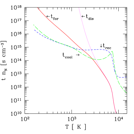
Figure 4: Evolution of the time scales in the steady flow calculation are presented. The initial shock velocity is $100\;{\rm km/s}$. The solid line, dotted line, short-dashed line and long-dashed line represent $t_{\rm for},t_{\rm dis},t_{\rm rec}$ and $t_{\rm cool}$, respectively. Every time scale is multiplied by density.

The numerically calculated evolutionary path of $y_{\rm H_{2}}$ is presented in Fig. 2. The chemical equilibrium for the hydrogen molecule holds outside of the shaded region in the $y_{e}$-$T$ plane. Once the system comes into the shaded region, the fraction of ${\rm H_{2}}$ departs from the chemical equilibrium and eventually freezes to a certain value, because the cooling proceeds faster than the dissociation and formation of hydrogen molecules.

The evolution of the time scales in numerical calculation ($v_{s}=100\;{\rm km/s}$) is presented in Fig. 4. The dissociation time scale is identical to the formation time scale for $T\mathrel{\mathchoice{\lower 2.15277pt\vbox{\halign{$\mathsurround 0pt \displaystyle\hfil#\hfil$\cr>\crcr\sim\crcr}}}{\lower 2.15277pt\vbox{\halign{$\mathsurround 0pt \textstyle\hfil#\hfil$\cr>\crcr\sim\crcr}}}{\lower 2.15277pt\vbox{\halign{$\mathsurround 0pt \scriptstyle\hfil#\hfil$\cr>\crcr\sim\crcr}}}{\lower 2.15277pt\vbox{\halign{$\mathsurround 0pt \scriptscriptstyle\hfil#\hfil$\cr>\crcr\sim\crcr}}}}\;4000{\rm K}$, and they are smaller than the cooling time. For $T\mathrel{\mathchoice{\lower 2.15277pt\vbox{\halign{$\mathsurround 0pt \displaystyle\hfil#\hfil$\cr<\crcr\sim\crcr}}}{\lower 2.15277pt\vbox{\halign{$\mathsurround 0pt \textstyle\hfil#\hfil$\cr<\crcr\sim\crcr}}}{\lower 2.15277pt\vbox{\halign{$\mathsurround 0pt \scriptstyle\hfil#\hfil$\cr<\crcr\sim\crcr}}}{\lower 2.15277pt\vbox{\halign{$\mathsurround 0pt \scriptscriptstyle\hfil#\hfil$\cr<\crcr\sim\crcr}}}}\;4000{\rm K}$, $t_{\rm dis}$ becomes larger than $t_{\rm cool}$, and $y_{\rm H_{2}}$ starts to depart from $y_{\rm H_{2}}^{eq}$. At a slightly lower temperature, $t_{\rm for}$ also becomes larger than $t_{\rm cool}$. As a result, the value of $y_{\rm H_{2}}$ approximately freeze for $T\mathrel{\mathchoice{\lower 2.15277pt\vbox{\halign{$\mathsurround 0pt \displaystyle\hfil#\hfil$\cr<\crcr\sim\crcr}}}{\lower 2.15277pt\vbox{\halign{$\mathsurround 0pt \textstyle\hfil#\hfil$\cr<\crcr\sim\crcr}}}{\lower 2.15277pt\vbox{\halign{$\mathsurround 0pt \scriptstyle\hfil#\hfil$\cr<\crcr\sim\crcr}}}{\lower 2.15277pt\vbox{\halign{$\mathsurround 0pt \scriptscriptstyle\hfil#\hfil$\cr<\crcr\sim\crcr}}}}\;4000{\rm K}$. The final value of $y_{\rm H_{2}}$ is $10^{-3}$ for $v_{s}\mathrel{\mathchoice{\lower 2.15277pt\vbox{\halign{$\mathsurround 0pt \displaystyle\hfil#\hfil$\cr>\crcr\sim\crcr}}}{\lower 2.15277pt\vbox{\halign{$\mathsurround 0pt \textstyle\hfil#\hfil$\cr>\crcr\sim\crcr}}}{\lower 2.15277pt\vbox{\halign{$\mathsurround 0pt \scriptstyle\hfil#\hfil$\cr>\crcr\sim\crcr}}}{\lower 2.15277pt\vbox{\halign{$\mathsurround 0pt \scriptscriptstyle\hfil#\hfil$\cr>\crcr\sim\crcr}}}}30\;{\rm km/s}$, and smaller for slower shock velocities. The frozen values degenerate for faster shock velocities, because the ionization degrees also degenerate for $v_{s}\mathrel{\mathchoice{\lower 2.15277pt\vbox{\halign{$\mathsurround 0pt \displaystyle\hfil#\hfil$\cr>\crcr\sim\crcr}}}{\lower 2.15277pt\vbox{\halign{$\mathsurround 0pt \textstyle\hfil#\hfil$\cr>\crcr\sim\crcr}}}{\lower 2.15277pt\vbox{\halign{$\mathsurround 0pt \scriptstyle\hfil#\hfil$\cr>\crcr\sim\crcr}}}{\lower 2.15277pt\vbox{\halign{$\mathsurround 0pt \scriptscriptstyle\hfil#\hfil$\cr>\crcr\sim\crcr}}}}30\;{\rm km/s}$.

4 Conclusion and discussion

In this paper, we investigated the thermal evolution of the postshock layer in primordial gas clouds. Because of the delay of the recombination process compared to the line cooling due to the hydrogen molecules, significant amounts of electrons ($y_{e}\sim 10^{-3}$) remain below $8000\;{\rm K}$. Feeded the electrons, ${\rm H_{2}}$ also maintains high abundance ($y_{\rm H_{2}}\sim 10^{-3}$) for $T\mathrel{\mathchoice{\lower 2.15277pt\vbox{\halign{$\mathsurround 0pt \displaystyle\hfil#\hfil$\cr<\crcr\sim\crcr}}}{\lower 2.15277pt\vbox{\halign{$\mathsurround 0pt \textstyle\hfil#\hfil$\cr<\crcr\sim\crcr}}}{\lower 2.15277pt\vbox{\halign{$\mathsurround 0pt \scriptstyle\hfil#\hfil$\cr<\crcr\sim\crcr}}}{\lower 2.15277pt\vbox{\halign{$\mathsurround 0pt \scriptscriptstyle\hfil#\hfil$\cr<\crcr\sim\crcr}}}}several\times 10^{3}\;{\rm K}$, then the cloud temperature drops to $T\sim 100\;{\rm K}$ quickly due to the ${\rm H_{2}}$ line cooling. We have shown that both of the residual values of $y_{e}$ and $y_{\rm H_{2}}$ are universal for $v_{s}\mathrel{\mathchoice{\lower 2.15277pt\vbox{\halign{$\mathsurround 0pt \displaystyle\hfil#\hfil$\cr>\crcr\sim\crcr}}}{\lower 2.15277pt\vbox{\halign{$\mathsurround 0pt \textstyle\hfil#\hfil$\cr>\crcr\sim\crcr}}}{\lower 2.15277pt\vbox{\halign{$\mathsurround 0pt \scriptstyle\hfil#\hfil$\cr>\crcr\sim\crcr}}}{\lower 2.15277pt\vbox{\halign{$\mathsurround 0pt \scriptscriptstyle\hfil#\hfil$\cr>\crcr\sim\crcr}}}}30\;{\rm km/s}$ by simple comparison of time scales. The universality of the values to which $y_{e}$ and $y_{\rm H_{2}}$ converge is explained as follows: The evolution of the system is basically determined by $T$, $y_{e}$ and $y_{\rm H_{2}}$. However, at high temperature, $y_{\rm H_{2}}$ attains its equilibrium value, and at low temperature, it will freeze to a value, because cooling precedes the dissociation and the formation of hydrogen molecules. Therefore the evolution of the system is predicted just by $T$ and $y_{e}$. The convergence of $y_{e}$ and $y_{\rm H_{2}}$ occurs when the coolant changes from hydrogen atoms to hydrogen molecules. In fact, assuming an isobaric cooling time, the predicted evolutionary paths agree very well with the numerically integrated paths for steady flow.

These results are not restricted to the case of steady postshock flow, and what is more, the shock diagram describes not only the evolution of the postshock flow but also the primordial gas cloud which is once heated up to $10^{4}\;{\rm K}$. The argument in §2 simply depends on the comparison of time scales. When we compare the shock diagram (Fig. 1) with the numerically integrated results, the steadiness of the flow is used just as the isobaricity of the postshock flow in Eq. (3), by choosing $C_{p}$. However, even if we choose $C_{v}$ in Eq. (3), $t_{\rm cool}$ is not much different from the cooling time for the isobaric flow. We have

$$\frac{t_{\rm cool}^{\rm isobaric}}{t_{\rm cool}^{\rm isochoric}} = C_{p}/C_{v},$$ (12)

$$= \gamma.$$ (13)

Consequently, the $y_{e}$-$T$ diagram obtained for the isochoric case, is very similar to Fig. 1. The diagram for the isochoric case is presented in Fig. 5. It is obvious that the difference between Fig. 1 and Fig. 5 is small. In the isochoric case, the final fraction of hydrogen molecules is $\sim 10^{-3}$ again, as in the isobaric case. Hence, the intermediate case should have a similar diagram.

Figure 5: Same as Fig. 1, except that the cooling time is estimated by assuming the isochoric evolution of the cloud.

Furthermore, the shock diagrams are applied not only to the postshock flow but also to primordial gas clouds which are initially sufficiently heated ($T\mathrel{\mathchoice{\lower 2.15277pt\vbox{\halign{$\mathsurround 0pt \displaystyle\hfil#\hfil$\cr>\crcr\sim\crcr}}}{\lower 2.15277pt\vbox{\halign{$\mathsurround 0pt \textstyle\hfil#\hfil$\cr>\crcr\sim\crcr}}}{\lower 2.15277pt\vbox{\halign{$\mathsurround 0pt \scriptstyle\hfil#\hfil$\cr>\crcr\sim\crcr}}}{\lower 2.15277pt\vbox{\halign{$\mathsurround 0pt \scriptscriptstyle\hfil#\hfil$\cr>\crcr\sim\crcr}}}}10^{4}\;{\rm K}$ ).

Hence the argument in the previous paragraph implies that the thermal evolution of the primordial gas cloud is determined by the “shock diagram”, unless the system becomes gravitationally unstable or some processes originating from external radiation fields become important. The dynamical evolution of the system is roughly determined by the sound crossing time $t_{\rm sc}$, free fall time $t_{\rm ff}$, and $t_{\rm cool}$. In the case that $t_{\rm sc}$ is the shortest time scale, the evolution of the system is nearly isobaric, and in the case that $t_{\rm cool}$ is the shortest, the evolution is approximately isochoric. In both cases, we can apply the shock diagrams on the thermal evolution of the system. In the third case, when $t_{\rm ff}$ is the shortest, the evolution is different from both of the above two cases. However, in a realistic situation, such as the shocks in dynamically collapsing primordial gas clouds, at first the isobaric case is realized generally, as discussed by Yamada and Nishi.[30] Results of numerical simulations also imply that the shock diagrams can be applied in this situation. In fact, in dynamically collapsing primordial gas clouds, hydrogen molecules are formed up to $y_{\rm H_{2}}\sim 10^{-3}$, [1, 28] though the gas is not always isobaric because of a non-steady state of the shock wave.

The gravitational instability of sheets may change the thermal evolution of the primordial gas from the predicted path in the shock diagram. The shocked and compressed layer may fragment into small pieces with a roughly local free-fall time which is proportional to $\rho^{-1/2}$ (Ref. ElEl). In steady shock waves, Yamada and Nishi[30] discussed this problem by comparing the time scale of fragmentation and the cooling time.

The external UV radiation field, which exists at the early epoch of the universe, may affect the thermal evolution of pregalactic gas. The reaction rates of photoionization process and photodissociation process have different dependence on density from the other reactions induced by collision. As a result, the above arguments based on Figs. 1 and 5 are changed significantly. However, the external UV radiation field does not exist, as long as we are interested in the first objects in the universe.

Consequently, once the primordial gas cloud is heated above $10^{4}\;{\rm K}$ and there is no external radiation field, significant amounts of hydrogen molecules are formed ($y_{\rm H_{2}}\sim 10^{-3}$), and the temperature drops much below $10^{4}\;{\rm K}$, until some other time scales become comparable to the thermal and chemical time scales.

Appendix A Reactions

We include the following reactions to obtain the dynamical evolution of the postshock layer in §3. The reaction rates are given in the listed reference in the Table 1.

Table 1: Reaction rates

Reactions	References
H++ e $\rightarrow$H + $\gamma$	Spitzer 1956 [25]
H + e $\rightarrow$H-+ $\gamma$	de Jong 1972 [4]
H-+ H $\rightarrow$H2+e	Beiniek 1980 [2]
3H $\rightarrow$H2+ H	Palla, Salpeter & Stahler 1983 [17]
H2+ H $\rightarrow$3H	SK [23]
2H + H2$\rightarrow$2H2	Palla, Salpeter & Stahler 1983[17]
2H2$\rightarrow$2H + H2	SK [23]
H + e $\rightarrow$H++2e	Lotz 1968 [13]
2H $\rightarrow$H + H++ e	Palla, Salpeter & Stahler 1983 [17]
H + H+$\rightarrow$H${}_{2}^{+}$+ $\gamma$	Ramaker & Peek 1976 [21]
H${}_{2}^{+}$+ H $\rightarrow$H2+ H+	Karpas, Anicich & Huntress 1979 [11]
H2+ H+$\rightarrow$H${}_{2}^{+}$+ H	Prasad & Huntress 1980 [19]
H-+ H+$\rightarrow$H${}_{2}^{+}$+ e	Poularert et.al. 1978 [18]
H${}_{2}^{+}$+ e $\rightarrow$2H	Mitchell & Deveau 1983 [16]
H${}_{2}^{+}$+ H-$\rightarrow$H + H2	Prasad & Huntress 1980 [19]
H-+ e $\rightarrow$H + 2e	Duley 1984 [5]
H-+ H $\rightarrow$2H + e	Izotov & Kolensnik 1984 [8]
H-+ H+$\rightarrow$2H	Duley 1984 [5]

Appendix B Steady Shock

In this appendix, the basic equations of the steady shock are presented. The numerical results presented in §3 are based on the following equations. SK solved these equations coupled with the chemical reactions. One of the most important features of the steady shock is the approximate isobaricity of the postshock layer.

B.1 Basic equations

The jump conditions at the shock front are

$$\rho_{1}v_{1} = \rho_{2}v_{2},$$ (14)

$$\rho_{1}v_{1}^{2}+p_{1} = \rho_{2}v_{2}^{2}+p_{2},$$ (15)

$$v_{1}\left(\frac{\rho_{1}v_{1}^{2}}{2}+\frac{\gamma_{1}}{\gamma_{1}-1}p_{1}\right) = u_{2}\left(\frac{\rho_{2}v_{2}^{2}}{2}+\frac{\gamma_{2}}{\gamma_{2}-1}p_{2}\right).$$ (16)

These equations constitute the conservation law of the mass, momentum and energy across the shock front. The quantities whose suffixes are 1 and 2 denote the hydrodynamical variable in the preshock region and the postshock region, respectively. In case that the shock is strong, i.e. the sound velocity in the preshock region is much smaller than the bulk velocity $u_{1}$, we obtain from Eqs. (14)$\sim$(16),

$$\rho_{2}/\rho_{1} = v_{1}/v_{2}=4,$$ (17)

$$kT = \frac{3}{16}\mu m_{p}v_{1}^{2},$$ (18)

where $\mu$ and $m_{p}$ are the mean molecular weight of the gas and proton mass.

Behind the shock front, the assumption that the flow is steady allows us to write the conservation of mass, momentum and the energy as

$$\rho v = \rho_{2}v_{2},$$ (19)

$$\rho v^{2}+p = \rho_{2}v_{2}^{2}+p_{2},$$ (20)

$$\frac{dE}{dt} = (\Gamma-\Lambda)+[(p+E)]\frac{1}{\rho}\frac{d\rho}{dt},$$ (21)

where $\Gamma$, $\Lambda$ and $E$ denote the heating and cooling rates, and the internal energy per unit volume, and $d/dt$ is the Lagrange derivative. The hydrodynamical variables with no suffix denote quantities at a general point behind the shock front. In addition, we require the equation of state $p=nkT$. Then the equations are closed, and we can solve the flow equations.

B.2 Isobaricity of the postshock layer

The assumption that the flow is steady indicates the approximate isobaricity of the postshock region (Ref. YN). From Eqs. (20) and (21) and the equation of state, $p=\rho kT/(m_{p}\mu)$, the relative compression factor $x\equiv\rho/\rho_{2}$ is given by

$$\frac{kT}{m_{p}\mu}x^{2}-(1+\frac{p_{2}}{\rho_{2}v_{2}^{2}})x+v_{2}^{2}=0.$$ (22)

In case the shock is strong, the above equation becomes

$$\frac{kT}{m_{p}\mu}x^{2}-4v_{2}^{2}x+v_{2}^{2}=0.$$ (23)

Its solution exists if the condition

$$v_{2}^{2}(4v_{2}^{2}-\frac{kT}{m_{p}\mu})\geq 0$$ (24)

is satisfied, and this condition holds unless the heating rate is not too high to raise the temperature by a factor of $4/3$ in the postshock flow.

The solution is expressed as

$$x=\frac{m_{p}\mu}{kT}v_{2}^{2}\left(2+\sqrt{4-\frac{kT}{m_{p}\mu v_{2}^{2}}}\right).$$ (25)

If we define $T_{2}$ as

$$kT_{2} = 3\mu m_{p}v_{2}^{2},$$ (26)

the pressure $p$ can be written as follows:

$$p=\frac{2}{3}p_{2}\left(1+\sqrt{1-\frac{3}{4}\frac{T}{T_{2}}}\right).$$ (27)

Thus, $p/p_{2}$ can be determined by $T/T_{2}$ only, and the dependence is weak.

After the gas has cooled down to $T\ll T_{2}$, $p$ has the asymptotic value, $4/3p_{2}$, which is not much different from $p_{2}$. As a result, the postshock region is almost isobaric for a wide range of temperatures.

References

- [1] P. Anninos and M.J. Norman, Astrophys.J., 460(1996), 556.
- [2] R.J. Beiniek, J.Phys.B, 13(1980), 4405.
- [3] R.G. Carlberg, Mon.Not R. Astron. Soc., 197(1981), 1021.
- [4] T. de Jong, Astron and Astrophys., 20(1972), 263.
- [5] W.W. Duley and D.A. Williams, 1984, Interstellar Chemistry (London:Academic Press).
- [6] B.G. Elmegreen and D.M. Elmegreen, Astrophys.J., 220(1978), 1051.
- [7] D. Hollenbach and C. McKee, Astrophys.J. Suppl., 41(1979), 55.
- [8] Yu.I. Izotov and I.G. Kolensnik, Soviet Astro., 28(1984), No. 1, 15.
- [9] O. Lahav, Mon.Not R. Astron. Soc., 220(1986), 259.
- [10] H. Kang and P.R. Shapiro, Astrophys.J., 386(1992), 432.
- [11] Z. Karpas, V. AAnicich, and W.T.,Jr. Huntress, J.Chem.Phys., 70(1979), No.6, 2877.
- [12] S. Lepp and J.M. Shull, Astrophys.J., 270(1983), 578.
- [13] W. Lotz, Zs.Phys., 216(1968), 241.
- [14] M.M. MacLow and J.M. Shull, Astrophys.J., 302(1986),585.
- [15] T. Matsuda, H. Sato and H. Takeda, Progr.Theor.Phys., 42(1969), 219.
- [16] G.F. Mitchell and T.J. Deveau, Astrophys.J., 266(1983), 646.
- [17] F. Palla,E.E. Salpeter and S.W. Stahler, Astrophys.J., 271(1983),632.
- [18] G. Poularert, F. Brouillard, W. Claeys, J.W. McGowan, and G. Van Wassenhove, J.phys., B, 11(1978), L671.
- [19] S.S. Prasad and W.T.,Jr. Huntress, Astrophys.J.Suppl.(1980), 43,1.
- [20] D. Puy and M. Signore, Astron and Astrophys., 305(1996), 371.
- [21] D.E. Ramaker, and J.M. Peek, Phys.Rev. A, 13(1976), 58.
- [22] M.J. Rees and J.P. Ostriker, Mon.Not R. Astron. Soc., 179(1977), 541.
- [23] P.R. Shapiro and H. Kang, Astrophys.J., 318(1987), 32.
- [24] J. Silk, Astrophys.J., 214(1977), 152.
- [25] L. Jr. Spitzer, 1956, The Physics of Fully ionized Gases(New York:Interscience), p.88.
- [26] C. Struck-Marcell, Astrophys.J., 259(1982), 116.
- [27] C. Struck-Marcell, Astrophys.J., 259(1982), 127.
- [28] H. Susa, 1997, Thesis “The thermal evolution of primordial gas clouds : A clue to galaxy formation”, Kyoto University, Japan.
- [29] H. Susa, H. Uehara, and R. Nishi, Progr. Theor. Phys., 96(1996), 1073.
- [30] M. Yamada and R. Nishi 1997, submitted to Astrophys.J..