Fast maximum entropy Doppler mapping
H.C. Spruit
Max Planck Institut für Astrophysik, Box 1523, D-85740 Garching
henk@mpa-garching.mpg.de
Abstract A numerical code is described for constructing Doppler maps from the orbital variation of line profiles of (mass transfering) binaries. It uses an algorithm related to Richardson-Lucy iteration, and is much faster than the standard algorithm used for ME problems. The method has been tested on data of cataclysmic variables (including WZ Sge and SS Cyg), producing maps of up to 300X300 points. It includes an IDL-based set of routines for manipulating and plotting the input and output data, and can be downloaded from http://www.mpa-garching.mpg.de/henk.
Introduction
The orbital variation of spectral line profiles in a binary contains information on the distribution of emitting or absorbing regions in the system. The process of Doppler mapping (Horne and Marsh, 1988) converts the orbital-phase dependent line profile into a map in velocity space. This map is easier to interpret than the original line profile. If the relation between velocity and position is known, for example if the binary parameters are known and/or the velocities in the accretion disk are assumed to be Keplerian, this can then be used to derive information on the spatial distribution of emitting material.
Doppler mapping has become a standard tool for work on Cataclysmic Variables and X-ray binaries (e.g. Horne 1991, McClintock et al. 1995, Marsh and Duck 1996, Harlaftis et al. 1996, 1997, Schwope et al. 1997, Steeghs et al. 1997). Most commonly used is some form of Fourier-filtered back-projection, which is easy to implement and fast. It tends to produce noticeable artefacts, however, in the form of ‘radial spokes’. Much cleaner results are obtained with a Maximum Entropy procedure (Marsh and Horne 1988). Standard implementations of this method, however, are so slow that only rather small maps can be conveniently processed (interactively, say) on current workstations.
The algorithm implemented here solves the same maximum entropy problem, but with a very much faster algorithm. Technically, it derives from the Richardson-Lucy maximum-likelihood algorithm, but solves a different problem. Its efficiency has been demonstrated before in the case of eclipse mapping (Spruit 1994). The code described here has been used by Spruit and Rutten (1998) for Doppler mapping of WZ Sge.
Method
The formulation of the Doppler mapping (or Doppler tomography) problem has been described in detail in Marsh and Horne (1988). In brief, it is assumed that the system consists of optically thin emission regions, and that the emission is stationary in a frame corotating with the orbit. The line-of-sight velocity of each element of emitting material then varies sinusoidally with the orbital phase. The line profile at each orbital phase is then a superposition a large number of these sinusoidally varying line profiles. In most systems, the line profile in the rest frame of the gas is fairly narrow compared with the velocity of the gas, and is usually neglected campared with the Doppler shifts due to motion.
The code described here assumes, finally, that all the emission takes place in a single plane, the orbital plane of the system. This is appropriate if the accretion disk is the main object of study. In principle, however, an arbitrary geometry of the emitting surfaces can be included as long as it can be specified in advance. An example is the Roche lobe mapping of Rutten and Dhillon (1994).
Take cartesian coordinates in the space describing the velocity of material in the orbital plane . Discretize this velocity space in bins of size and number these points (in some fixed but arbitrary order) . Let each of these bins have an emissivity (per unit of velocity2) , the Doppler map. This distribution of emission in velocity space produces a phase-dependent line profile , where is the line of sight velocity and the orbital phase. Let be discretized in points (again in arbitrary but fixed order). Then the transformation from the emission distribution in velocity space to the line profile is given by a linear matrix operator :
| (1) |
The form of has been described in the previous literature cited. Let the observed spectrum be . The object of the reconstruction process is now to determine a Doppler map such that matches within the observational uncertainties while making as few assumptions on the nature of the map as possible. In the ‘maximum entropy’ formulation, this becomes an optimization problem in which a single scalar quantity (‘quality function’ or ‘energy’) is maximized:
| (2) |
where , the likelihood, is a number which maximizes when the observations are matched exactly (), and , the entropy, maximizes for ‘smooth’ maps. For the likelihood, two forms are in current use, the logarithmic one advocated by Lucy for positive definite images:
| (3) |
and a -based likelihood:
| (4) |
For the entropy, we use the form with ‘floating defaults’ introduced by Horne (1985):
| (5) |
where is a default image created from the map by a smearing operation. For this smearing we use a simple Gaussian smearing in velocity space with an adjustable width. The purpose of this default is to bias the resulting map to a ‘smooth’ map without necessarily biasing it toward a completely flat one. This has become standard practice in eclipse mapping and Doppler mapping applications.
The value of regulates how close a fit to the input data is obtained. An objective measure would be to choose such that the reconstructed spectrum fits the input data just within the error bars but not closer. In practice, there are always features in the input data that can not be fitted at all because the assumptions made (in particular the optically thin nature of the emission) are violated by the data. A compromise then has to be made, based in part on personal judgement.
The optimization is done iteratively by adjusting the values of . The iteration is a slightly modified version of that of Lucy (1994), and is described in detail in Spruit (1994). It converges to a single unique maximum in 20-40 iterations, each of which uses 3 forward and 1 backward projections.
Computing resources
The computations are done in double precision. The projection matrix accounts for almost all of the memory used by the code. For efficient access, it has to be stored along with its transpose. It can, however, be stored in single precision without loss of accuracy. Since most of the elements of vanish, index arrays are used to map the indices of the nonvanishing elemnts into linear arrays. This adds an equal amount of storage in the form of long integers, so that the total storage is 8 bytes per nonvanishing element of the matrix.
Let be the number of wavelength points of the spectra and the number of orbital phases (number of spectra). Let be the number of points in each of the two velocity coordinates in the Doppler map. If the resolution in the Doppler map is matched to the wavelength resolution of the spectra, . In this case both the computing time and the amount of main memory used scale as , more or less independent of . For a map of 80X80 points, produced from 160 spectra of 80 wavelength points, the cpu time is of the order 30s, and 45 MB of memory are needed. The largest map on which the code was tested (from high resolution data of SS Cyg in quiescence) has , . On the order of 15 minutes and 1.5 GB were used.
Examples
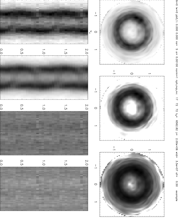
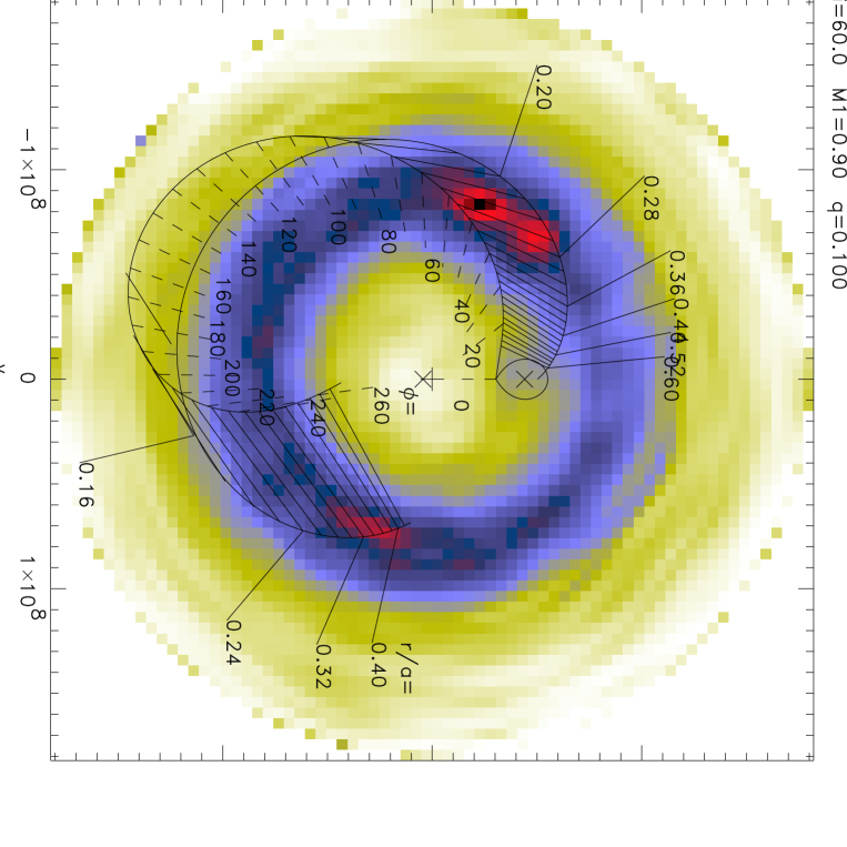
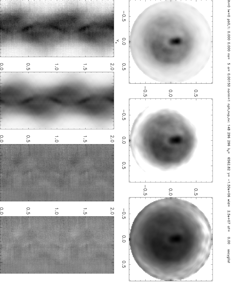
Fig. 1 shows the postscript output produced from a dataset consisting of 17 spectra of 72 wavelength points. The lack of resolution in the azimuthal direction due to the rather low number of phase points is evident. Figure 2 shows the same Doppler map with mass transfering stream and secondary star overplotted. Figure 3 shows the results from high resolution spectra of SS Cyg in quiescence. Spectral resolution was 0.24Å (two pixels per resolution element), phase resolution 0.01.
downloading the software
The package can be accessed by web browser athttp://www.mpa-garching.mpg.de/henk. It has been extensively tested on IBM AIX, HP/UX and Sun Solaris machines, and I consider it stable. When publishing results in which use has been made of this package, please acknowledge this by a reference to the present publication. Bug reports are welcome. The package includes a documentation text, sample input spectra, sample output data and and ps files from the graphics routines.
The actual Doppler mapping is done by a Fortran 77 program that can be used stand-alone. Recommended use however is with the set of IDL routines provided. Apart from plotting results and input data, they are designed to simplify running of the Fortran code.
Acknowledgements
I thank Drs. Keith Horne and Leon Lucy for discussions on various aspects of astromical image reconstruction problems.
References
- [1] Harlaftis E.T., Steeghs D., Horne K., Filipenko A.V., 1997, AJ 114, 1170
- [2] Harlaftis E.T., Horne K., Filipenko A.V., 1996 PASP 108, 762
- [3] Horne, K., 1985, MNRAS 213,129
- [4] Horne, K., 1991, in Fundamental properties of Cataclysmic Variable stars, ed. A.W. Shafter, Dept of Astronomy, San Diego State University, p.23
- [5] Lucy L.B., 1994, A&A 289, 983
- [6] Marsh T.R., Duck S.R., 1996, New Astron. 1, 97
- [7] Marsh T.R., Horne, K., 1988, MNRAS 235, 269
- [8] McClintock J.E., Horne K., Remilliard R.A., 1995, ApJ 442, 358
- [9] Rutten R.G.M., Dhillon V.S., 1994 A&A 288, 773
- [10] Schwope A.D., Mantel K.-H., Horne K., 1997, A&A 319, 894
- [11] Spruit H.C., 1994, A&A 289, 441
- [12] Spruit H.C., Rutten R.G.M., 1998, MNRAS, in press
- [13] Steeghs D., Harlaftis E.T., Horne K., 1997, MNRAS 290, 28. erratum in MNRAS 296, 463