Lensing and high-$z$ supernova surveys

Abstract

Gravitational lensing causes the distribution of observed brightnesses of standard candles at a given redshift to be highly non-gaussian. The distribution is strongly, and asymmetrically, peaked at a value less than the expected value in a homogeneous Robertson-Walker universe. Therefore, given any small sample of observations in an inhomogeneous universe, the most likely observed luminosity is at flux values less than the Robertson-Walker value. This paper explores the impact of this systematic error due to lensing upon surveys predicated on measuring standard candle brightnesses. We re-analyze recent results from the high-$z$ supernova team (Riess et al. 1998a ), both when most of the matter in the universe is in the form of compact objects (represented by the empty-beam expression, corresponding to the maximal case of lensing), and when the matter is continuously distributed in galaxies. We find that the best-fit model remains unchanged (at $\Omega_{m}=0$, $\Omega_{\Lambda}=0.45$), but the confidence contours change size and shape, becoming larger (and thus allowing a broader range of parameter space) and dropping towards higher values of matter density, $\Omega_{m}$ (or correspondingly, lower values of the cosmological constant, $\Omega_{\Lambda}$). These effects are slight when the matter is continuously distributed. However, the effects become considerably more important if most of the matter is in compact objects. For example, neglecting lensing, the $\Omega_{m}=0.5$, $\Omega_{\Lambda}=0.5$ model is more than $2\sigma$ away from the best fit. In the empty-beam analysis, this cosmology is at $1\sigma$.

1 INTRODUCTION

Recently there has been great activity in determining cosmological parameters based on the observations of type Ia supernovae at high redshifts (Perlmutter et al. (1998), 1997; Riess et al. 1998a ; Schmidt et al. (1998)). The peak flux of these supernovae is thought to be known to within $0.15\ \mbox{mag}$ (Hamuy et al. (1996); Riess, Press, & Kirshner (1996)), making them excellent standard candles with which to measure the luminosity distance–redshift relation. As this relation is dependent upon the cosmological parameters ($H_{0}$, $\Omega_{m}$, $\Omega_{\Lambda}$), it is possible to infer the values of these parameters from supernova Ia observations. Two independent groups (Perlmutter et al. (1998); Schmidt et al. (1998)) have been pursuing cosmology via supernova surveys, and preliminary results argue for a low mass density (Perlmutter et al. (1998); Schmidt et al. (1998)), and a nonzero cosmological constant (Riess et al. 1998a ).

The apparent brightness of a standard candle, at a given redshift, is a function not only of the Robertson-Walker model describing the universe, but also of the distribution of matter within the universe. To date, the cosmology results in the literature derived from observed supernova peak brightnesses are based upon the assumption that the matter in the universe is homogeneously distributed. An important question is to what extent the matter inhomogeneities we see (in the form of galaxies, stars, MACHOs, etc.) affect one’s ability to draw conclusions from the data.

It is well known that weak gravitational lensing can impact the degree to which high-redshift supernovae can be considered standard candles, contributing “errors” on the order of $0.05\ \mbox{mag}$ by redshift of one for various cosmologies (Kantowski, Vaughan, & Branch (1995); Frieman (1997); Wambsganss, Cen, Xu, & Ostriker (1998); Holz & Wald (1998); Kantowski 1998a , 1998b). These errors can be beaten down through statistics, since, given a large enough sample of supernovae at a given redshift, the average flux of the supernovae should be representative of the true flux in a pure Robertson-Walker universe. Work has also been done analyzing the high-magnification tail of the lensing distribution, and the information this yields about the distribution of mass inhomogeneities (Schneider & Wagoner (1987)). In contrast, the present paper examines the low-magnification part of the lensing distribution, and explores the systematic errors due to the non-gaussian peak. A similar study has been undertaken by Kantowski (1998a, 1998b), examining fits to analytic distance–redshift relations from Swiss-Cheese model universes. In this paper we utilize a newly-developed model to determine lensing statistics (Holz & Wald (1998)). With this model we are able to re-analyze current results from supernova surveys, both in the case of the maximal (empty-beam) lensing effects, and in the case where matter is distributed continuously in galaxies.

2 DISTANCE–REDSHIFT RELATIONS

The luminosity of an image, as a function of redshift, is related to the angular diameter distance to the source generating the image. Two common angular diameter distance–redshift relations are given by the filled and empty-beam expressions (Dyer & Roeder (1972), 1973; Fukugita et al. (1992)), where in the filled-beam case the line-of-sight to the source traverses mass of exactly the Robertson-Walker density, while in the empty-beam case the beam encounters no curvature (i.e., passes through vacuum, far from all matter distributions). Current analyses of high-$z$ supernova data use filled-beam expressions to infer the physical distances of the sources from their observed apparent brightnesses (Perlmutter et al. (1998); Riess et al. 1998a ). When calculating how far a source is, based upon the brightness of its image, it is therefore assumed that the photon beams pass through exactly the Robertson-Walker mass density. If, for example, the photon beams avoid most of the matter, then a more accurate description would be the empty-beam expressions. By assuming a filled-beam expression in this case, one takes an image dimmed because of the lack of matter in the beam, and concludes from the observed brightness of this image that the source is further away than it really is. With increasing redshift, the differences between the filled and empty-beam brightnesses increase. In this way, evidence of an inhomogeneous universe might be mistaken for evidence of an accelerating one.

The filled and empty-beam distance–redshift relations reduce to the same form for low $z$, and thus measurements of cosmological parameters from supernovae with statistical weight at lower redshifts will not be affected by lensing. As one moves to higher redshifts, however, the differences between the two expressions can be dramatic. For example, at $z=1$ a standard candle described by the filled-beam expression in a smooth Robertson-Walker universe, with $\Omega_{m}=0.5$, $\Omega_{\Lambda}=0.5$, will have the same apparent brightness as a standard candle described by the empty-beam expression in an inhomogeneous universe, with $\Omega_{m}=0.5$, $\Omega_{\Lambda}=0$. Therefore, based solely upon observations of standard candles at both low redshifts and at a single high redshift, it would be impossible to conclude whether dimming was due to lensing effects or a nonzero cosmological constant. Knowledge of the distance–redshift curve at a range of intermediate to high redshifts is thus crucial.

3 MAGNIFICATION DISTRIBUTIONS

We generate magnification distributions utilizing a recently-developed method to determine lensing statistics in inhomogeneous universes (Holz & Wald (1998)). In brief, the method arrives at statistical lensing information by combining aspects from ray-tracing and Swiss-Cheese model numerical approaches. The universe is decomposed into comoving spherical regions, with arbitrary mass inhomogeneities allowed within each region. Statistics are developed by considering many random rays in a Monte-Carlo fashion, and integrating the geodesic deviation equation along each ray in turn. It should be emphasized that this method calculates the lensing effects in full generality, treating both weak and strong lensing effects automatically.

Some representative magnification distributions are shown in Figure 1, for two different matter distributions.

                 

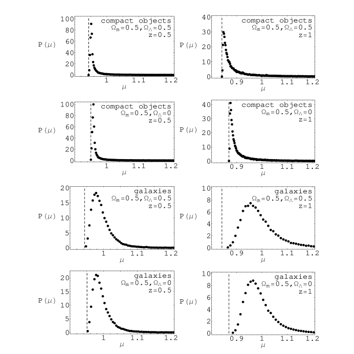
Figure 1: Probability distribution, $P(\mu)$, for supernova apparent brightness, $\mu$, normalized so that $\mu=1$ corresponds to the filled-beam, or homogeneous Robertson-Walker, value. The vertical dashed lines are at the empty-beam value. The brightness distributions are at $z=0.5$ and $z=1$, for the models as indicated. The “compact objects” distribution is for the case where all of the matter is in point masses. The “galaxies” distribution is for matter in isothermal spheres with truncation radii $380\ \mbox{kpc}$.

The “compact objects” panels give the magnification distributions when most of the matter in the universe is in highly condensed (point mass) objects with masses $\!{\mathbin{\lower 3.0pt\hbox{$\,\hbox to0.0pt{\raise 5.0pt\hbox{$\char 62\relax$}\hss}\mathchar 29208\relax\,$}}}0.01\ \mbox{M}_{\odot}$ (stars, MACHOs, etc.). These results are independent of the mass distribution and clustering of the point masses (Holz & Wald (1998)). At the redshifts being considered, point mass lensing will in general be dominated by a single lens encounter, and two images will be generated. The numerical method we utilize generates statistics for uncorrelated photon beams, and thus does not identify the two images associated with a given source (Holz & Wald (1998)). However, using analytic expressions for the relative brightnesses of these images (Schneider, Ehlers, & Falco (1992)), we are able to convert the magnification distribution for the beams that have not passed through a caustic (which correspond to the brighter image of a pair) into a magnification distribution for the combined images. The “compact objects” panels of Figure 1 show this combined magnification distribution.

For continuous matter distributions, as in the case of isothermal galaxies, the incidence of multiple imaging at the redshifts being considered is highly improbable ($<\!\!0.2\%$ at $z=1$ (Holz, Miller, & Quashnock (1998))). In this case strong lensing is unimportant, and weak lensing dominates the results. In the “galaxies” panels of Figure 1, we have taken all of the matter in the universe to be in galaxies, where a galaxy is represented as a truncated isothermal sphere of continuously distributed matter. In this paper we take a galaxy number density of $0.025\,h^{3}\ \mbox{Mpc}^{-3}$ (Geller et al. (1997)), which, for a given cosmology, fixes the mass of the galaxies. For example, taking $\Omega_{m}=0.5$ and $H_{0}=65\ \mbox{km}/\mbox{s}\mbox{\ Mpc}^{-1}$, the mass of the galaxies is fixed at $8.5\times 10^{12}\ \mbox{M}_{\odot}$. If we then take the velocity dispersion of the galaxies to be $220\ \mbox{km}/\mbox{s}$, the physical truncation radius of the isothermal spheres is set at $380\ \mbox{kpc}$.

A key feature of the magnification distributions plotted in Figure 1 is that they are non-gaussian. The average of the distributions is given by the Robertson-Walker (filled-beam) value ($\mu=1$). In all cases, however, the magnification distributions are strongly peaked at values considerably less than this average. Another important characteristic of the distributions is that there is a lower cutoff, given by the empty-beam value, to the possible observed de-magnification. In general, the peak of the magnification distribution will lie somewhere in between the empty and filled-beam values.

With good statistics it may become possible to measure the magnification distribution of the supernovae from observations, and thus determine the matter distribution (Metcalf (1998); Wiegert & Frieman (1998)). In the case of low statistics, as is found in the high-$z$ supernova surveys, the likelihood of evenly sampling the probability distribution is low. One therefore would expect these surveys to find a “mean” in rough agreement with the (de-magnified) peak of the distribution, rather than the average. As the number of data points at a given redshift increases (${\mathbin{\lower 3.0pt\hbox{$\,\hbox to0.0pt{\raise 5.0pt\hbox{$\char 62\relax$}\hss}\mathchar 29208\relax\,$}}}50$), the distribution of the average of the data points approaches a gaussian distribution, centered about the average value of the original distribution. However, for the smaller high-$z$ data samples currently available, the distributions of the averages retain the highly non-gaussian form of the original (single data point) distributions. Therefore, in what follows we take the magnification distributions to be approximated by the peaks of the single data point distributions. In the case of compact objects, the distributions are sharply peaked very near the empty-beam limits, and therefore the empty-beam values are excellent approximations to the magnification distributions. For continuous matter distributions, such as extended galactic structures, the peaks of the distributions are still considerably de-magnified from the filled-beam value: The peak always falls in between the empty and filled-beam values. Therefore, in the case of extended matter distributions, doing an analysis with the empty-beam expressions in addition to the filled-beam ones serves to bracket the possible range of lensing effects. In the following section we analyze a sample high-$z$ supernova data, fitting to both the empty-beam distance-redshift relation and the peaks of the “galaxies” magnification distributions, as well as the more traditional filled-beam distance-redshift relations.

4 APPLICATION TO SUPERNOVA DATA

We use a sample of supernovae as a test bed to determine the qualitative effects of lensing on high-$z$ supernova surveys. To this end, we take distance data for a total of 37 supernovae from the high-$z$ supernova team: 27 supernovae at $0.01{\,\mathbin{\lower 3.0pt\hbox{$\,\hbox to0.0pt{\raise 5.0pt\hbox{$\char 60\relax$}\hss}\mathchar 29208\relax\,$}}}z{\,\mathbin{\lower 3.0pt\hbox{$\,\hbox to0.0pt{\raise 5.0pt\hbox{$\char 60\relax$}\hss}\mathchar 29208\relax\,$}}}0.1$ (Hamuy et al. (1996)), and ten higher-redshift supernovae reported in Riess et al. (1998a) (and analyzed using the MLCS method of Riess, Press, & Kirshner (1996)), including SN97ck at $z=0.97$ (Garnavich et al. (1998)).

For the low-redshift sample, we take the distance errors listed in Table 10 of Riess et al. (1998a), and the dispersion in host galaxy redshifts (due to peculiar velocities and other uncertainties) to be $200\ \mbox{km}/\mbox{s}$. For the high-$z$ sample, we take the errors listed in Riess et al. (1998a). We find that the fits are not sensitive to the particular error values, in agreement with Riess et al. (1998a).

We fix the Hubble constant to be $65\ \mbox{km}/\mbox{s}\mbox{\ Mpc}^{-1}$, in accord with the determination of Riess et al. (1998a). As $H_{0}$ is determined from supernovae (or other methods) at low redshifts, gravitational lensing is not expected to affect this result. We stress that all of the results discussed in this paper are independent of the value of $H_{0}$.

In parallel with § 4.1 of Riess et al. (1998a), we do a two parameter ($\Omega_{m}$, $\Omega_{\Lambda}$) minimum $\chi^{2}$ fit, neglecting regions with $\Omega_{m}<0$, and other unphysical regions (“no big bang” regions (Carroll, Press, & Turner (1992))). The residual Hubble-diagram (where the $\Omega_{m}=\Omega_{\Lambda}=0$ magnitudes have been subtracted out) for the data set is shown in Figure 2, plotted against the best-fit (minimum $\chi^{2}$) curve, as well as some fiducial curves for reference.

           

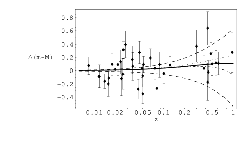
Figure 2: Residual Hubble diagram (the values of the $\Omega_{m}=\Omega_{\Lambda}=0$ model have been subtracted out), with differential distance modulus plotted against redshift, for the supernova data sample and a number of theoretical distance-redshift relations. The top (dashed) curve is for an $\Omega_{m}=0$, $\Omega_{\Lambda}=1$ model. The bottom (dashed) curve is for an $\Omega_{m}=1$, $\Omega_{\Lambda}=0$ model. The dotted curve is the best fit to the data, corresponding to $\Omega_{m}=0$, $\Omega_{\Lambda}=0.45$. The solid curve is the empty-beam distance–redshift relation for $\Omega_{m}=0.4$, $\Omega_{\Lambda}=0.6$. The dot-dashed curve is the filled-beam relation for the same parameters. Note that the empty-beam $\Omega_{m}=0.4$, $\Omega_{\Lambda}=0.6$ case is essentially as good as the best fit ($\chi_{\nu}^{2}=1.17$), while the corresponding filled-beam case is well over $1\sigma$ away ($\chi_{\nu}^{2}=1.24$).

The best fit curve is a model with $\Omega_{m}=0$, $\Omega_{\Lambda}=0.45$ ($\chi_{\nu}^{2}=1.15$, for 35 degrees of freedom). This is in good agreement with the result of Riess et al. (1998a) ($\Omega_{m}=0$, $\Omega_{\Lambda}=0.48$ ($\chi_{\nu}^{2}=1.17$)), which comes from an identical set of supernovae, but with updated MLCS values (Riess et al. 1998b ). Both empty and filled-beam models find this value (which is identical in each case) as their best fit. Note that the data points tend toward values above the axis, indicating a nonzero cosmological constant, regardless of lensing. Also note that the models become most clearly separated at high-$z$, and therefore the discretionary power lies in the few highest-redshift supernovae. This can readily be seen by the striking contrast between contours from Perlmutter et al. (1997) and those from Perlmutter et al. (1998), where the latter paper includes the addition of a single supernova at $z=0.83$. The more sensitive the fits are to the highest-$z$ supernovae, the more lensing effects can come into play.

Although the empty and filled-beam cases agree on a best-fit model, in neither case is the fit particularly tight. Therefore it is particularly informative to consider likelihood contours, as discussed in Riess et al. (1998a). By integrating over successive regions of ($\Omega_{m}$, $\Omega_{\Lambda}$) phase space, we are able to determine the values of $\chi^{2}$ corresponding to the 68%, 95%, and 99.7% confidence boundaries (representing $1\sigma$, $2\sigma$, and $3\sigma$ regions of fit, respectively). Figure 3 shows contours of

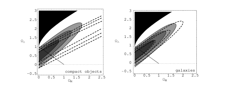
Figure 3: Contours of constant $\chi^{2}$ in ($\Omega_{m}$, $\Omega_{\Lambda}$) parameter space, for the SNe data set of Fig. 2. The background shaded contours correspond to the 68%, 95%, and 99.7% joint confidence intervals in the filled-beam case. The dotted line represents $\Lambda=0$ cosmologies, while the diagonal line represents $\Omega_{m}+\Omega_{\Lambda}=1$ cosmologies. The blackened region at the upper left is excluded (no big bang). The “compact objects” panel includes the confidence intervals (given by the foreground dashed lines) for the empty-beam case. The “galaxies” panel includes the confidence intervals (given by the foreground dashed lines) for the case where matter is assumed to be continuously distributed in isothermal galaxies, and the data is fit to the peaks of the magnification distributions.

constant $\chi^{2}$ representative of these $1\sigma$, $2\sigma$, and $3\sigma$ confidence intervals. In both panels the background shaded contours give the standard filled-beam results. The “compact objects” panel includes the respective contours when the data is fit to empty-beam expressions, corresponding to the maximal lensing case. The “galaxies” panel fits the data to the magnification distributions for isothermal galaxies, of the form shown in Figure 1. It is possible to estimate the value and width of the peaks of these magnification distributions. However, computing a magnification distribution for every point in parameter space, and at each redshift for which there exists data, is numerically prohibitively expensive. For our purposes we have computed magnification distributions for 15 different models, at 4 different redshifts, and interpolated to arrive at peak and width values for the magnification distributions in general. The confidence contours of the “galaxies” panel are for the case where these interpolated peak and width values have been utilized to fit to the data.

All of the contours of Figure 3 are similar near the $\Omega_{m}=0$ axis, where there is little matter to cause lensing. As one progresses to models with more significant matter content, with the matter primarily in the form of compact objects (the empty-beam case), the contours remain wider than their filled-beam counterparts, closing off at much larger $\Omega_{m}$ and $\Omega_{\Lambda}$ values. In this case the inclusion of lensing broadens the class of consistent cosmological models. Furthermore, the empty-beam contours drift downwards: the empty-beam fits prefer higher values of $\Omega_{m}$, and lower values of $\Omega_{\Lambda}$. These results appear to agree with preliminary results from the Supernova Cosmology Project (Aldering (1998)). Although these statements remain true when matter is continuously distributed in galaxies, as can be seen from Figure 3 the effects in this latter case are greatly reduced.

5 CONCLUSIONS

We have argued that lensing will systematically skew the peak of the apparent brightness distribution of supernovae away from the filled-beam value and towards the empty-beam value. Based upon our results from a limited number of supernovae data points, we can make some qualitative statements regarding the impact of this systematic effect on the determination of cosmological parameters from high-$z$ supernova surveys. For universes with little or no $\Omega_{m}$, the effects of lensing are slight. As the current data samples seem to favor vacuum models, lensing will not generally affect their best fits. However, the error ellipses undergo significant changes due to the inclusion of lensing, favoring models with lower values of $\Omega_{\Lambda}$ and higher values of $\Omega_{m}$. If most of the matter in the universe is in the form of compact objects, the effects of lensing can be dramatic. For example, the empty-beam best fit flat model ($\Omega_{m}+\Omega_{\Lambda}=1$) has $\Omega_{m}=0.32$ ($\chi^{2}=1.155$). This fit is essentially as good as the overall best fit ($\Omega_{m}=0$, $\Omega_{\Lambda}=0.45$ ($\chi^{2}=1.152$)). The filled-beam best fit flat model has $\sim\!25\%$ less matter ($\Omega_{m}=0.26$), and is a slightly worse fit ($\chi^{2}=1.161$). If most of the matter is continuously distributed, however, the effects of lensing are greatly reduced.

Currently the true best fit to the data finds negative values for $\Omega_{m}$. As we neglect $\Omega_{m}<0$ on physical grounds, the likelihood contours are squashed up against the $\Omega_{m}=0$ axis, minimizing the effects of lensing. Should future data favor a positive value of $\Omega_{m}$, lensing can be expected to have a greater impact on the analysis.

References

- Aldering (1998) Aldering, G. 1998, private communication
- Carroll, Press, & Turner (1992) Carroll, S. M., Press, W. H., and Turner, E. L. 1992, ARA&A 30, 499
- Dyer & Roeder (1972) Dyer, C.C. & Roeder, R.C. 1972, ApJ, 174, L115
- Dyer & Roeder (1973) ———. 1973, ApJ, 180, L31
- Frieman (1997) Frieman, J. A. 1997, Comments Astrophys., 18, 323; astro-ph/9608068
- Fukugita et al. (1992) Fukugita, M., Futamase, T., Kasai, M., & Turner, E. L. 1992, ApJ, 393, 3
- Garnavich et al. (1998) Garnavich, P., et al. 1998, in preparation
- Geller et al. (1997) Geller, M. J. et al. 1997, AJ, 114, 2205; astro-ph/9710109
- Guerra & Daly (1998) Guerra, E. J. 1998, ApJ, 493, 536
- Hamuy et al. (1996) Hamuy, M. et al. 1996, AJ, 112, 2398; astro-ph/9609062
- Holz, Miller, & Quashnock (1998) Holz, D. E., Miller, M. C., & Quashnock, J. M. 1998, ApJ, in press; astro-ph/9804271
- Holz & Wald (1998) Holz, D. E., & Wald, R. 1998, Phys. Rev. D, in press; astro-ph/9708036
- (13) Kantowski, R. 1998a, astro-ph/9802208
- (14) ———. 1998b, astro-ph/9804249
- Kantowski, Vaughan, & Branch (1995) Kantowski, R., Vaughan, T., & Branch, D. 1995, ApJ, 447, 35
- Metcalf (1998) Metcalf, R. B. 1998, astro-ph/9803319
- Perlmutter et al. (1997) Perlmutter, S. et al. 1997, ApJ, 483, 565
- Perlmutter et al. (1998) Perlmutter, S. et al. 1998, Nature 391, 51
- Premadi, Martel, & Matzner (1998) Premadi, P., Martel, H., & Matzner, R., ApJ 493, 10
- Riess, Press, & Kirshner (1996) Riess, A. G., Press, W. H., & Kirshner, R. P. 1996, ApJ, 473, 88
- (21) Riess, A. G. et al. 1998a, to appear in AJ; astro-ph/9805201
- (22) Riess, A. G. et al. 1998b, in preparation
- Schmidt et al. (1998) Schmidt, B P. et al. 1998, to appear in ApJ; astro-ph/9805200
- Schneider, Ehlers, & Falco (1992) Schneider, P., Ehlers, J., and Falco, E. E. 1992, Gravitational Lensing (Berlin: Springer)
- Schneider & Wagoner (1987) Schneider, P. & Wagoner R. V. 1987, ApJ 314, 154
- Turner, Ostriker, & Gott (1984) Turner, E. L., Ostriker, J. P., & Gott, J. R. 1984, ApJ, 284, 1
- Wambsganss, Cen, Xu, & Ostriker (1998) Wambsganss, J., Cen, R., Xu, G. & Ostriker, J. P. 1997, ApJ, 475, L81
- Wiegert & Frieman (1998) Wiegert, C. & Frieman, J. A. 1998, in preparation