[

Probing Unstable Massive Neutrinos with Current Cosmic Microwave Background Observations

Abstract

The pattern of anisotropies in the Cosmic Microwave Background depends upon the masses and lifetimes of the three neutrino species. A neutrino species of mass greater than 10 eV with lifetime between $10^{13}\,{\rm sec}$ and $10^{17}\,{\rm sec}$ leaves a very distinct signature (due to the integrated Sachs-Wolfe effect): the anisotropies at large angles are predicted to be comparable to those on degree scales. Present data exclude such a possibility and hence this region of parameter space. For $m_{\nu}\simeq 30$ eV, $\tau\simeq 10^{13}$ sec, we find an interesting possibility: the Integrated Sachs Wolfe peak produced by the decaying neutrino in low-$\Omega$ models mimics the acoustic peak expected in an $\Omega=1$ model.

] Introduction. The possibility that one or more of the neutrino species is massive has intrigued cosmologists for over thirty years[1]. A massive neutrino contributes to the energy density in the universe. A mass on the order of $50$ eV is sufficient to push the total density in the universe up to the level expected if the universe is flat[2]. Masses much larger than this are ruled out cosmologically, based on measures of the age of the universe. A caveat to this argument is that an unstable neutrino can decay early enough so that its decay products redshift away and no longer contribute too much energy to the universe. This caveat relies on the fact that the energy density of relativistic particles (such as the decay products) drops faster than that of non-relativistic particles (such as massive neutrinos).

The caveat that neutrinos with mass much greater than $50$ eV are allowed cosmologically if they decay fast enough is important, for present laboratory limits for the $\mu$ ($\tau$) neutrino are $170$ keV ($24$ MeV)[3]. The theoretically-predicted decay modes and lifetime of a massive neutrino are very model dependent[4], with shorter lifetimes typically arising in familon models wherein the decay products are a Majoron and a lighter neutrino. Here we consider primarily such decay modes: $\nu_{H}\rightarrow\nu_{L}+\phi$, where $\phi$ is a Majoron and $\nu_{H}$, $\nu_{L}$ are any of $\nu_{\tau}$, $\nu_{\mu}$, $\nu_{e}$. Although our limits will also be applicable to photon-producing decays: $\nu_{H}\rightarrow\nu_{L}+\gamma$, there are already other restrictive limits on such decays. For the decay $\nu_{\tau}\rightarrow\nu_{\mu}+\phi$, a plausible lower limit can be placed on the lifetime from upper limits on the branching ratio of $\tau\rightarrow\mu+\phi$[5]

$$\tau>\biggl{(}{0.67~{}{\rm MeV}\over m_{\nu_{\tau}}}\biggr{)}^{3}{\rm sec}$$ (1)

In this Letter, we argue that a large part of the mass/lifetime parameter space is strongly disfavored by recent observations of anisotropies in the Cosmic Microwave Background (CMB). Dozens of observations[6] have confirmed that (i) anisotropies exist in the CMB and (ii) the level of anisotropy is higher on degree scales than on the large angular scales probed by the COBE[7] satellite. Any viable cosmological model must account for these observations. We show here that a cosmological model with a decaying neutrino with mass $m\mathrel{\mathchoice{\lower 3.6pt\vbox{\halign{$\mathsurround=0pt\displaystyle\hfil#\hfil$\cr>\crcr\sim\crcr}}}{\lower 3.6pt\vbox{\halign{$\mathsurround=0pt\textstyle\hfil#\hfil$\cr>\crcr\sim\crcr}}}{\lower 3.6pt\vbox{\halign{$\mathsurround=0pt\scriptstyle\hfil#\hfil$\cr>\crcr\sim\crcr}}}{\lower 3.6pt\vbox{\halign{$\mathsurround=0pt\scriptscriptstyle\hfil#\hfil$\cr>\crcr\sim\crcr}}}}10$ eV and lifetime in the range $10^{13}{\rm sec}\mathrel{\mathchoice{\lower 3.6pt\vbox{\halign{$\mathsurround=0pt\displaystyle\hfil#\hfil$\cr<\crcr\sim\crcr}}}{\lower 3.6pt\vbox{\halign{$\mathsurround=0pt\textstyle\hfil#\hfil$\cr<\crcr\sim\crcr}}}{\lower 3.6pt\vbox{\halign{$\mathsurround=0pt\scriptstyle\hfil#\hfil$\cr<\crcr\sim\crcr}}}{\lower 3.6pt\vbox{\halign{$\mathsurround=0pt\scriptscriptstyle\hfil#\hfil$\cr<\crcr\sim\crcr}}}}\tau\mathrel{\mathchoice{\lower 3.6pt\vbox{\halign{$\mathsurround=0pt\displaystyle\hfil#\hfil$\cr<\crcr\sim\crcr}}}{\lower 3.6pt\vbox{\halign{$\mathsurround=0pt\textstyle\hfil#\hfil$\cr<\crcr\sim\crcr}}}{\lower 3.6pt\vbox{\halign{$\mathsurround=0pt\scriptstyle\hfil#\hfil$\cr<\crcr\sim\crcr}}}{\lower 3.6pt\vbox{\halign{$\mathsurround=0pt\scriptscriptstyle\hfil#\hfil$\cr<\crcr\sim\crcr}}}}10^{17}{\rm sec}$ fails to produce substantial power on degree scales and therefore fails to reproduce the current observations.

Our argument assumes an otherwise standard Cold Dark Matter (sCDM) model, wherein the total density total is equal to the critical density ($\Omega=1$). This density consists of the energy associated with one species of neutrino with mass $m$ and lifetime $\tau$ and its relativistic decay products; ordinary baryons with an abundance suggested by recent measurements[8] of deuterium $(\Omega_{B}h^{2}=0.02)$; and the remainder in the form of cold dark matter. For most of our discussion, the Hubble constant is fixed at $H_{0}=50\,{\rm km\,sec^{-1}\,Mpc^{-1}}$. Finally the CMB anisotropy spectrum depends on the primordial spectrum, which we assume to be Harrison-Zel’dovich, with spectral index $n=1$. We also assume the decay products of the massive neutrino are sterile, i.e. no photons are produced. This model serves as a useful framework within which to make our argument. After presenting the argument and the subsequent limits on $m,\tau$, we discuss the changes in these limits if the true parameters differ from those in our canonical model.

Integrated Sachs-Wolfe Effect.

In most theories of structure formation, anisotropies in the CMB today reflect conditions in the universe at the time of last scattering, when electrons and protons combined to form neutral hydrogen. After that time (when the universe was of order $10^{13}{\rm sec}$ old corresponding to a redshift $z\simeq 1100$) photons travelled freely through the universe. In particular, on angular scales smaller than a degree, the anisotropies reflect the fact that at last scattering, the combined electron/ baryon/photon fluid was undergoing acoustic oscillations[9]. In Fourier space, the temperature peaked at wavenumber $k_{p}\sim\pi/r_{s}=0.024$ Mpc^-1 where $r_{s}$ is the sound horizon at last scattering. If we expand the anisotropy spectrum today in terms of Legendre polynomials:

$$C(\theta)\equiv\langle\Delta(\hat{\gamma})\Delta(\hat{\gamma}^{\prime})\rangle_{\hat{\gamma}\cdot\hat{\gamma}^{\prime}=\cos\theta}=\sum_{l}{(2l+1)\over 4\pi}C_{l}P_{l}(\cos\theta),$$ (2)

then the power $l(l+1)C_{l}$ peaks at $l_{p}\simeq k_{p}\eta_{0}=200$ where $\eta_{0}\simeq 2H_{0}^{-}1$ is the conformal time today. In sCDM, the ratio of the power at $l_{p}$ (on degree scales) to that at $l\simeq 10$ (COBE scales) is of order $5:1$, and indeed this ratio is consistent with present data.

While the anisotropy spectrum on small angular scales does indeed derive from conditions at last scattering, perturbations on larger angular scales enter the horizon only after this epoch and they are therefore sensitive to conditions at late times. In sCDM, the gravitational potential due to the cold dark matter is constant. Coupled with the assumption of a Harrison-Zel’dovich spectrum, the constant gravitational potentials lead to flat power on large scales. Variants of sCDM sometimes predict deviations from this canonical prediction; in particular, unless the universe is dominated by non-relativistic particles after last scattering, the gravitational potentials will not in general be constant. An example of this is an open universe, where curvature begins to dominate at late times. If the gravitational potential $\Phi$ is not constant at late times, then the resulting contribution to anisotropy[9] on a scale $l$ is

$$\Delta_{l}=-2\int_{\eta_{*}}^{\eta_{0}}d\eta{d\Phi\over d\eta}j_{l}[k(\eta_{0}-\eta)]$$ (3)

where $\eta_{*}$ is the epoch of last scattering. The impact of a varying gravitational potential as described in Eq. 3 is called the Integrated Sachs-Wolfe (ISW) effect. One important feature of Eq. 3 is the factor of two in front; this is to be compared with the factor of $1/3$ in front of the ordinary Sachs-Wolfe effect. Even a small decay in the potential can have dramatic implications for the anisotropies.

If $\Phi$ starts to vary at conformal time $\eta_{v}$, the scales most affected are those just entering the horizon at that time, with wavenumbers $k\sim\pi/\eta_{v}$. The spherical Bessel function in Eq. 3 tells us that these will be projected onto angular scales of order $l\sim\pi(\eta_{0}/\eta_{v}-1)$. It will be useful to rewrite this order of magnitude estimate in terms of cosmological time $t$ (instead of conformal time $\eta$). Since $\eta\propto t^{1/3}$ when CDM is the dominant component, the ISW effect peaks at

$$l\sim\pi\left(\big{(}{4\times 10^{17}{\rm sec}\over t_{v}}\big{)}^{1/3}-1\right).$$ (4)

Equation 4 tells us that any disturbance to a flat, non-relativistic matter dominated universe at times $10^{13}\mathrel{\mathchoice{\lower 3.6pt\vbox{\halign{$\mathsurround=0pt\displaystyle\hfil#\hfil$\cr<\crcr\sim\crcr}}}{\lower 3.6pt\vbox{\halign{$\mathsurround=0pt\textstyle\hfil#\hfil$\cr<\crcr\sim\crcr}}}{\lower 3.6pt\vbox{\halign{$\mathsurround=0pt\scriptstyle\hfil#\hfil$\cr<\crcr\sim\crcr}}}{\lower 3.6pt\vbox{\halign{$\mathsurround=0pt\scriptscriptstyle\hfil#\hfil$\cr<\crcr\sim\crcr}}}}t\mathrel{\mathchoice{\lower 3.6pt\vbox{\halign{$\mathsurround=0pt\displaystyle\hfil#\hfil$\cr<\crcr\sim\crcr}}}{\lower 3.6pt\vbox{\halign{$\mathsurround=0pt\textstyle\hfil#\hfil$\cr<\crcr\sim\crcr}}}{\lower 3.6pt\vbox{\halign{$\mathsurround=0pt\scriptstyle\hfil#\hfil$\cr<\crcr\sim\crcr}}}{\lower 3.6pt\vbox{\halign{$\mathsurround=0pt\scriptscriptstyle\hfil#\hfil$\cr<\crcr\sim\crcr}}}}10^{17}{\rm sec}$ will show up in an enhancement in the anisotropy spectrum leftward of the peak at $l_{p}\sim 200$. As we now show, models in which a massive neutrino is unstable with a lifetime in the above range produce just such a disturbance.

Anisotropies in Massive Neutrino Models.

The decay products of a massive unstable neutrino are typically very light, so decays turn non-relativistic energy into relativistic energy. This leads to a decay of the gravitational potential: the relativistic particles do not clump as easily as their massive parents. The decay in the gravitational potential, as we have seen, leads to an ISW effect at $l$ given by Eq. 4 with $t_{v}$ now replaced by the massive neutrino lifetime $\tau$. While Eq. 4 gives the location of the ISW enhancement, the amplitude of the enhancement is proportional to the ratio of energy in relativistic decay products to that in CDM. Figure 1 shows an example for a $10$ eV decaying neutrino with lifetime $\tau=10^{15}$ sec. There are several features of note here. First, the energy in decay products peaks at $a\sim 0.02$ which, since $a\propto t^{2/3}$, does indeed correspond to $t_{v}\simeq\tau$. Second, decay radiation peaks at only $10-20\%$ of the density of CDM. However, due to the large coefficient in front of the ISW effect, even this small contaminant of radiation produces a large change in the CMB spectrum.

FIG. 1.: The densities of the components of the universe as a function of scale factor for a neutrino with $m=10$ eV and $\tau=10^{15}$ sec. Densities are with respect to the the total density and the scale factor is set to one today. Solid line is CDM which dominates at late times; long dashed line is radiation in the form of photons and two light neutrino species; short dashed line is the density of relativistic decay products of the massive neutrino; and the dotted line is the massive neutrino.

Figure 2 shows the power spectra of five different models, normalized by the peak at $l\sim 200$. The canonical curve is sCDM, for which the peak $(l=200)$/plateau $(l=10)$ ratio is $5.6/1$. The other curves are decaying neutrino models, each with a mass of $10$ eV. As the neutrino lifetime gets longer, the peak due to the ISW effect moves out to smaller $l$, in accord with Eq. 4. Note that the ISW peak is quite substantial even though a mass this small produces relatively little energy in relativistic decay products.

FIG. 2.: CMB Anisotropy Spectra for Decaying Neutrino models. Solid line is standard CDM with three species of massless neutrinos. Curves are normalized at the first peak at $l\sim 200$. All curves are for a neutrino with $m=10$ eV.

Larger mass neutrinos produce larger ISW effects. Hence $m\mathrel{\mathchoice{\lower 3.6pt\vbox{\halign{$\mathsurround=0pt\displaystyle\hfil#\hfil$\cr>\crcr\sim\crcr}}}{\lower 3.6pt\vbox{\halign{$\mathsurround=0pt\textstyle\hfil#\hfil$\cr>\crcr\sim\crcr}}}{\lower 3.6pt\vbox{\halign{$\mathsurround=0pt\scriptstyle\hfil#\hfil$\cr>\crcr\sim\crcr}}}{\lower 3.6pt\vbox{\halign{$\mathsurround=0pt\scriptscriptstyle\hfil#\hfil$\cr>\crcr\sim\crcr}}}}10$ eV is ruled out if the lifetime is such that the ISW effect is to the left of the peak. Figure 3 shows a contour plot of the peak/plateau ratio in the $m,\tau$ plane. Also shown is the curve corresponding to $\Omega=1$, and the bound on $\tau$ from equation (1). A rough, very conservative cut would be to disallow the region in which the ratio is less than one. As seen from Figure 3, this cut excludes a large region of parameter space that would otherwise be allowed.

A number of other constraints can be placed on such long-lived neutrinos. If such neutrinos or their decay products dominate the density, they can yield an age for the universe which is below bounds from globular cluster ages [10]. In Figure 3, these limits lie near the $\Omega=1$ curve. More restrictive constraints from structure formation are also possible [10] but these are considerably more model-dependent than our very simple result.

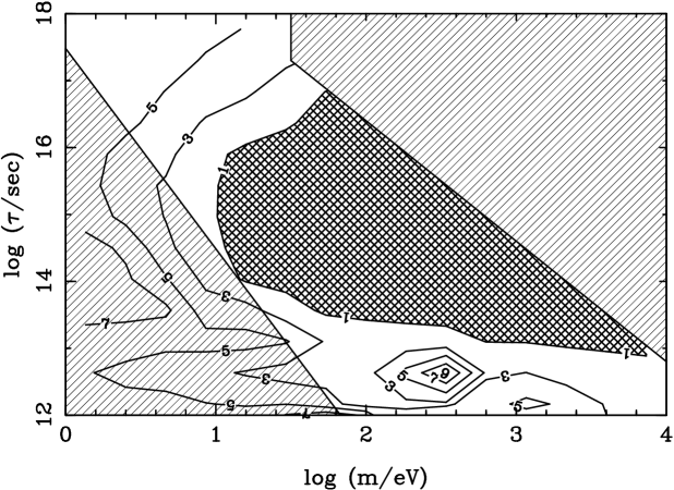
FIG. 3.: Contours of the peak $(l=200)$/plateau $(l=10)$ ratio for CMB spectra. sCDM predicts a ratio on the order of five; data certainly excludes values less than one. The upper right region of parameter space produces $\Omega>1$. The lower left hatched region is the bound on $\nu_{\tau}\rightarrow\nu_{\mu}+\phi$ from equation (1).

Model Dependence of the Constraint. The contours drawn in Figure 3 depend on the underlying cosmological model and associated set of parameters. How does the constraint hold up as these vary? Certainly, all of this work is predicated on the assumption that the primordial perturbations are adiabatic. This assumption at present seems well-motivated both theoretically and observationally[11]. Raising the Hubble constant to a value more consistent with present data lowers the peak. A higher $\Omega_{B}$ would help here, but our value of $0.08$ is about as high as possible, given constraints from Big Bang Nucleosynthesis[8]. We have also neglected reionization, but this too lowers the peak/plateau ratio even further. We have neglected tensor modes, but these too work in the wrong direction, falling off at $l\mathrel{\mathchoice{\lower 3.6pt\vbox{\halign{$\mathsurround=0pt\displaystyle\hfil#\hfil$\cr>\crcr\sim\crcr}}}{\lower 3.6pt\vbox{\halign{$\mathsurround=0pt\textstyle\hfil#\hfil$\cr>\crcr\sim\crcr}}}{\lower 3.6pt\vbox{\halign{$\mathsurround=0pt\scriptstyle\hfil#\hfil$\cr>\crcr\sim\crcr}}}{\lower 3.6pt\vbox{\halign{$\mathsurround=0pt\scriptscriptstyle\hfil#\hfil$\cr>\crcr\sim\crcr}}}}100$. Our model assumes that the decay products are sterile. However, our results also apply to photon-producing decays which occur after last scattering; such decays would also lead to a large ISW effect. But in the parameter range of interest, the photons produced in such decays would seriously distort the well-measured[12] thermal spectrum of the CMB or produce an (unobserved) diffuse photon background[13].

One parameter which could serve to produce a rise on small scales is the spectral index of the primordial perturbations, $n$, which we have set to one. Most inflationary models[14] predict values slightly smaller than one, which would again reduce even further the peak/plateau ratio. However, there are some models (e.g. hybrid inflation[15] and supernatural inflation [16]) which predict “blue” spectra ($n>1$). Even if we allow $n>1$, though, the vast majority of the excluded $m,\tau$ region in Figure 3 will remain excluded. To see why, consider Figure 4, which shows the spectrum for a set of excluded $m,\tau$ values. The spectrum can be modified to go through the data at $l\sim 200$ if $n=2.15$. Such an extreme value of $n$, however, is strongly disfavored at both higher and lower values of $l$.

FIG. 4.: Impact of varying the scalar spectral index. The solid line is the sCDM prediction. The dashed line is for a neutrino with $m=30$ eV and $\tau=10^{15}$ sec, while the dashed-dotted line is the same decaying neutrino model, but with a scalar spectral index $n=2.15$. This value was chosen to make the CMB exhibit a rise at $l\sim(100-200)$, as indicated by observations, shown here by the points. Note the poor fit of the tilted model at low and high values of $l$.

Finally, we have assumed a flat universe today ($\Omega=1$). An open universe, however, would only exacerbate this effect since the peak/plateau ratio is already relatively small in open models. This is true for two reasons. First, curvature-induced gravitational potential decays cause extra power at $l\sim 10$. Second, lowering $\Omega$ shifts the first acoustic peak to the right, lowering the anisotropy at $l\sim 200$. There is one interesting caveat to this argument. In an open universe, the ISW effect due to the decay products also shifts to larger $l$. For small enough lifetimes, the ISW peak could be shifted all the way to $l\sim 200$, mimicking the first acoustic peak in a flat universe! For example, a model with $m=30$ eV, $\tau=10^{13}$ sec and $\Omega=0.3$ gives an ISW peak near $l=200$ and a peak/plateau ratio $\sim 6$, in rough agreement with current observations.

Conclusions. An unstable neutrino with mass greater than $10$ eV and lifetime $10^{13}\mathrel{\mathchoice{\lower 3.6pt\vbox{\halign{$\mathsurround=0pt\displaystyle\hfil#\hfil$\cr<\crcr\sim\crcr}}}{\lower 3.6pt\vbox{\halign{$\mathsurround=0pt\textstyle\hfil#\hfil$\cr<\crcr\sim\crcr}}}{\lower 3.6pt\vbox{\halign{$\mathsurround=0pt\scriptstyle\hfil#\hfil$\cr<\crcr\sim\crcr}}}{\lower 3.6pt\vbox{\halign{$\mathsurround=0pt\scriptscriptstyle\hfil#\hfil$\cr<\crcr\sim\crcr}}}}\tau\mathrel{\mathchoice{\lower 3.6pt\vbox{\halign{$\mathsurround=0pt\displaystyle\hfil#\hfil$\cr<\crcr\sim\crcr}}}{\lower 3.6pt\vbox{\halign{$\mathsurround=0pt\textstyle\hfil#\hfil$\cr<\crcr\sim\crcr}}}{\lower 3.6pt\vbox{\halign{$\mathsurround=0pt\scriptstyle\hfil#\hfil$\cr<\crcr\sim\crcr}}}{\lower 3.6pt\vbox{\halign{$\mathsurround=0pt\scriptscriptstyle\hfil#\hfil$\cr<\crcr\sim\crcr}}}}10^{17}$ sec is ruled out by current CMB observations. These limits are quite robust to changes in the underlying cosmological model. Moreover, they apply generally to any massive particle species (e.g. a neutralino or gravitino) that contributes significantly to the energy density and decays in the post-decoupling time frame. They also rule out the possibility of a radiation dominated Universe, proposed in 1984 to solve the $\Omega$ problem [17]. Moving beyond current observations, precision measures of the CMB spectrum out to $l\sim 2000$, as expected from the MAP and PLANCK satellites[18], are capable of probing the mass/lifetime plane for all $m\mathrel{\mathchoice{\lower 3.6pt\vbox{\halign{$\mathsurround=0pt\displaystyle\hfil#\hfil$\cr>\crcr\sim\crcr}}}{\lower 3.6pt\vbox{\halign{$\mathsurround=0pt\textstyle\hfil#\hfil$\cr>\crcr\sim\crcr}}}{\lower 3.6pt\vbox{\halign{$\mathsurround=0pt\scriptstyle\hfil#\hfil$\cr>\crcr\sim\crcr}}}{\lower 3.6pt\vbox{\halign{$\mathsurround=0pt\scriptscriptstyle\hfil#\hfil$\cr>\crcr\sim\crcr}}}}1$ eV[19].

We thank U. Seljak and M. Zaldariagga for the use of CMBFAST[20], which we amended to include decaying neutrinos. This work is supported by the DOE and by NASA Grant NAG 5-7092.

REFERENCES

- [1] G. Gerstein & Ya. B. Zel’dovich, Zh. Eksp. Teor. Fiz. Pis’ma Red. 4, 174 (1966).
- [2] G. Marx & A. Szalay, in Neutrino ’72, eds. A. Frenkel & G. Marx, OMKDT-Technoinform, Budapest, (1972); R. Cowsik & J. McClelland, Phys. Rev. Lett.29, 669 (1972).
- [3] Particle Data Group, Phys. Rev. D54, 1 (1996).
- [4] R.N. Mohapatra & P.B. Pal, Massive Neutrinos in Physics and Astrophysics (Singapore: World Scientific, 1991)
- [5] M. Kawasaki, P. Kernan, H.-S. Kang., R.J. Scherrer, G. Steigman, & T.P. Walker, Nucl. Phys. B 419, 105 (1994).
- [6] See e.g. D. Scott and M. White, in the Proceedings of the CWRU CMB Workshop “2 years after COBE” eds. L. Krauss & P. Kernan (1994); or S. Hancock, G. Rocha, A. N. Lasenby & C.M. Gutierrez, MNRAS 294, L1 (1998).
- [7] C.L. Bennett et al., ApJ464, L1 (1996).
- [8] S. Burles & D. Tytler, astro-ph/803071 to appear in Proceedings of the Second Oak Ridge Symposium on Atomic & Nuclear Astrophysics, ed. A. Mezzacappa (1998).
- [9] W.Hu & N. Sugiyama, ApJ44, 489 (1995); Phys. Rev. D51, 259 (1995).
- [10] G. Steigman & M.S. Turner, Nucl. Phys. B 253, 375 (1985).
- [11] See e.g. S. Dodelson, E. Gates, and M.S. Turner, Science 274, 69 (1996).
- [12] D.J. Fixsen et al., ApJ486, 623 (1996); H.P. Nordberg & G.F. Smoot, astro-ph/9805123.
- [13] E. W. Kolb & M. S. Turner, The Early Universe (Addison-Wesley, Redwood City, CA, 1990), ch. 5.
- [14] See, e.g. D. Lyth, hep-ph/9609431; S. Dodelson, W. Kinney, & E. W. Kolb, Phys. Rev. D, 56, 3207 (1997).
- [15] A.Linde, Phys. Rev. D49, 748 (1994); J.Garcia-Bellido, A. Linde, & D.Wands, Phys. Rev. D, 54, 6040 (1996).
- [16] L. Randall, M. Soljacic, & A. Guth, Nucl. Phys. B472, 377 (1996).
- [17] M. S. Turner, G. Steigman, & L. Krauss, Phys. Rev. Lett.52, 2090 (1984); G. Gelmini, D. N. Schramm & Valle, Physics Letters 146, 311 (1984); D. Seckel, K. Olive, & E. Vishniac, ApJ292, 1 (1985).
- [18] Information about the satellites is available at http://map.gsfc.nasa.gov/ and http://astro.estec.esa.nl/SA-general/Projects/Planck.
- [19] Constraints on stable neutrinos have been explored in S. Dodelson, E.I. Gates, & A. Stebbins, ApJ467, 10 (1996); J.R. Bond, G. Efstathiou & M. Tegmark, MNRAS 291, L33 (1997). Unstable neutrinos are treated in M. White, G. Gelmini, & J. Silk, Phys. Rev. D51, 2669 (1995); S. Hannestad, astro-ph/9804075 (1998); J.A. Adams, S. Sarkar, & D.W. Sciama, astro-ph/9805108 (1998); S. A. Bonometto & E. Pierpaoli, astro-ph/9806035 (1998); E. Pierpaoli & S. A. Bonometto, astro-ph/9806037 (1998); R.E. Lopez, S. Dodelson, R.J. Scherrer, & M.S. Turner, in preparation (1998).
- [20] U. Seljak and M. Zaldarriaga, ApJ469, 437 (1996).