USITP/98-08
MPI-PhT/98-43
June 1998
 
Clumpy Neutralino Dark Matter

We investigate the possibility to detect neutralino dark matter in a scenario in which the galactic dark halo is clumpy. We find that under customary assumptions on various astrophysical parameters, the antiproton and continuum $\gamma$-ray signals from neutralino annihilation in the halo put the strongest limits on the clumpiness of a neutralino halo. We argue that indirect detection through neutrinos from the Earth and the Sun should not be much affected by clumpiness. We identify situations in parameter space where the $\gamma$-ray line, positron and diffuse neutrino signals from annihilations in the halo may provide interesting signals in upcoming detectors.

I Introduction

The mystery of the dark matter in the Universe remains unsolved. Among the more plausible candidates (not only needed to solve the dark matter problem) can be found the neutralino, the lightest supersymmetric particle in the Minimal Supersymmetric Standard Model (MSSM) (for a review, see [1]). Another candidate is for instance the axion which is still a viable option for a narrow range of axion masses [2]. Irrespective of the exact nature of the dark matter, there are reasons to believe that its distribution in the dark halos of galaxies need not be perfectly smooth [3, 4, 5]. For instance, early fluctuations in the dark matter may go non-linear long before photon decoupling, evading the argument of slow, linear growth after recombination. Also, if cosmic strings or other defects exist, they may seed the formation of density-enhanced dark matter clumps.

Since very little is known about the inherently non-linear problem of generating dark matter clumps, in this paper we will use a phenomenological approach where we simply assume the existence of clumps with a given density profile, making up a certain fraction of the total mass of the Milky Way halo. We investigate the effect of this clumpiness on the various proposed detection methods for neutralino dark matter. Detection rates depend crucially on the neutralino distribution in momentum and position space. Some detection rates, in particular those of antiprotons and photons generated by neutralino annihilations in the galactic halo, increase substantially compared to the case of a smooth dark matter distribution. For a given set of parameters of the supersymmetric models (such as mass and couplings of the neutralinos) we can then use present experimental limits on these fluxes to bound the degree of clumpiness allowed in that particular dark matter model. Alternatively, given a positive experimental signature, we can identify regions in the combined parameter space of halo dark matter distribution and supersymmetric models to identify candidates consistent with the data. This approach was used recently by three of us in connection with new data from the EGRET gamma ray detector [6]. Some of our results may be of interest also in the standard non-clumpy scenario, which is of course included in our treatment and is easily recovered by putting the fraction of the halo in the form of clumps equal to zero.

II Clumpiness in the Milky Way halo

Present observational data give very poor constraints on the distribution of dark matter in the galaxy. The dynamics of the outer satellites of the galaxy clearly indicates that luminous matter provides just a fraction of the total mass of the Milky Way and that the major contribution must come from a dark matter halo whose size is larger than the radius of the disk. Nevertheless it is not possible to extract from present kinematic information any accurate knowledge of the density profile of the dark matter halo. It is, however, natural to assume that galactic dark matter profiles obey a law of universality. Then, a possible approach is to infer the functional form of the Milky Way halo density profile from the results of $N$-body simulations of hierarchical clustering in cold dark matter cosmologies, fitting the normalization parameters to known dynamical constraints. This approach has been followed in Ref. [7]: among the general family of spherical density profiles,

$$\rho(\vec{x})=\rho_{0}\;\left(\frac{R_{0}}{|\vec{x}|}\right)^{\gamma}\,\left[\frac{1+(R_{0}/a)^{\alpha}}{1+(|\vec{x}|/a)^{\alpha}}\right]^{(\beta-\gamma)/\alpha},$$ (1)

it was considered the case of the Kravtsov et al. profile [8] which is mildly singular towards the galactic centre with $\gamma\sim 0.2$–$0.4$, of the Navarro et al. profile [9] which is more cuspy ($\gamma=1$), and, for comparison the modified isothermal distribution, $(\alpha,\beta,\gamma)=(2,2,0)$, extensively used in dark matter detection computations.

The dark matter density profile inferred in this way should be regarded as the function that describes the average distribution of dark matter in the galactic halo; the standard assumption which is generally made at this stage is that dark matter particles in the halo form a perfectly smooth ‘gas’. This approach is in some way arbitrary: although the dark matter particle distribution has to be regarded as smooth on intermediate length scales, probably around 0.01–1 kpc, there are reasons to question whether this is true on smaller scales. We here entertain the possibility that at least a fraction of the dark matter in the halo is clustered in substructures with high matter density, ‘clumps’ of dark matter. Several authors have introduced clumpiness as a generic feature of cold dark matter cosmologies. Silk and Stebbins [4] have considered clump formation in cosmic string, texture and inflationary models, giving also predictions for survival to tidal disruption (see also Ref. [3]). Kolb and Tkachev [5] have studied isothermal fluctuations giving very high-density dark matter clumps.

Simulations of structure formation in the early Universe do not yet have the dynamical range to give predictions for the size and density distribution of small mass clumps (we focus here mainly on clumps of less than around $10^{6}$ solar masses which avoid the problem of unacceptably heating the disk  [4]). The formation of clumps on all scales is however a generic feature of cold dark matter models which have power on all length scales. If self-similarity is a guide, galaxy halos may form hierarchically in a similar way to that of cluster halos (see e.g. Ref. [10]).

Rather than examining the different scenarios for clump formation, we take a more phenomenological approach and perform a detailed discussion on the implications of clumpiness on neutralino dark matter searches.

We thus simply postulate that a fraction $f$ of the total dark matter is concentrated in clumps, which are assumed to be spherical bodies of typical mass $M_{cl}$ and matter density profile $\rho_{cl}(\vec{r_{cl}})$. The total number of clumps inside the halo is given by:

$$N_{c}\sim\frac{f\,\cdot\,M_{h}}{M_{cl}}$$ (2)

where $M_{h}$ is the total mass of the halo. Two opposite scenarios seem to be plausible. There might be few heavy clumps, with masses up to maybe $M_{cl}\sim 10^{6}$–$10^{8}M_{\odot}$ (above which the local gravitational distortion effects would be too severe); such massive bodies could in principle be identified from the analysis of the rotation curves of the galaxy, they may however have escaped observation so far because their detection in this way may be difficult if the fraction of dark matter in clumps is small, say $f\sim 1\%$. A second possibility is that clumps are much lighter, with $M_{cl}$ less than $10^{4}$–$10^{6}M_{\odot}$, in which case larger fractions of the halo mass might be in clumps (in the extreme scenario all of it). In the many small clumps scenario, on which we mainly focus, we can define a probability density distribution of the clumps in the galaxy which in the limit of large $f$, to fulfill dynamical constraints, has to follow the mass distribution in the halo.

Consider a Cartesian coordinate system with origin in the galactic centre. Then the probability for a given clump being in the volume element $d^{\,3}x$ at position $\vec{x}$ is

$$p_{cl}(\vec{x})\,d^{\,3}x=\frac{1}{M_{h}}\;\rho(\vec{x})\,d^{\,3}x$$ (3)

which has the correct normalization $\int p_{cl}(\vec{x})d^{\,3}x=1$.

It is convenient to introduce the dimensionless parameter $\delta$

$$\delta=\frac{1}{\rho_{0}}\frac{\int d^{\,3}r_{cl}\,\left(\rho_{cl}(\vec{r_{cl}})\right)^{2}}{\int d^{\,3}r_{cl}\,\rho_{cl}(\vec{r_{cl}})}$$ (4)

which gives the effective contrast between the dark matter density in clumps and the local halo density $\rho_{0}$. For a dark matter density inside the clumps which is roughly constant, $\rho_{cl}$, it reduces to the form

$$\delta=\frac{\rho_{cl}}{\rho_{0}}\;.$$ (5)

We show in Section IV that in the many-clumps scenario it is just the product $f\delta$ which determines the increase of the signal compared to a smooth halo in most indirect detection methods. The product $f\delta$ is directly related to the ratio of the total dark mass in clumps to the volume of a typical clump.

III Supersymmetric models for dark matter

Although it is possible that the halo dark matter may be composed of particles not yet predicted by particle physics models, it is very attractive to assume that they are weakly interacting massive particles (WIMPs). Massive particles with weak interactions give a relic density which is of the right order of magnitude to explain the dark matter on all scales from dwarf galaxies and upwards. We will consider a specific class of such particles, supersymmetric particles, which is general enough to illustrate the effects of clumpiness. Our results should be of more general validity, however.

Parameter	$\mu$	$M_{2}$	$\tan\beta$	$m_{A}$	$m_{0}$	$A_{b}/m_{0}$	$A_{t}/m_{0}$
Unit	GeV	GeV	1	GeV	GeV	1	1
Min	-50000	-50000	1.0	0	100	-3	-3
Max	50000	50000	60.0	10000	30000	3	3

TABLE I.: The ranges of parameter values used in our scans of the MSSM parameter space. Note that several special scans aimed at interesting regions of the parameter space have been performed. In total we have generated about 85000 models that are not excluded by accelerator searches.

We work in the Minimal Supersymmetric Standard Model (MSSM) as defined in Refs. [11, 1]. For details on our notation, see Ref. [12]. The lightest stable supersymmetric particle is in most models the neutralino, which is a superposition of the superpartners of the gauge and Higgs fields,

$$\tilde{\chi}^{0}_{1}=N_{11}\tilde{B}+N_{12}\tilde{W}^{3}+N_{13}\tilde{H}^{0}_{1}+N_{14}\tilde{H}^{0}_{2}.$$ (6)

It is convenient to define the gaugino fraction of the lightest neutralino,

$$Z_{g}=|N_{11}|^{2}+|N_{12}|^{2}$$ (7)

For the masses of the neutralinos and charginos we use the one-loop corrections as given in [13].

The MSSM has many free parameters, but with some simplifying assumptions, we are left with 7 parameters, which we vary between generous bounds. The ranges for the parameters are shown in Table I. For the detection rates of neutralino dark matter we have used the rates as calculated in Refs. [6, 7, 14, 15, 16, 17].

We will throughout this paper assume that the neutralinos make up most of the dark matter in our galaxy. We only consider therefore MSSM models which are cosmologically interesting, i.e. where the neutralinos can make up a major fraction of the dark matter in the Universe without overclosing it. We will choose this range to be $0.025<\Omega_{\chi}h^{2}<0.5$. For the relic density calculations we have used the detailed calculations performed in Ref. [12].

IV Detection methods constraining clumpiness

Some observational consequences of a clumpy dark matter halo have been pointed out previously, such as the obvious gain in gamma ray signal from annihilation in the halo since the flux from a particular volume element is proportional to the square of the dark matter density there [4, 5, 18, 19, 20, 21]. Also, in Ref. [22] it was noted that the antiproton flux could be enhanced, although the treatment was sketchy and not entirely correct concerning the way the rescaling was done. In Ref. [23], it was investigated whether encounters with dark matter clumps on geophysical time scales could have left imprints in ancient mica.

As we show in this section, indirect detection through cosmic antiprotons and gamma rays set the most stringent limits on clumpy neutralino dark matter, therefore we investigate these cases first.

A Gamma-rays

Since gamma rays produced in neutralino annihilations in the halo travel in straight paths essentially without any absorption, and since the annihilation rate and hence the flux would be enhanced by clumps along a particular line-of-sight, the effects of clumpiness are easy to understand.

Neutralino annihilation in the galactic halo may produce both a $\gamma$-ray flux with a continuum energy spectrum and monochromatic $\gamma$-ray lines.

The continuum contribution (see Ref. [1] and references therein) is mainly due to the decay of $\pi^{0}$ mesons produced in jets from neutralino annihilations. To model the fragmentation process and extract information on the number and energy spectrum of the $\gamma$s produced we have used the Lund Monte Carlo Pythia 6.115 [24]. We have performed the simulation for 18 neutralino masses between 10 and 5000 GeV and for the $c\bar{c}$, $b\bar{b}$, $t\bar{t}$, $W^{+}W^{-}$, $Z^{0}Z^{0}$ and $gg$ annihilation states. For each final state and for each neutralino mass we have simulated $2.5\times 10^{5}$ events which are tabulated logarithmically in energy. For any given MSSM model, we then sum over the annihilation channels and interpolate in these tables. For the annihilation channels not included in the simulations, like the ones with one gauge and one Higgs boson as well as those with two Higgs bosons the flux is calculated in terms of the flux from the simulated channels. We include all two-body final states at the tree level (except light quarks and leptons) and the one-loop processes $Z\gamma$ and $gg$. For final states with Higgs bosons, we let the Higgs bosons decay in flight by summing the contributions to the gamma flux from the Higgs decay products in the Higgs rest system and then boost the spectrum averaging over decay angles. Given the annihilation branching ratios we then get the spectrum for any given MSSM model. The continuum signal lacks distinctive features and it might be difficult to discriminate from other possible sources. It will however be a powerful tool to put constraints on the clumpiness parameters.

A much better signature than the continuum contribution is given by monochromatic $\gamma$-ray lines which arise from the loop-induced S-wave neutralino annihilations into the $2\gamma$ and $Z\gamma$ final states and which have no conceivable background from known astrophysical sources. The amplitude of these two processes in the MSSM was computed only recently at full one loop level [25, 26]. Large deviations from previous partial results (see Ref. [1] and references therein) were found, in particular it was pointed out that a pure heavy Higgsino has a remarkably high annihilation branching ratio both into $2\gamma$ and $Z\gamma$, adding at least a factor of 10 to previous estimates of the $2\gamma$ line. A detailed phenomenological study is given in Ref. [7] where a smooth halo scenario was considered and it was shown that the monochromatic lines could be detected by the new generation of space- and ground-based $\gamma$-ray experiments, provided that a sensible enhancement of the dark matter density is present towards the galactic centre. We examine here the perspectives of detecting the continuum and the line signals in a given clumpy scenario.

Consider a detector with an angular acceptance $\Delta\Omega$ pointing in a direction of galactic longitude and latitude $(\ell,b)$. The gamma ray flux from neutralino annihilations at a given energy $E$ is given by

$$\Phi_{\gamma}(E,\,\Delta\Omega,\,\ell,\,b)\simeq 1.87\cdot 10^{-8}\,\frac{d{\cal S}}{dE}\,\langle\,J\left(\ell,\,b\right)\,\rangle\,(\Delta\Omega)\;\;\rm{cm}^{-2}\;\rm{s}^{-1}\;\rm{sr}^{-1}\;.$$ (8)

In this formula we have defined a factor $d{\cal S}/dE$ which depends on the nature of relic WIMPs. For the continuum $\gamma$-ray signal, the $2\gamma$ line and the $Z\gamma$ line signal, respectively, it is given by:

$$\left(\frac{d{\cal S}}{dE}\right)_{{\rm cont.}~{}\gamma} \simeq \left(\frac{10\,\rm{GeV}}{M_{\chi}}\right)^{2}\cdot\sum_{F}\left(\frac{v\sigma_{F}}{10^{-26}\ {\rm cm}^{3}\;{\rm s}^{-1}}\right)\,\frac{dN_{\gamma}^{\,F}}{dE}$$ (9)

$$\left(\frac{d{\cal S}}{dE}\right)_{2\gamma} \simeq \left(\frac{10\,\rm{GeV}}{M_{\chi}}\right)^{2}\,\left(\frac{2\;v\sigma_{2\gamma}}{10^{-26}\ {\rm cm}^{3}\;{\rm s}^{-1}}\right)\,\delta\left(E-M_{\chi}\right)$$ (10)

$$\left(\frac{d{\cal S}}{dE}\right)_{Z\gamma} \simeq \left(\frac{10\,\rm{GeV}}{M_{\chi}}\right)^{2}\,\left(\frac{v\sigma_{Z\gamma}}{10^{-26}\ {\rm cm}^{3}\;{\rm s}^{-1}}\right)\,\delta\left(E-M_{\chi}\,\left(1-\frac{{M_{Z}}^{2}}{4\,{M_{\chi}}^{2}}\right)\right).$$ (11)

Here $M_{\chi}$ is the neutralino mass, $F$ are the allowed final states which contribute to the continuum signal as specified above. For each of these, $v\sigma_{F}$ is the annihilation rate and $dN_{\gamma}^{\,F}/dE$ is the differential energy distribution of produced photons. The product of relative velocity and cross section $v\sigma_{2\gamma}$ is the annihilation rate into the $2\gamma$ final state (as given in Ref. [25]). Similarly, $v\sigma_{Z\gamma}$ is the rate into the $Z\gamma$ final state (as given in Ref. [26]). In Eq. (8) the dependence of the flux on the dark matter distribution, the direction of observation $(\ell,b)$ and the angular acceptance of the detector $\Delta\Omega$ is contained in the factor $\langle\,J\left(\ell,\,b\right)\,\rangle\,(\Delta\Omega)$. If we assume a spherical dark matter halo in the form of a perfectly smooth distribution of neutralinos, it is equal to

$$\langle\,J\left(\psi\right)\,\rangle\,(\Delta\Omega)=\frac{1}{8.5\,\rm{kpc}}\,\frac{1}{\Delta\Omega}\;\int_{\Delta\Omega}\,d\Omega^{\prime}\;\int_{line\;of\;sight}\,dL\;\left(\frac{\rho(L,\,\psi^{\prime})}{0.3\,{\rm GeV}/{\rm cm}^{3}}\right)^{2}\;.$$ (12)

Here $L$ is the distance from the detector along the line of sight, $\psi$ is the angle between the direction of observation and that of the galactic center, related to $(\ell,\,b)$ by $\cos\psi=\cos\ell\,\cos b$. The integration over $d\Omega^{\prime}$ is performed over the solid angle $\Delta\Omega$ centered on $\psi$.

We shall now examine the consequences of introducing clumps in the halo. The continuum $\gamma$-ray signal in the few clumps scenario has as mentioned been examined in some detail in the literature. Following the approach of Refs. [18, 19] and estimating the most probable distance for the nearest clump, we find in terms of the quantities introduced above that $\langle\,J\,\rangle$ in the direction of the nearest clump is of the order

$$\langle\,J\left(\psi_{cl}\right)\,\rangle\,(\Delta\Omega)\mathrel{\hbox to0.0pt{\lower 4.0pt\hbox{\hskip 1.0pt$\sim$}\hss}\raise 1.0pt\hbox{$>$}}\left(\frac{4\,\pi}{3}\right)^{2/3}\,\frac{\delta}{8.5\,\rm{kpc}}\,\frac{1}{\Delta\Omega}\left(f^{2}\,\frac{M_{cl}}{\rho_{0}}\right)^{1/3}\;,$$ (13)

where the density profile inside the clump was considered roughly constant and the angular acceptance of the detector $\Delta\Omega$ was supposed to be greater or equal to the field of view of the clump $\Delta\Omega_{cl}\sim(f/\delta)^{2/3}$. We consider as an example the same choice of parameters as in Ref. [19]: $f\sim 0.01$, $M_{cl}\sim 10^{8}M_{\odot}$, $\delta\sim 10^{3}$. In this case we find $\Delta\Omega_{cl}\sim 4\cdot 10^{-4}$ sr, and taking $\Delta\Omega=10^{-3}$ sr, we obtain $\langle\,J\left(\psi_{cl}\right)\,\rangle\,\sim 3\cdot 10^{4}$ which we can compare with the analogous quantity in a smooth halo scenario. In Fig. 7 of Ref. [7] the values of $\langle\,J\,\rangle\,(\Delta\Omega=10^{-3}\rm{~{}sr})$ for a detector with $\Delta\Omega=10^{-3}\rm{~{}sr}$ pointing towards the galactic centre are displayed (see also our Fig. 1); the value of $\langle\,J\left(\psi_{cl}\right)\,\rangle$ is about one half of the value for the most singular Navarro et al. profile, which gives detectable $\gamma$-ray lines for a relevant portion of MSSM models.

The clump in our example might therefore be a very bright dark matter source, and a signal from neutralino annihilation into monochromatic photons in its direction could potentially be detected with an Air Cherenkov Telescope (ACT). In practice, the probability is small of detecting such a signal randomly pointing an instrument with a small angular acceptance. It might be of some help to combine ground- and satellite-based observations. A satellite detector, which has a wide field of view but also a much smaller effective area with respect to an ACT, may search in the continuum $\gamma$-ray spectrum for brighter spots in the sky which have no luminous counterpart. Such signals might then be identified as clumps of dark matter if one would detect with an ACT the $\gamma$-ray lines from neutralino annihilations. For such a method to be practical, higher overdensities $\delta$ may be needed. It should also be kept in mind that Eq. (13) gives just a qualitative feature of the possible result; the possibility for the nearest clump of being much further away or a more realistic density profile may change that result by orders of magnitude.

Much firmer predictions may be formulated in the many small clumps scenario; in this case we assume that most of the clumps cannot be resolved even by a detector with a rather small angular acceptance, say about $\Delta\Omega\sim 10^{-3}$ sr. There might still be some clumps which are resolvable just because they happen to be nearby and these should be treated as in the previous case.

From Eq. (3), the probability for a clump of being at a line of sight distance $(L,\,L+dL)$, a viewing angle defined by $(\cos\psi,\,\cos\psi+d\cos\psi)$ and at some azimuthal angle with respect to the direction of the galactic center $(\phi,\,\phi+d\phi)$ is given by

$$p_{cl}(L,\psi)\;dL\,d\cos\psi\,d\phi=\frac{1}{M_{h}}\;\rho(L,\psi)\,L^{2}\;dL\,d\cos\psi\,d\phi\;.$$ (14)

Assuming that the clumps can be regarded as point-like sources, we can derive the analogue of Eq. (12) (as in the latter we factorize out 1/4$\pi$):

$$\langle\,J(\psi)\,\rangle\,(\Delta\Omega) = \frac{1}{8.5\,\rm{kpc}}\,\frac{N_{cl}}{\Delta\Omega}\;\int_{\Delta\Omega}\,d\Omega^{\prime}\;\int_{line\;of\;sight}\,dL\;p_{cl}(L,\psi^{\prime})\cdot$$ (16)

$$\cdot\frac{1}{L^{2}}\,\int d^{\,3}r_{cl}\,\left(\frac{\rho_{cl}(\vec{r_{cl}})}{0.3\,{\rm GeV}/{\rm cm}^{3}}\right)^{2}.$$

Taking Eqs. (2) and (14) into account, this can be rewritten as

$$\langle\,J(\psi)\,\rangle\,(\Delta\Omega) \sim \frac{1}{8.5\,\rm{kpc}}\,\frac{f\delta}{\Delta\Omega}\left(\frac{\rho_{0}}{0.3\,{\rm GeV}/{\rm cm}^{3}}\right)\cdot$$ (18)

$$\cdot\int_{\Delta\Omega}\,d\Omega^{\prime}\;\int_{line\;of\;sight}\,dL\;\left(\frac{\rho(L,\psi^{\prime})}{0.3\,{\rm GeV}/{\rm cm}^{3}}\right)\;.$$

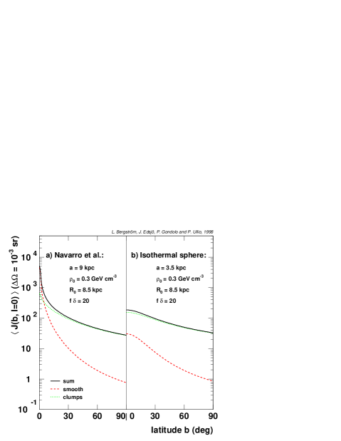
FIG. 1.: The value of $\langle\,J(\psi)\,)\rangle\,(\Delta\Omega)$ for two different halo profiles. The contribution from the smooth and clumpy component are also given.

Comparing Eq. (18) with Eq. (12), we realize that in a scenario with many small clumps the angular dependence of the signal is different from the one in the smooth halo scenario. This is illustrated in Fig. 1 for two different halo models, picking as an example $f\delta=20$: a Navarro et al.  profile (Eq. (1) with $(\alpha,\beta,\gamma)=(1,2,1)$ and, in our example, $\rho_{0}=0.3$ GeV/cm³, $a=9$ kpc) and a modified isothermal sphere (Eq. (1) with $(\alpha,\beta,\gamma)=(2,2,0)$, $\rho_{0}=0.3$ GeV/cm³, $a=3.5$ kpc). The parameter $f\delta$ mainly determines the relative importance of the smooth and clumpy components. An interesting feature, shown in the Figure for the Navarro et al. profile, is a possible break in the angular spectrum. This could be a possible signature to discriminate the signal from neutralino annihilations into continuum $\gamma$-rays from the galactic $\gamma$-ray background, and may be indeed suggested by a recent analysis of EGRET data [6].

We are now ready to give predictions for the $\gamma$-ray flux from neutralino annihilations. To minimize the impact of the halo model and of experimental uncertainties, we concentrate on the flux at high latitudes, $b>60^{\circ}$ and $0^{\circ}<\ell<360^{\circ}$ ($\Delta\Omega=0.84$ sr), rather than considering the flux towards the galactic centre which as shown in Fig. 1 is maximal. The modified isothermal profile of Fig. 1 gives

$$\langle\,J(90^{\circ})\,\rangle^{smooth}\,(0.84sr)+\langle\,J(90^{\circ})\,\rangle^{clumps}\,(0.84sr)\simeq 0.93\cdot(1+1.8\cdot f\delta)\;.$$ (19)

For simplicity we have made the reasonable assumption that $f$ is small. If that is not true we have to replace $1$ by $(1-f)^{2}$ in the above equation (as well as Eq. (25) below). The analogous estimates with any of the halo models considered in Ref. [7] are within a factor of 2 of the value given in Eq. (19). There is therefore a very weak halo model dependence in these results. In Fig. 2 (a) we plot the integrated $\gamma$-ray flux above the energy threshold $E_{th}=1$ GeV for our set of MSSM models in the smooth halo scenario. Also shown in the figure is the corresponding $\gamma$-ray flux measured by the Energetic Gamma Ray Experiment Telescope (EGRET) as inferred from the analysis in Ref. [27]:

$$\Phi_{\gamma}(E>1~{}\rm{GeV})=(1.0\pm 0.2)\times 10^{-6}~{}\mbox{cm${}^{-2}$ s${}^{-1}$ sr${}^{-1}$}\;.$$ (20)

We can compare with this value to obtain a constraint on the allowed values of the parameter $f\delta$. It is however useful to analyse this together with the analogous constraint we can derive in the scenario of many small clumps from neutralino annihilations into cosmic ray antiprotons.

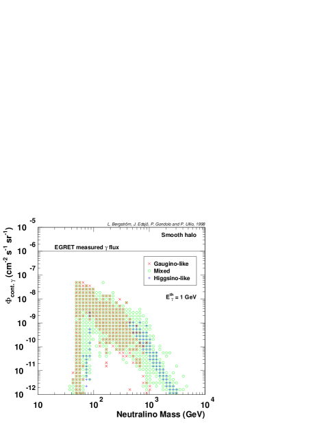
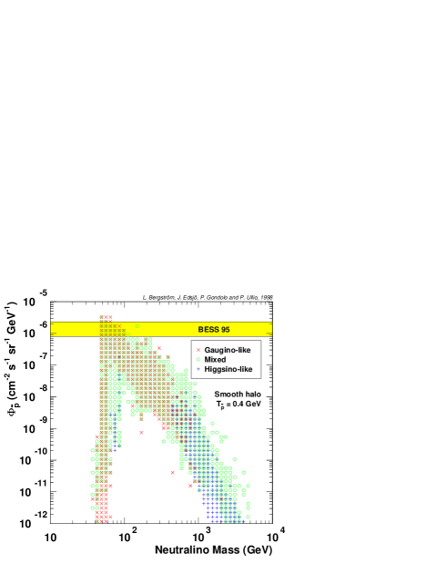
FIG. 2.: The signal of (a) continuum gamma and (b) antiprotons versus the neutralino mass. Only models with $0.025<\Omega_{\chi}h^{2}<0.5$ have been included in this and the following figures.

B Antiprotons

Neutralino annihilations of relic neutralinos in the galaxy may produce cosmic ray antiprotons ([1] and references therein, [22, 28]) mainly from jets, in a process which is analogous to the case of continuum $\gamma$-rays. To model the fragmentation process and extract information on the number and energy spectrum of the antiprotons produced we have again used the Lund Monte Carlo Pythia 6.115 and applied the same tabulation technique as for the production of photons. Including the same set of final states and treating the Higgs bosons in the same way, for any given MSSM model we can then obtain the energy spectrum of antiproton dark matter sources.

If we assume a smooth distribution of WIMPs in the galaxy, the production rate of antiprotons in the volume element $d^{\,3}x$ at the galactic position $\vec{x}$ is given by

$$\frac{d{\cal R}_{sm}(\vec{x})}{dT}\,d^{\,3}x=\left(\frac{\rho(\vec{x})}{M_{\chi}}\right)^{2}\cdot\sum_{F}v\sigma_{F}\,\frac{dN_{\bar{p}}^{\,F}}{dT}\;d^{\,3}x$$ (21)

where $T$ is the kinetic energy of the antiprotons. We will not discuss here the few-clumps scenario as those predictions are extremely sensitive to the parameters which define the model. We focus instead on the many small clumps scenario, treating again single clumps as point-like sources. In this case we find:

$$\frac{d{\cal R}_{cl}(\vec{x})}{dT}\,d^{\,3}x = N_{cl}\,p_{cl}(\vec{x})\;\int d^{\,3}r_{cl}\,\rho_{cl}^{2}(\vec{r_{cl}})\;\cdot\sum_{F}v\sigma_{F}\,\frac{dN_{\bar{p}}^{\,F}}{dT}\;d^{\,3}x$$ (22)

$$= f\,\delta\;\frac{\rho_{0}\;\rho(\vec{x})}{{M_{\chi}}^{2}}\cdot\sum_{F}v\sigma_{F}\,\frac{dN_{\bar{p}}^{\,F}}{dT}\;d^{\,3}x\;.$$ (23)

It is not straightforward to simulate the propagation of charged particles in the galaxy. Different models have been proposed, and no consensus has been established yet. We present results in the limit in which the propagation is modeled by pure diffusion, using the analytic solution derived in Ref. [28] to which we refer for further details.

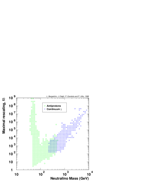
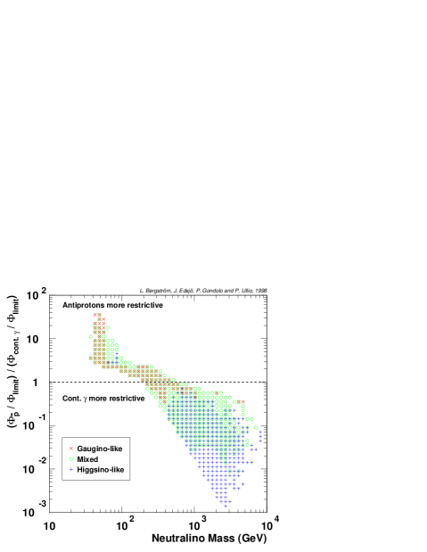
FIG. 3.: The maximal rescaling allowed by the present limits on the antiproton flux and the continuum gamma ray flux.

The BESS collaboration [30] has in a recent measurement of cosmic ray antiprotons found that the spectrum for the antiproton flux versus the kinetic energy $T$ is consistent with being flat for $T$ in the range between 180 MeV and 1.4 GeV. We consider the value of the measured flux at some low value of the kinetic energy, where the ‘trivial’ antiproton flux generated by cosmic-ray reactions in the interstellar medium is believed to be less dominant. At $T=400$ MeV the result found by BESS is

$$\Phi_{\bar{p}}(T=400~{}\rm{MeV})=1.4^{+0.9}_{-0.6}\times 10^{-6}~{}\bar{p}~{}\mbox{cm${}^{-2}$ s${}^{-1}$ sr${}^{-1}$ GeV${}^{-1}$}\;.$$ (24)

In Fig. 2 (b) we compare this value with the predictions for antiprotons from neutralino annihilations in a smooth halo scenario (i.e. the source given as in Eq. (21)) at the same energy, using for the diffusion model the same set of parameters as in Ref. [28], considering appropriate values of the solar modulation parameters and picking as halo profile the modified isothermal distribution. It is indeed tempting to conclude that some of our models are already excluded by the BESS measurement. However, one has to keep in mind the big uncertainties involved, mainly in the antiproton propagation; for instance it is not clear how large a fraction of antiprotons generated in the halo can penetrate the wind of cosmic rays leaving the disk [29]. We introduce in the flux predictions a rescaling factor $k$ which contains the uncertainties deriving from the choice of the parameters which define the propagation model considered and from possible deviations from this simple approach.

We consider now the many small clumps scenario. The production rate of antiprotons in this case is given by Eq. (21); the strength of the signal compared to the smooth case is again mainly determined by the product $f\delta$. At $T=400$ MeV and for the same halo profile considered above, we find:

$$\Phi_{\bar{p}}=k(1+0.75\cdot f\delta)\cdot\Phi_{\bar{p}}^{smooth}.$$ (25)

We have checked that the coefficient $0.75$ depends very weakly on the halo profile considered and on $T$. A conservative limit on the clumpiness parameter $f\delta$ can be obtained choosing the uncertainty factor $k$ as

$$k\in[0.2,5]\;.$$ (26)

We consider a value of $f\delta$ excluded if the whole range of possible antiproton fluxes given by Eqs. (25) and (26) exceeds the measured value, Eq. (24).

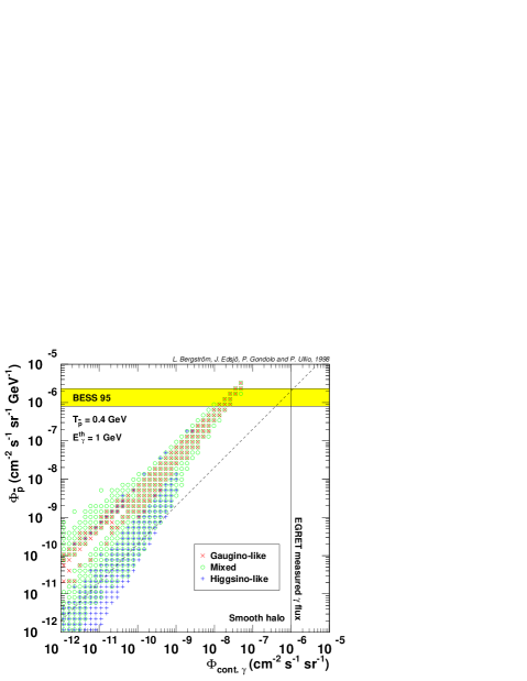
FIG. 4.: The antiproton flux versus the continuum $\gamma$ flux for a smooth halo.

C Determining the clumpiness factor $f\delta$

We have shown that in the many small clumps scenario the signals from dark matter annihilations into $\gamma$-rays and antiprotons depend critically on the clumpiness parameter $f\delta$. Focusing on the MSSM, we use the rescalings derived in Eqs. (19) and (25) to determine for each supersymmetric model the maximal value of $f\delta$ for which the experimental constraints on the fluxes of continuum photons and antiprotons are not violated. This is shown in Fig. 3 (a), where the maximal rescaling is given versus the neutralino mass, and where we use different symbols to indicate which of the two bounds is more restrictive. As can be seen, the antiproton flux puts the highest constraints on the clumpiness at low masses, whereas the continuum gammas put better constraints at higher masses. We see that the present experimental limits constrain $f\delta\mathrel{\hbox to0.0pt{\lower 4.0pt\hbox{\hskip 1.0pt$\sim$}\hss}\raise 1.0pt\hbox{$<$}}10^{9}$ for all masses.

As shown in Fig. 4, the two signals are strongly correlated since they are both produced from jets. In this sense the information we get from the two experimental limits is not entirely complementary. At higher masses, both fluxes go down since they are both proportional to $1/M_{\chi}^{2}$, but the correlation also decreases since the antiproton fluxes are only given in a small energy interval while the gamma ray fluxes are integrated above a threshold. Hence the antiproton flux in a given low energy interval decreases more than the gamma ray flux as we go to higher neutralino masses. In Fig. 3 (b) we analyse how restrictive one detection method is compared to the other.

Having derived for each of the MSSM models in our sample the maximal allowed value for the clumpiness parameter $f\delta$, in the next section we analyse the consequences of this result for other indirect detection methods of neutralino dark matter.

V Other detection methods

In this section we consider the many small clumps scenario with the highest possible value of $f\delta$ as given in the previous section and investigate what effect that has on other dark matter searches. We fix again as smooth halo distribution to compare with the modified isothermal distribution, Eq. (1) with $(\alpha,\beta,\gamma)=(2,2,0)$, $\rho_{0}=0.3$ GeV cm^-3, $a=3.5$ kpc and $R_{0}=8.5$ kpc.

A Monochromatic $\gamma$-ray lines

As we have seen, the same scaling applies to the continuum and the line $\gamma$-ray signals, it is therefore straightforward to derive the maximal fluxes of monochromatic photons from neutralino annihilations.

We perform this analysis in light of the potential of the next generation of satellite-based $\gamma$-ray detectors, and in particular of the proposed Gamma-ray Large Area Space Telescope (GLAST) [31]. To prevent uncertainties due to the choice of the dark matter halo profile to play any role in the following discussion, we fix again as field of view a 0.84 sr cone in the direction $b=90^{\circ}$. In the actual experiment the detector will collect data with a $4\pi$ sr angular acceptance; as for most halo profiles the ratio signal to squared root of the background is greatly enhanced towards the galactic centre, the predictions we show are an underestimate of the possible results.

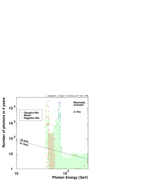
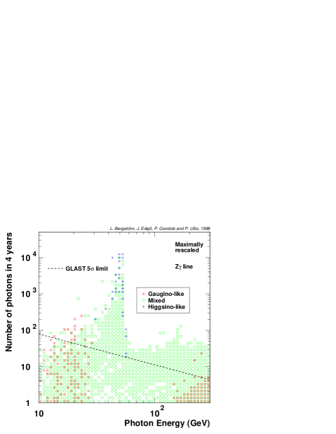
FIG. 5.: The number of expected photons in 0.84 sr towards $b=90^{\circ}$ collected in 4 years from (a) the $2\gamma$ and (b) the $Z\gamma$ final states. The expected $5\sigma$ limit from the GLAST detector is also shown.

Taking into account the screening of the earth, the useful geometrical acceptance of GLAST towards a fixed point of the sky in a 0.84 sr cone is 0.21 m² sr [32]; the energy resolution is assumed to be 1.5%. We display in Fig. 5 the number of expected $\gamma$s in 4 years of exposure time when the fluxes have been maximally rescaled according to Fig. 3. Also shown is the curve giving the minimum number of events needed to observe an effect at the $5\sigma$ level, where, in lack of data, we have assumed above 1 GeV a 2.7 power law falloff for the diffuse $\gamma$-ray background and inferred its normalization from Ref. [27]. As can be seen, a fair fraction of our set of supersymmetric models can be probed under these circumstances. Remember that the number of photons given in Fig. 5 is towards $b=90^{\circ}$ and, depending on halo profile, we expect more events towards the galactic centre, with a larger portion of the MSSM parameter space which might be probed.

B Diffuse neutrinos

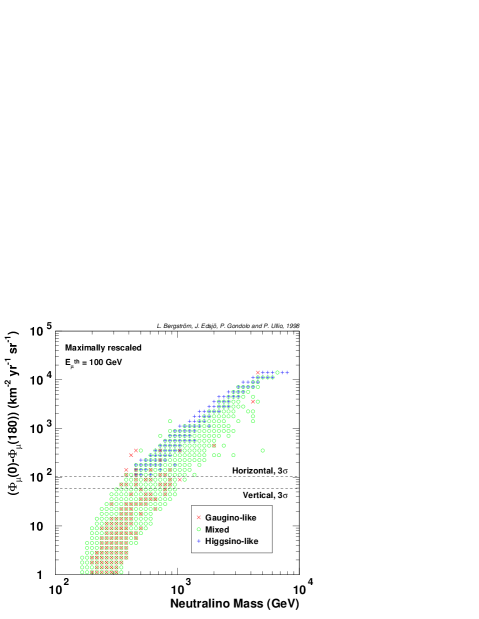
FIG. 6.: The difference of the diffuse neutrino flux towards the galactic centre to that to the antigalactic centre. The fluxes are averaged over 2.5 sr which maximizes signal to noise and they are rescaled maximally as allowed by the antiproton and continuum $\gamma$ fluxes. The limits are for a neutrino telescope with an exposure of 10 km² yr.

A possibility to get a detectable neutrino flux from WIMP annihilations which has rarely been considered in the literature is neutrinos from annihilation in the galactic halo. Of particular importance is $\chi\chi\to W^{+}W^{-}$, since the $W$ bosons decay in 10 % of the cases directly to a muon plus a muon neutrino with a hard neutrino spectrum, which may facilitate detection in neutrino telescopes.

This flux would scale in exactly the same way as the gamma flux in the presence of clumps and with future $\cal O$ (km³) neutrino-telescopes, the diffuse neutrinos might prove more constraining than antiprotons and continuum $\gamma$s at high masses (several hundred GeV – TeV region) where the rescaling can be high ($f\delta>10^{3}$).

The flux has been calculated in essentially the same way as for neutralino annihilation in the Sun/Earth [15] with the help of the Lund Monte Carlo Pythia 6.115. The only difference is that some annihilation products will decay and produce neutrinos in the halo, whereas they are stopped before they decay in the Sun/Earth.

The neutrino-induced muon flux from neutralino annihilations in a smooth halo is about $10^{-8}$–1 km^-2 yr^-1 sr^-1 above 100 GeV. Compare this with the atmospheric background of about 9500 km^-2 yr^-1 sr^-1 vertically and 30000 km^-2 yr^-1 sr^-1 horizontally [33] for this threshold. To be able to distinguish the signal from the background we have to rescale the fluxes by the allowed clumpiness factor derived in the previous section and we also have to make use of the fact that the signal is enhanced towards the centre of the galaxy.

The best prospects are probably given by large-area neutrino telescopes with relatively high detection thresholds. We can imagine measuring the flux in a solid angle $\Delta\Omega$ towards the galactic centre and compare with the flux in the same solid angle in the opposite direction. The limit we can put on the flux is at the $3\sigma$-level approximately given by

$$\left[\Phi_{\mu}(0^{\circ})-\Phi_{\mu}(180^{\circ})\right]_{\rm limit}\simeq 3\sqrt{\frac{\Phi_{bkg}}{{\cal E}\Delta\Omega}}.$$ (27)

where $\cal E$ is the exposure. For the modified isothermal sphere, it turns out the best limits are obtained with $\Delta\Omega=2.5$ sr, for which we obtain $\langle J(0^{\circ})\rangle(\Delta\Omega)=4.16$ and $\langle J(180^{\circ})\rangle(\Delta\Omega)=1.09$. In Fig. 6 we show the difference of the diffuse neutrino flux towards the galactic centre to that in the opposite direction for a muon energy threshold of 100 GeV. Also shown are the limits that can be reached with an exposure of 10 km² yr. For different exposures, the limits change as the square root of the exposure. If we increase the threshold from 100 GeV, we can gain a small factor in sensitivity at higher masses, but lose at intermediate masses.

An ideal neutrino detector for this signal would view the galactic center through the center of the Earth (i.e. it should be at 29 degrees latitude), since then the atmospheric background is minimal. The strength of the signal of course depends on the halo profile, but it is more likely that the halo profile is steeper towards the galactic centre than the isothermal sphere and hence the signal is even bigger then envisioned here. We might have to worry about other sources of high-energy neutrinos at the galactic centre (like neutrinos from the black hole believed to exist in the centre). These other sources can probably be removed by not looking at the very centre of the galaxy.

C Positrons

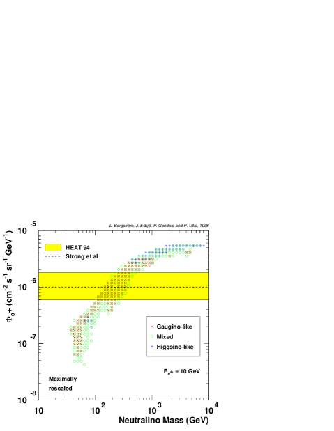
FIG. 7.: The positron fluxes rescaled maximally as allowed by the antiproton and continuum $\gamma$ fluxes. The 1994 HEAT measurement at 10 GeV [35] is shown together with the Strong et al. [38] prediction for the background at this energy.

From neutralino annihilation in the halo we would also get a flux of positrons which might be detected by satellite [34] or high-flying balloon experiments [35]. The propagation of positrons is a more difficult issue than for antiprotons since positrons are so easily deflected and destroyed. We have calculated the positron fluxes using Pythia 6.115 [24] and have used the propagation model in Ref. [36] with an energy dependent escape time (a more detailed investigation is in preparation [37]). In Fig. 7 we show the positron fluxes versus the neutralino mass when they have been rescaled with the maximal $f\delta$ allowed by the antiproton and the continuum gamma fluxes. We compare with the measurement by the HEAT experiment [35] at 10 GeV. Also shown is the prediction of the background at this energy as given in Ref. [38]. It would seem that the positrons put more stringent bounds on $f\delta$ than the antiprotons and continuum $\gamma$s at higher masses. The positron fluxes are however even more uncertain than the antiproton fluxes and can easily be wrong by a factor of 10. Hence we can’t use the positrons to constrain $f\delta$ further, but we see that we might be able to get measurable fluxes.

D Direct detection

For the direct rates, we have used the procedures in Ref. [14]. Since these rates only depend on the local halo density at present, they will as expected not put any severe constraints on the clumpiness of the halo as a whole. They will of course be much enhanced if we happen to be inside a clump at present. As with the neutrinos from neutralino annihilation in the Sun/Earth we can however have correlations between these signals and the signals giving high $\bar{p}$ or $\gamma$ fluxes. These correlations are not very strong, however.

E Neutralino annihilation in the Earth/Sun

Neutrinos are produced in the annihilations through the decays of quarks, leptons and gauge bosons produced in the primary annihilation process. During the several billion years the Earth and Sun have existed, there may have been a substantial accumulation of neutralinos due to capture, i.e. scattering and subsequent gravitational trapping.

The fluxes of neutrino-induced muons from neutralino annihilation in the Earth/Sun are mostly determined by the capture rates, which in turn depend on the local halo density. They are thus insensitive to different halo profiles; if the halo is clumped, there can however be fluctuations in the capture rates by time, but on the average we will capture the same amount of neutralinos as without clumps. The amount of these fluctuations in capture rate and consequently in annihilation rate depends on the time between encounters, the size of the clumps, $r_{cl}$, and their overdensity $\delta$. For the small-clumps scenario these fluctuations are expected to be small.

Since these rates do not depend strongly on the clumping, they will not put better constraints on the clumpiness than the antiproton fluxes or the continuum gammas.

VI Conclusions

To conclude, we have found that the limits on antiproton and continuum $\gamma$ fluxes already constrain in a non-trivial way the clumpiness of the Milky Way dark matter halo (if made of neutralinos). The general pattern is that at lower masses the $\bar{p}$ flux puts the best limits, but at higher masses the continuum $\gamma$ flux is better. Within the MSSM, the allowed clumpiness is less than $f\delta\simeq 10^{9}$ for all neutralino masses (assuming that the neutralinos make up most of the dark matter of our galaxy).

We have also investigated what the detection prospects would be for other dark matter searches in this clumpy scenario, where the maximal rescaling is given by the limits on the antiproton and continuum $\gamma$ fluxes. We have found that the fluxes of monochromatic $\gamma$-lines from halo annihilation into the $Z\gamma$ and $2\gamma$ final states can be enhanced enough to be seen by upcoming experiments like GLAST. We have also found that the flux of positrons from neutralino annihilation in the halo gets high enough to even exceed the current limits from the HEAT experiment. The uncertainties for the positron flux are particularly large, however, and at present we can merely conclude that it is possible to obtain measurable fluxes of positrons. The rarely-mentioned diffuse neutrino flux from neutralino annihilation in the halo can, for heavy neutralinos, be boosted enough to show a detectable difference in flux towards the galactic centre and the galactic anticentre.

It is reassuring that new detectors, like GLAST for gamma rays and AMS for antiprotons, will obtain more stringent bounds on the clumpiness of the Milky Way halo. And, of course, finding evidence for neutralino annihilations in the halo would be one of the most important scientific discoveries of our time.

REFERENCES

- [1] G. Jungman, M. Kamionkowski and K. Griest, Phys. Rep. 267 (1996) 195.
- [2] G. Raffelt, Proceedings of ’Beyond the Desert’, Tegernsee, 1997, astro-ph/9707268.
- [3] J. Silk and A.S. Szalay, Ap. J. 323 (1987) L107.
- [4] J. Silk and A. Stebbins, Ap. J. 411 (1993) 439.
- [5] E.W. Kolb and I.I. Tkachev, Phys. Rev. D50 (1994) 769.
- [6] L. Bergström, J. Edsjö and P. Ullio, astro-ph/9804050.
- [7] L. Bergström, P. Ullio and J. Buckley, Astrop. Phys. in press, astro-ph/9712318.
- [8] A.V. Kravtsov et al., Ap. J. in press, astro-ph/9708176.
- [9] J.F. Navarro, C.S. Frenk and S.D.M. White, Ap. J. 462 (1996) 563.
- [10] G. Tormen, A. Diaferio and D. Syer, astro-ph/9712222.
- [11] H.E. Haber and G.L. Kane, Phys. Rep. 117 (1995) 75.
- [12] J. Edsjö and P. Gondolo, Phys. Rev. D56 (1997) 1879.
- [13] M. Drees, M.M. Nojiri, D.P. Roy and Y. Yamada, hep-ph/9701219; D. Pierce and A. Papadopoulos, Phys. Rev. D50 (1994) 565, Nucl. Phys. B430 (1994) 278; A.B. Lahanas, K. Tamvakis and N.D. Tracas, Phys. Lett. B324 (1994) 387.
- [14] L. Bergström and P. Gondolo, Astrop. Phys. 5 (1996) 263.
- [15] L. Bergström, J. Edsjö and P. Gondolo, Phys. Rev. D55 (1997) 1765.
- [16] J. Edsjö and P. Gondolo, Phys. Lett. B357 (1995) 595.
- [17] J. Edsjö, in Trends in Astroparticle Physics, Stockholm, Sweden, 1994, eds. L. Bergström, P. Carlson, P.O. Hulth and H. Snellman, Nucl. Phys. (Proc. Suppl.) B43 (1995) 265; J. Edsjö, PhD Thesis, hep-ph/9704384.
- [18] G. Lake, Nature 346 (1990) 39; G. Lake, Ap. J. 356 (1990) L43.
- [19] H.-U. Bengtsson, P. Salati and J. Silk, Nucl. Phys. B346 (1990) 129.
- [20] I. Wasserman, Proceedings of the 2nd Sakharov Conference in Physics, astro-ph/9608012.
- [21] V. Berezinsky, A. Bottino and G. Mignola, Phys. Lett. B391 (1997) 355.
- [22] T. Mitsui, K. Machi and S. Orito, Phys. Lett. B389 (1996) 169.
- [23] E.A. Baltz, A.J. Westphal and D.P. Snowden-Ifft, astro-ph/9711039.
- [24] T. Sjöstrand, Comp. Phys. Comm. 82 (1994) 74; T. Sjöstrand, PYTHIA 5.7 and JETSET 7.4. Physics and Manual, CERN-TH.7112/93, hep-ph/9508391 (revised version).
- [25] L. Bergström and P. Ullio, Nucl. Phys. B504 (1997) 27; see also Z. Bern, P. Gondolo and M. Perelstein, Phys. Lett. B411 (1997) 86.
- [26] P. Ullio and L. Bergström, Phys. Rev. D57 (1998) 1962.
- [27] P. Sreekumar et al., Ap. J. 494 (1998) 523.
- [28] P. Chardonnet, G. Mignola, P. Salati and R. Taillet, Phys. Lett. B384 (1996) 161; G. Mignola, in Proceedings of the 1st International Workshop on The Identification of Dark Matter, Sheffield, 1996, astro-ph/9611138; A. Bottino, F. Donato, N. Fornengo and P. Salati, astro-ph/9804137.
- [29] V.S. Ptuskin et al., A. & A. 321 (1997) 434.
- [30] BESS Coll., A. Moiseev et al., Ap. J. 474 (1997) 479.
- [31] GLAST detector, http://www-glast.stanford.edu.
- [32] E. Bloom, private comunication.
- [33] L.V. Volkova, Sov. J. Nucl. Phys. 31 (1980) 784; T.K. Gaisser and T. Stanev, Phys. Rev. D30 (1984) 985; M. Honda et al., Phys. Rev. D52 (1995) 4985; T.K. Gaisser et al., Phys. Rev. D54 (1996) 5578.
- [34] AMS Collaboration, S. Ahlen et al., Nucl. Instrum. Methods A350 (1994) 351.
- [35] HEAT Collaboration, S.W. Barwick et al., astro-ph/9712324.
- [36] M. Kamionkowski and M.S. Turner, Phys. Rev. D43 (1991) 1774.
- [37] E.A. Baltz and J. Edsjö, in preparation.
- [38] A.W. Strong, I.V. Moskalenko an V. Schönfelder, proceedings of the 25th Int. Cosmic-Ray Conference, Durban, 1997, astro-ph/9706010.