Transient Emission From Dissipative Fronts in Magnetized, Relativistic Outflows. I. Gamma-Ray Flares

Abstract

The transient emission produced behind internal shocks that are driven by overtaking collisions of a magnetized, relativistic outflow is considered. A self-consistent model capable of describing the structure and dynamics of the shocks and the time evolution of the pair-and gamma-ray distribution functions is developed and applied to gamma-ray flares in blazars, in the case in which gamma-ray production is dominated by inverse Compton scattering of external radiation (ERC). The dependence of the flare properties on magnetic field dissipation rate, intensity of ambient radiation, and the thickness of expelled fluid slabs is analyzed. It is shown that i) the type of gamma-ray flare produced by the model is determined by the ratio of the thickness of ejected fluid slab and the gradient length scale of ambient radiation intensity, ii) the radiative efficiency depends sensitively on the opacity contributed by the background radiation, owing to a radiative feedback, and is typically very high for parameters characteristic to the powerful blazars, and iii) the emitted flux is strongly suppressed at energies for which the pair-production optical depth is initially larger than unity; the time lag and flare duration in this energy range increase with increasing gamma-ray energy. At lower energies, flaring at different gamma-ray bands occurs roughly simultaneously, but with possibly different amplitudes. Some observational consequences are discussed.

1 Introduction

The discovery of strong, variable gamma-ray sources identified with blazars by CGRO has motivated many theoretical investigations concerning the emission from relativistic jets, and several models of gamma-ray blazars have recently been developed (e.g., Burns & Lovelace 1982; Dermer & Schlickeiser 1993; Bloom & Marscher 1993; Manneheim 1993; Sikora, et al. 1994; Blandford & Levinson 1995 [BL95]; Ghisellini & Madau 1996). However, most of these efforts have been devoted to examine spectral properties of blazars using steady-state models, which are most suitable for exploring quiescent states. Although some progress in identifying the emission mechanisms in individual sources (e.g., Sambruna et al. 1997; Sikora et al. 1997), and constraining the structure and dynamics of relativistic jets on small scales (Levinson 1996) has been made, it has became widely recognized that quantitative analysis of the growing body of variability data is crucial for advancing our understanding of the nature of relativistic jets further. Recent observational efforts (e.g., Reich et al. 1993; Maraschi et al. 1994; Wagner 1996; Buckley et al. 1996; Takahashi et al. 1996 ; Mattox et al. 1997; Wehrle et al. 1997; for a recent review see Ulrich 1997) to characterize the transient emission in blazars motivate detailed analysis of various variability mechanisms, and the development of time dependent models.

Different processes may lead to time variability of blazar emission, including sudden changes in particle injection rate and/or magnetic field, changes in the bulk speed, and temporal variations of the intensity of background radiation in ERC models. This paper investigates the possibility that gamma-ray flares observed in blazars are produced by internal shocks propagating in a magnetized, relativistic jet. The work presented in this paper extends an earlier work by Romanova & Lovelace (1997; hereafter RL97). An outline of dissipative fronts is given in §2. In §3 we present the model and derive the basic equations. The results are described in §4. We conclude in §5.

2 Dissipative fronts in magnetized, relativistic outflows

Temporal fluctuations in the parameters of a MHD outflow lead to excitation of waves that steepen into shocks at some distance from the fluid ejection point, and the ultimate formation of a front consisting of a pair of shocks and a contact discontinuity across which the total pressure (kinetic plus magnetic) is conserved. The front propagates at a speed intermediate between that of the colliding streams and expands at a rate proportional to the relative velocity between the two shocks. Consequently, there is a net energy flow into the front which is balanced by either adiabatic cooling, owing to the front expansion, or radiative cooling, depending upon the conditions in the front. In the case of Poynting flux dominated outflows, rapid magnetic filed dissipation is required in order for a significant fraction of the outflow energy to be converted into kinetic energy behind the shocks. Efficient magnetic field dissipation may be achieved in strongly turbulent MHD flows (Thompson 1997) (an ordered magnetic field component and an associated Poynting flux can still be defined), or in the case of a sudden reversal of magnetic field lines (Romanova & Lovelace 1992).

We envision that the Lorentz factor of a fluid expelled from the central engine increases suddenly from $\Gamma_{+}$ to $\Gamma_{-}>\Gamma_{+}$, and denote by $\tau_{acc}$ the characteristic time change of the outflow parameters (of order the dynamical time in the injection region). The ejection of the fast fluid is assumed to persist for time $\tau_{inj}$, after which it abruptly terminates, and the outflow Lorentz factor drops to lower values. As described above, this would lead to the creation of forward and reverse shocks that will propagate across the slow and fast fluid slabs, respectively. (The drop in Lorentz factor after time $\tau_{inj}$ will lead also to the formation of a rare-faction wave behind the rapid slab.) The position $r_{o}$ at which the front is created has been calculated by Levinson & van Putten (1997) using simple-wave analysis. As they have shown, in the limit in which the disturbance speed with respect to the rest frame of the boundary at which the fluid is injected (henceforth referred to as injection frame; this might be e.g., the rest frame of the central engine ) is highly relativistic, $r_{o}=\kappa c\tau_{acc}\Gamma_{+}^{2}\Gamma_{A}^{2}$, where $\Gamma_{A}$ is the Lorentz factor associated with the Alfv́en speed with respect to the fluid rest frame, and $\kappa$ is a numerical factor that depends on the details of fluid injection ($\kappa=1/3$ when the 4-velocity of the expelled fluid increases according to $u=\sinh[\lambda+t/\tau]$; $t\geq 0$). In the case of extragalactic jets, $\Gamma_{+}$ is typically of order a few. $\Gamma_{A}$ may range from $\sim$1, in the case of a weakly magnetized flow, to $\geq 10$ beneath the annihilation radius in Poynting flux jets (BL95; Levinson 1996). Thus, if we associate $c\tau_{acc}$ with the gravitational radius of the putative black hole, we anticipate $r_{o}$ to lie in the range between $10^{15}$ and $10^{18}$ cm in blazars.

The creation of fronts in non-relativistic, hydrodynamic flows has been considered by Raga et al. (1990) in the context of HH objects. The basic idea has later been generalized and applied to Poynting flux jets in blazars by RL97. These authors proposed a scenario in which the gamma-ray and synchrotron outbursts often seen in blazars are ascribed to cooling of relativistic electrons accelerated inside highly dissipative fronts propagating in a magnetically dominated jet. The physical processes included in their model are inverse Compton scattering of external radiation, synchrotron and SSC emission. In their treatment, however, the spectrum of emitting particles is assumed a priori, and is characterized by two break energies which are allowed to evolve with time. The structure of the front is not calculated self-consistently, but rather the front is assumed to expand freely with the speed of sound. As we show, the front structure can be significantly altered by radiative losses. Moreover, their model does not account for absorption of gamma-rays escaping the front by pair production on ambient photons ahead of the front. As shown below, this process may considerably affect the emitted spectrum, particularly in the powerful blazars.

In this paper we generalize RL97 treatment in several important ways. Firstly, the time evolution of the energy distribution of pairs and gamma-rays in the front is calculated self-consistently, by numerically integrating the coupled kinetic and MHD equations. Secondly, the effect of radiative losses on the evolution of the front structure is taken into account. Thirdly, pair cascades inside and ahead of the front are accounted for properly. Fourthly, finite length outbursts are considered. And finally, we use different initial conditions. Our model involves the following key parameters: i) the dissipation rate of magnetic energy, ii) the maximum injection energy of electrons, denoted by $E_{emax}$, iii) the fraction $\eta$ of dissipation energy that is tapped to the injection of electrons to $E_{emax}$, and iv) the ratio of the thickness of ejected fluid slab and the gradient length scale of the intensity of background radiation. We suppose that on scales of interest the outflow material is dominated by e^± plasma, and ignore possible effects associated with entrainment of ions (which are likely to be present in the MHD wind confining the jet) on the front dynamics. In the present work, we consider only gamma-ray flares produced by the ERC mechanism. The extension of this work to encompass synchrotron and SSC flares will be presented in a follow-up paper.

3 The model and basic equations

3.1 Front dynamics

The stress-energy tensor of a magnetized flow can be written as a sum of two contributions: the energy-momentum tensor associated with the electromagnetic field, $T^{\mu\nu}_{em}$, and the energy-momentum tensor associated with the system of particles, $T^{\mu\nu}_{s}$. $T^{\mu\nu}_{s}$ and the particle flux, $N^{\mu}$, are related to the electron distribution function, defined in §4.2 below through,

$$N^{\mu}=nu^{\mu}=\int{p^{\mu}f_{s}(p,x)\frac{d^{3}p}{p^{o}}},\\$$ (1)

and

$$T^{\mu\nu}_{s}=\int{p^{\mu}p^{\nu}f_{s}(p,x)\frac{d^{3}p}{p^{o}}},$$ (2)

where $n$ is the proper density and $u^{\alpha}$ the fluid 4-velocity. In terms of the proper gas pressure, $p$, specific enthalpy, $h$, magnetic induction, $b^{\alpha}=\tilde{F}^{\alpha\beta}u_{\beta}$, with $\tilde{F}^{\alpha\beta}$ being the dual electromagnetic tensor, and rest mass density $\rho=m_{e}n$, the stress-energy tensor takes the form

$$T^{\mu\nu}=T^{\mu\nu}_{s}+T^{\mu\nu}_{em}=\rho h^{\ast}u^{\mu}u^{\nu}+p^{\ast}g^{\mu\nu}-b^{\mu}b^{\nu}.$$ (3)

Here $g_{\alpha\beta}$ denotes the metric tensor, $h^{\ast}=h+b^{2}/(\rho c^{2})$, $p^{*}=p+b^{2}/2$, and $b^{2}=b^{\alpha}b_{\alpha}$.

Let $Q$ and $S^{\nu}$ denote the rate of change of the electron density due to e^± pair creation and annihilation, and the rate of change of the $\nu$ component of the stress-energy tensor resulting from radiative losses, respectively, and $Q_{b}^{\beta}$ denotes the source term associated with magnetic field dissipation. The fluid equations can then be expressed as,

$$\partial_{\alpha}T^{\alpha\beta}=S^{\nu},$$

$$\partial_{\alpha}N^{\alpha}=Q,$$ (4)

$$\partial_{\alpha}(u^{[\alpha}b^{\beta]})=Q_{b}^{\beta}.$$

The terms $Q$ and $S^{\mu}$ are expressed in §4.3 below in terms of the Boltzmann collision operators. The evaluation of these source terms at any given time involves the integration of the kinetic equations (eqs. [14] and [15]) for the pairs and photons.

We consider the evolution of a front produced by a collision of fast and slow fluids having velocities $\beta_{-}$ and $\beta_{+}$, and corresponding Lorentz factors $\Gamma_{-}$ and $\Gamma_{+}$, respectively. We suppose that each shock decays after it crosses the corresponding fluid slab, at which point energy deposition into that slab ceases. At times shorter than the shock crossing times, the set of equations (4) can be integrated over a portion of space-time containing the front, using the generalized Gauss’s theorem, to obtain a set of ordinary differential equations governing the time evolution of the front quantities. The derivation of the front equations is given in the appendix. In what follows, subscript minus (plus) refers to quantities leftward (rightward) of the contact discontinuity, and subscript $f$ denotes quantities inside the front. For simplicity, we shall restrict our analysis to the case in which the colliding fluids have the same proper density, pressure, and magnetic field, viz., $n_{+}=n_{-}$, $p_{+}=p_{-}$, $b{+}=b{-}$. In this case a symmetric front will be created, i.e., $n_{f+}=n_{f-}$, $T^{\mu\nu}_{f+}=T^{\mu\nu}_{f-}$. The problem is then characterized by seven independent variables: $T_{f}^{oo}$, $T_{f}^{ox}$, $N_{f}$, $B_{f}$, $\beta_{s+}$, $\beta_{s-}$, $\beta_{c}$, where $\beta_{s\pm}$ are the corresponding shock velocities, and $\beta_{c}$ is the front velocity (i.e., the velocity of the contact discontinuity). Since the proper energy density of the fast and slow fluids is the same, the energy flux of the fast outflow, as measured in the injection frame, is larger than that of the slow outflow by roughly a factor of $(\Gamma_{-}/\Gamma_{+})^{2}$. Thus, this case corresponds to a situation wherein the central engine undergoes an outburst during which energy is being injected into the system. An alternative possibility, which will not be considered here, is that the fluid parameters change in such a way as to sustain the associated energy flux unchanged. This would lead to the creation of an asymmetric front, which in some circumstances can give rise to a somewhat higher radiative efficiency. To simplify the analysis further, we suppose that the proper density, pressure and magnetic field in the front are homogeneous, that $d_{+}=d_{-}=d$, and that the magnetic field dissipation rate is proportional to the injection frame magnetic field, $B_{f}$, and inversely proportional to the front length $\Delta X$, viz., $Q_{b}\Delta X=-\alpha_{b}B_{f}$, where $\alpha_{b}$ is a constant. The latter assumption is not crucial, but is convenient since it admits steady-state solutions in the adiabatic case (i.e., in the absence of radiative losses) which simplifies the choice of initial conditions (cf §3.5). As we have verified, the essential features of the solution are insensitive to the choice of the form of the term associated with magnetic field dissipation. With the above simplifications eqs. (A7) reduce to

$$\Delta X\frac{\partial}{\partial x^{o}}(N_{f})=\Delta XQ-N_{f}(\beta_{s+}-\beta_{s-})+N_{+}(\beta_{s+}-\beta_{+})-N_{-}(\beta_{s-}-\beta_{-}),$$ (5)

$$\Delta X\frac{\partial}{\partial x^{o}}(B_{f})=-\alpha_{b}B_{f}-B_{f}(\beta_{s+}-\beta_{s-})+B_{+}(\beta_{s+}-\beta_{+})-B_{-}(\beta_{s-}-\beta_{-}),$$ (6)

$$\Delta X\frac{\partial}{\partial x^{o}}T^{00}_{f}=\Delta XS^{0}-T_{f}^{00}(\beta_{s+}-\beta_{s-})+(T_{+}^{00}\beta_{s+}-T_{+}^{0x})-(T_{-}^{00}\beta_{s-}-T_{-}^{0x}),$$ (7)

$$\Delta X\frac{\partial}{\partial x^{o}}T^{0x}_{f}=\Delta XS^{x}-T_{f}^{0x}(\beta_{s+}-\beta_{s-})+(T_{+}^{0x}\beta_{s+}-T_{+}^{xx})-(T_{-}^{0x}\beta_{s-}-T_{-}^{xx}),$$ (8)

where $x^{o}=ct$, $t$ being the time measured in the injection frame, and where the shock and front velocities obey the algebraic equations,

$$(T^{oo}_{f}-T^{oo}_{+})\beta_{s+}+(T^{oo}_{f}-T^{oo}_{-})\beta_{s-}=2T^{ox}_{f}-T^{ox}_{+}-T^{ox}_{-},$$ (9)

$$(T^{ox}_{f}-T^{ox}_{+})\beta_{s+}+(T^{ox}_{f}-T^{ox}_{-})\beta_{s-}=2T^{xx}_{f}-T^{xx}_{+}-T^{xx}_{-},$$ (10)

$$(\Gamma-1)T^{ox}_{f}\beta_{c}^{2}-[\Gamma(T^{oo}_{f}+b_{f}^{2}/2)-(\Gamma-1)(r_{f}+b_{f}^{2})]\beta_{c}+T^{ox}_{f}=0.$$ (11)

The last two terms on the RHS of equations (5)- (8) account for the flux of the corresponding quantity incident into the front through the shock surfaces, whereas the second term on the RHS describes the rate of change of the corresponding front quantity due to the front expansion. Finally, the expansion of the front is governed by the equation,

$$\frac{\partial}{\partial x^{o}}\Delta X=\beta_{s+}-\beta_{s-},$$ (12)

and the crossing times of the forward and reverse shocks, denoted by $t_{R\pm}$, are given implicitly by

$$d_{\pm}/c=\pm\int_{0}^{t_{R\pm}}{(\beta_{s\pm}-\beta_{\pm})dt}.$$ (13)

As discussed earlier, the above equations are valid only for times shorter than min {$t_{R+}$,$t_{R-}$}. The equations describing the evolution of the system at later times can be derived in a similar manner. Formally, when $t>t_{R+}$ we replace $\beta_{s+}$ by $\beta_{c}$ in eqs. (5)-(11) , and set $N_{+}$, $B_{+}$, and $T^{\mu\nu}_{+}$, to zero. Likewise, when $t>t_{R-}$ we set $\beta_{s-}=\beta_{c}$, $N_{-}=B_{-}=T^{\mu\nu}_{-}=0$. In doing so we ignore the rare-faction waves that will be produced at the edges of the slabs due to the pressure gradient there.

3.2 Kinetic equations

Let $f_{e}(p_{e},x)$ and $f_{\gamma}(p_{\gamma},x)$ denote the distribution functions of electrons (we do not distinguish electrons from positrons, designating both by subscript $e$) and gamma-rays as measured in the injection frame, respectively. The corresponding Boltzmann equations can be written as

$$p_{e}^{\mu}\partial_{\mu}f_{e}=C_{e}(f,p,x)+C_{inj},$$ (14)

and

$$p_{\gamma}^{\mu}\partial_{\mu}f_{\gamma}=C_{\gamma}(f,p,x).$$ (15)

The operators $C_{e}$ and $C_{\gamma}$ on the RHS of the above equations represent the interaction between pairs and gamma-rays, and are given explicitly in BL95. They are restricted to the condition

$$\int{(C_{e}+C_{\gamma})d^{3}p}=0,$$ (16)

by virtue of energy conservation. The injection operator, $C_{inj}$, represents the change in energy and momentum of electrons (positrons) due to their interaction with the large scale electromagnetic field; that is, as a result of shock acceleration, magnetic reconnection, or stochastic acceleration owing to absorption of nonlinear plasma waves. Since the injection operator preserves the total electron number density, it must satisfy,

$$\int{C_{inj}\frac{d^{3}p}{p^{o}}}=0.$$ (17)

The angular distribution of pairs and gamma-rays is expected to be strongly beamed along the direction of propagation of the front in the injection frame. Thus, we can approximate the distribution functions as: $f_{\alpha}=p_{\alpha}^{-2}n_{\alpha}(E_{\alpha},x)\delta(\mu_{\alpha})$; $\alpha=(e,\gamma)$, with $\mu_{\alpha}$ being the cosine of the angle between the momentum of a species $\alpha$ and the flow velocity, and $n_{\alpha}(E_{\alpha})$ the corresponding number density of a species $\alpha$ per unit energy. Integrating eqs. (14) and (15) over a region encompassing the front in the manner described in the appendix, assuming again that the distribution functions are homogeneous inside the front, and averaging over $\mu_{\alpha}$ yields to a good approximation,

$$\Delta X\frac{\partial}{\partial x^{o}}n_{ef}=\int{(C_{e}+C_{inj})dx}-n_{ef}(\beta_{s+}-\beta_{s-})+n_{e+}(\beta_{s+}-1)-n_{e-}(\beta_{s-}-1),$$ (18)

$$\Delta X\frac{\partial}{\partial x^{o}}n_{\gamma f}=\int{C_{\gamma}dx}-n_{\gamma f}(\beta_{s+}-\beta_{s-})+n_{\gamma+}(\beta_{s+}-1)-n_{\gamma-}(\beta_{s-}-1).$$ (19)

Now, the electron density in the fluids exterior to the front, viz., $n_{e+}$ and $n{e-}$, are given as input, and can be absorbed into the definition of the injection operator. For convenience we redefine the injection operator as follows: $\int{C_{inj}dx}\rightarrow\int{\bar{C}_{inj}dx}=\int{C_{inj}dx}+n_{e+}(\beta_{s+}-1)-n_{e-}(\beta_{s-}-1)$. By employing eq. (17) we arrive at,

$$\int{dx}\int{\bar{C}_{inj}dE_{e}}=N_{+}(\beta_{s+}-\beta_{+})-N_{-}(\beta_{s-}-\beta_{-}).$$ (20)

This condition simply reflects the fact that particle acceleration preserves the total number density of particles incident into the front. A second constraint on $\bar{C}_{inj}$ is obtained by multiplying eq. (18) by $E_{e}$, and then integrating over $dE_{e}$:

$$\int{dx}\int E_{e}{\bar{C}_{inj}dE_{e}}=T^{oo}_{sf}(\beta_{s+}-\beta_{s-})+\int{\frac{\partial T^{oo}_{sf}}{\partial x^{o}}dx}-\int{S^{o}dx}.$$ (21)

where $T^{oo}_{sf}$ is given by eq. (2). Note that the RHS of the last equation equals the fraction of total energy flux dissipated inside the front.

We must also determine $n_{\gamma+}$ and $n_{\gamma-}$. Under the approximation of perfect beaming invoked above $n_{\gamma-}=0$ and $n_{\gamma+}=n_{\gamma f}$, since the only source of beamed radiation is the front itself. With the above results eq. (19) simplifies to,

$$\frac{\partial}{\partial x^{o}}n_{\gamma f}=C_{\gamma}+(\Delta X)^{-1}n_{\gamma f}(\beta_{s-}-1).$$ (22)

Again, we assume that for $t>t_{R\pm}$ the time change of the distribution functions is dictated by eqs. (18) and (22) with $\beta_{s-}$ and $\beta_{s+}$ replaced by $\beta_{c}$ and $n_{e\pm}$ set to zero.

The emergent gamma-ray spectrum depends on the pair production opacity contributed by the ambient radiation field ahead of the front. Gamma-rays for which the pair production optical depth to infinity largely exceeds unity, will be converted into lower energy pairs and gamma-ray via pair cascades upstream the forward shock. (We note that the escape probability of gamma-rays at a given energy from the front may be considerably different than the probability that they will escape the system to infinity. In fact, the pair production optical depth of the front itself will be smaller than unity as long as its axial length is smaller than the corresponding gamma-spheric radius.) This leads, as shown below, to a strong suppression of the emitted flux at the corresponding energies. The calculation of the emitted spectrum proceeds as follows: At every time step we integrate the equations describing the spatial evolution of the cascade,

$$\frac{\partial}{\partial\ln r}n_{\gamma}(E_{\gamma})=C_{\gamma},$$ (23)

$$\frac{\partial}{\partial\ln r}n_{e}(E_{e})=C_{e},$$ (24)

starting at the current position of the forward shock, $r(t)=r_{o}+\int{\beta_{s+}dt}$, and subject to the boundary conditions $n_{e}[r(t),E_{e}]=n_{e+}$, $n_{\gamma}[r(t),E_{\gamma}]=n_{\gamma f}(t,E_{\gamma})$. Here $n_{\gamma}(r,E_{\gamma})$ is the number density per unit energy of escaping gamma-rays ahead of the forward shock. The assumption underline these calculations is that the cascade develops on a sufficiently short time scale to render any retardation effects negligible. We also ignore possible alterations of the front structure due to momentum exchange between emitted gamma-rays and the slow outflow (i.e., upstream of the forward shock). The inclusion of this effect complicates the numerics substantially and is beyond the scope of our analysis. We anticipate, though, that such alterations of the front structure will not affect the emission characteristics significantly.

3.3 Determination of the source functions

The source term describing the rate of change of the electron density in the front due to formation of pair cascades, is determined by integrating eq. (18) over energy, and using eqs. (20) and (1). One then obtains,

$$Q=2\int{C_{e}dE_{e}}=2\int{\kappa_{pp}(E_{\gamma})n_{\gamma f}dE_{\gamma}},$$ (25)

where $\kappa_{pp}(x,E_{\gamma})$ is the pair production opacity, and the second equality has been obtained using eq. (4.12) of BL95. Likewise, the radiative energy loss rate is obtained by taking the first moment of eq. (18), i.e., multiplying the equation by $E_{e}$ and then integrating over $dE_{e}$, and by using eqs. (21) and (2):

$$S^{o}=\int{E_{e}C_{e}dE_{e}}.$$ (26)

Under the assumption of perfect beaming the momentum loss rate equals the energy loss rate, viz., $S^{x}=cS^{o}$. By employing eqs. (16) and (22) we can rewrite the rates associated with radiative losses in the form

$$S^{x}/c=S^{o}=-\frac{\partial T^{oo}_{\gamma}}{\partial x^{o}}-(\Delta X)^{-1}T^{oo}_{\gamma}(1-\beta_{s-}),$$ (27)

where $T^{oo}_{\gamma}=\int{E_{\gamma}n_{\gamma}d\ln E_{\gamma}}$ is the gamma-ray energy density. Note that the latter equation is essentially the energy equation for the system of gamma-rays.

3.4 The injection operator

As stated above, the injection operator represents the energy redistribution of electrons (positrons) resulting from their interaction with the electromagnetic field, e.g., due to Fermi acceleration, magnetic reconnection, or absorption of nonlinear plasma waves excited by the shock. The physics of these processes is yet to be understood better before $C_{inj}$ can be derived from first principles. Here we settle for a simple prescription in which a small fraction of the pairs incident into the front are injected to some maximum energy, assumed to be fixed in the observer frame, and the rest are redistributed at much lower energies. The maximum injection energy, $E_{emax}$, and the fraction $\eta$ of the dissipation energy that is being injected to $E_{emax}$ are treated as free parameters. To be concrete, we choose

$$\bar{C}_{inj}=n_{1}\delta(E_{e}-E_{o})+n_{2}\delta(E_{e}-E_{emax})$$ (28)

with $n_{1}$, $n_{2}$ and $E_{o}$ determined from eqs. (20) and (21), and the requirement that $n_{2}E_{emax}$ comprises a fraction $\eta$ of the total dissipation energy. Other forms of $\bar{C}_{inj}$ can be readily derived, for example, a thermal distribution with a power law tail. We find though that the results are insensitive to the exact form of the injection operator provided that particle acceleration is sufficiently efficient, in the sense that a significant fraction of the injection energy is carried by electrons having energies near $E_{emax}$. It should be noted that the assumption that $E_{emax}$ is fixed in the observer frame is unrealistic. A more realistic prescription would be to take $E_{emax}$ to be fixed in the rest frame of the front. Unfortunately, this complicates the numerics considerably. However, variations of $E_{emax}$ due to the changing front velocity should not affect significantly the evolution of the gamma-ray distribution function at sufficiently low energies.

3.5 Initial condition

In order to integrate the above equations, one must specify the initial position and structure of the front, and the initial energy distribution of electrons. A simple and convenient choice would be to use the structure of an adiabatic front. Below, we employ the front structure calculated by Levinson & Van Putten (1997). Specifically, we first solve algebraically eqs. (5)-(11) in the absence of radiative losses (i.e., with $Q=S^{o}=S^{x}=\alpha_{b}=0$), and assuming steady state ($\partial/\partial x^{o}=0$), for the chosen input parameters. The front quantities thereby obtained then serve as initial values for the integration of the radiative front equations. This choice is viable if the creation of the front occurs on a timescale much shorter than the radiative cooling time. An initial electron distribution subject to the restrictions that the number density and total energy (temperature) equal those computed for the adiabatic front is also specified. The initial thickness of the front, $\Delta X(t=0)$, is taken to be small enough, so that the energy loss rate due to cooling of the initial population of electrons is well below the rate of energy deposition in the front. This renders the results highly insensitive to the choice of initial electron distribution.

4 Results

Equations (5)-(13), (18), (22)- (24) and (28) have been integrated numerically using the initial conditions discussed in §3.5. The source functions $Q$ and $S^{o}$ have been computed using eqs. (25) and (26). We have verified that the solution is indeed highly insensitive to the choice initial electron distribution when the initial length of the front is sufficiently small, as stated in §3.5. The equations have been modified in a manner described in §3.1 after each shock crossing (first at $t=$ min $\{t_{R+},t_{R-}\}$ and again at $t=$ max $\{t_{R+},t_{R-}\}$), and the integration continued using the modified equations. In the following examples, the Lorentz factors of the slow and fast fluids and the rest frame Alfv́en 4-velocity have been taken to be 5, 20, and 10, respectively, and the initial electron distribution has been taken to be Maxwellian with appropriate temperature and density. A rapid magnetic field dissipation has been invoked with $\alpha_{b}=0.5$. The standard soft photon intensity (consisting of a broken power law with a steeper slope below about 0.5 KeV) defined in Levinson & Blandford (1995) has been adopted for the calculations. To be concrete, we used the following form for the intensity of external radiation:

$$I_{s}(E_{s},t)=\frac{\epsilon L_{s}}{4\pi r^{2}(t)}g(E_{s});\ \ \ \ \ 10^{-5}<E_{s}<0.1,$$

with $r(t)=r_{o}+\int{\beta_{c}dx^{o}}$, and $g(E_{s})\propto(E_{s}/E_{o})^{-1/2}[1+(E_{s}/E_{o})^{-1}]$; $\int g(E_{s})dE_{s}=1$. Here $E_{o}$ is the break energy and is taken to be 0.5 keV, and $\epsilon<<1$ is the fraction of nuclear luminosity that is reprocessed or scattered by surrounding gas. As a check, we integrated eq. (27) to obtain $T^{oo}_{\gamma}$ and compared the result with total flux emitted (i.e., $\int{E_{\gamma}n_{\gamma}d\ln E_{\gamma}}$) at every time step. The agreement was typically better than 2%.

To illustrate the dynamics of the system we first consider the limit of continuous ejection; that is, $d/r_{o}\rightarrow\infty$. The time evolution of the front quantities is depicted in fig. 1, where the 4-velocity of the contact discontinuity and the two shocks (upper left panel), the proper density (upper right panel), the total pressure (bottom left panel), and the proper magnetic pressure (bottom right panel) are plotted against log$(ct/r_{o})$, $t$ being the injection frame time, for $d/r_{o}=100$, $(\epsilon L_{s})_{45}/r_{16}=1$ (solid lines) and $(\epsilon L_{s})_{45}/r_{16}=10^{-2}$ (dashed lines). Here $(\epsilon L_{s})_{45}$ is the scattered luminosity in units of 10⁴⁵ erg s^-1, and $r_{16}=r_{o}/(10^{16}{\rm cm})$. The corresponding radiative efficiency, defined as the fraction of dissipation power radiated by the front, and given explicitly by,

$$\Phi(t)=\frac{\int{n_{\gamma}(E_{\gamma},t)(1-\beta_{s+})dE_{\gamma}}}{\int{dx}\int E_{e}{\bar{C}_{inj}dE_{e}}},$$

is exhibited in fig. 2. As seen from figs. 1 and 2, the front velocity and expansion rate, initially equal those of an adiabatic front, decrease as the emitted energy flux rises. The rest mass density and total pressure increase correspondingly. After the peak emission is reached, the front starts accelerating and adiabatic cooling becomes gradually more important until, ultimately, the initial structure and velocity of the front are restored. The increase in number density is partly due to pair production and partly due to enhanced compression resulting from the drop in expansion rate. The change in total pressure is primarily due to magnetic field compression. Quite generally, we find that when $t_{R\pm}>l/c$, the maximum of the flux is reached at a distance $l$ from the creation radius $r_{o}$, where $l$ is the gradient length scale of the intensity of ambient radiation at $r_{o}$ ($l\sim r_{o}$ in this example), and the duration of the flare corresponds to several times $l$ (see below). When $t_{R\pm}<l/c$ the timescale of the flare is determined by the shock crossing times. The evolution of the system in this case is essentially the same as described above for times shorter than $t_{R\pm}$. At later times, however, energy supply to the hot outflow terminates, and the outflow begins to cool radiatively and decelerate until radiative losses become small. The radiative efficiency, namely the ratio of radiated and dissipated energy fluxes increases with increasing values of $(\epsilon L_{s})_{45}/r_{16}$, as seen from fig. 2. It approaches 80 percent near the peak in this example for $(\epsilon L_{s})_{45}/r_{16}=1$, and is generally around this value for typical parameters of gamma-ray blazars.

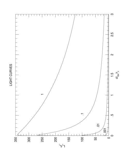
Figure 4: Typical gamma-ray light curves produced by the model for $d/r_{o}>1$. Shown is the total apparent luminosity in units of $L_{j}$, the power of the ejected (fast) outflow, against $ct_{obs}/r_{o}$, $t_{obs}$ being the time measured by distant observer (see text for details). The numbers that label the curves are the values of $(\epsilon L_{s})_{45}/r_{16}$.

The rate of energy dissipation in the front is presented in fig. 3, and it is seen that it increases as the radiated flux increases. The reason is that radiative losses lead to deceleration of the front and shocks (see fig. 1) and, consequently, enhancement in the rate of energy deposition behind the shocks, particularly the reverse shock, as can be inferred from eq. (7). This positive feedback has important implications for the emitted spectrum, particularly in the presence of large pair production opacity, that are discussed below. Fig. 4 depicts typical light curves computed for $d/r_{o}>1$ and different values of $(\epsilon L_{s})_{45}/r_{16}$. In this figure the total apparent gamma-ray luminosity is plotted against the time measured by a distant observer, $t_{obs}=\int_{0}^{t}{[1-\beta_{s+}(t^{\prime})\cos\theta]dt^{\prime}}$, where $\beta_{s+}$ is the velocity of the forward shock, and $\theta$ is the angle to the line of sight ($\theta=0$ in this example). The strong dependence of the flare intensity on the parameter $(\epsilon L_{s})_{45}/r_{16}$ is evident. This is one consequence of the positive feedback mentioned above. The decay of the flare in this regime depends on the radial variation of the intensity of background radiation and the expansion rate of the front, and is typically longer and more gradual than the rise. Further, the rise time increases slightly with increasing $L_{45}/r_{16}$. The reason is that larger opacity results in smaller shock and front velocities during peak emission (see fig. 1) and, therefore, smaller beaming factor. From fig. 4. it is seen that the rise time is of order $(l/2c)\Gamma_{s+}^{-2}(t_{peak})\simeq 10^{-2}r_{o}/c$, where $\Gamma_{s+}(t_{peak})$ is the Lorentz factor of the forward shock near maximum flux, and that the flare duration is several times longer. For $r_{o}$ between 10¹⁵ and 10¹⁸ cm (cf. §2) this corresponds to a rise time in the range between several minutes and several weeks. However, gamma-rays of a given energy cannot escape from a radius smaller than their gamma-spheric radius, so that the duration of a flare in a given band is also limited by the pair production opacity. In general, we find that for parameters typical to the powerful blazars the flare duration in the EGRET band can range from several hours to several weeks for small viewing angles (i.e., $\theta<\Gamma^{-1}$), when $d/r_{o}>1$. The shape of the flare is substantially altered when $d/r_{o}$ becomes sufficiently small. This is demonstrated in Fig. 5 where light curves computed for $L_{45}/r_{16}=1$ and different values of $d/r_{o}$ are displayed. As seen, for values of $d/r_{o}$ smaller than unity the time scale of the flare, as measured by a distant observer, is of order $d/c$; the light curves exhibit a steep decline at times $t_{obs}>d/c$. For sufficiently thin slabs ($d/r_{o}<2\times 10^{-2}$ in this example) the decay time of the flare is comparable to the rise time or even slightly shorter.

In order to examine the relationship between the emergent fluxes in different high-energy bands predicted by our model, we divided the energy interval into several subintervals and followed the time evolution of the flux in each band. Quite generally we find that i) only a relatively small fraction of the radiated energy is emitted above the gamma-spheric energy at which the pair-production optical depth at $r\sim r_{o}+l$ (the front position at peak emission) equals unity, ii) the time of peak emission and flare duration increase with increasing gamma-ray energy in this energy range, and iii) below that energy variations in the fluxes at different X-and gamma-ray bands occurs roughly simultaneously, but not necessarily with the same amplitude. This behavior is also a consequence of the positive feedback discussed above. An example is given in fig. 6, where the time evolution of the energy fluxes emitted in four equally spaced subintervals in the energy interval 5 MeV to 50 GeV, for $d/l>1$ is presented. Similar behavior has been found in the case $d/l<<1$. This result is in contrast with the simultaneous flaring predicted by the model of RL97, which does not take into account gamma-ray attenuation by pair production on external photons.

We also checked the dependence of the front dynamics and emission on the rate of magnetic field dissipation. We find that as $U_{A}$ increases above unity, the front expands more rapidly, adiabatic cooling becomes more important and, hence, the radiative efficiency drops. The rapid expansion results in a slower decay of the flare, but otherwise the shape of the light curve is not altered significantly.

5 Conclusions

This paper considers the production of gamma-ray flares through inverse Compton scattering of external radiation by pairs accelerated behind internal shocks, that are driven by temporal fluctuations in the parameters of a magnetized, relativistic outflow. A self-consistent model capable of describing the dynamics of the front and the time evolution of the angle averaged pair and gamma-ray distribution functions, has been developed and employed to calculate gamma-ray light curves in blazars.

The main results and conclusions of this study are:

1) The shape and timescale of the flare depend on the ratio of the thickness of ejected fluid slab, $d$, and the gradient length scale of the background radiation intensity at the radius of shock formation, $l$. When $d/l$ is sufficiently small, such that the propagation time of the shocks across the fluid slab is shorter than $l/c$, the flare duration, as measured by an observer at small viewing angle, is $\sim d/c$, and the shape of the light curve is roughly symmetric. For larger values of $d/l$ the flare reaches its maximum at a distance $l$ from the creation radius. It then decays gradually until time $d/c$, after which the flux declines steeply. For $d/l>1$ the shape of the flare is determined essentially by the radial variations of the intensity of ambient radiation and the expansion rate of the front; typically, the rise is fast compared with the decay. The above results suggest that different types of flares will be produced in different sources, or even in the same source under different conditions. This expectation appears to be consistent with the variety of types of EGRET flares (e.g., Hartman et al. 1993; Kniffen et al. 1993; Mattox et al. 1997) observed in gamma-ray blazars. In the event of impulsive outflow ejection (i.e., ejection time of order the dynamical time, $\tau_{inj}\simeq\tau_{acc}$; cf. §2) the axial length of the fluid slab can be as small as the size of the central engine. If the latter is associated with the gravitational radius of the putative black hole, $r_{g}$, then flare durations as short as $r_{g}/c\sim 50[M_{BH}/(10^{7}M_{\odot})]$ sec are plausible. Successive ejection of jets with short duty cycle may also lead to a substructure in the light curve of a longer duration outburst (as often seen in GRBs). In general we find that for parameters typical to extragalactic jets, namely $\Gamma$ of order 10 and comoving Alfv́en 4-velocity between 0 and 10, the flare timescale can lie in the range between several minutes and several weeks (for small viewing angles). We note that the shape of the light curve may be significantly altered when the SSC process becomes important (cf. RL97). The study of SSC flares is left for future investigation.

2) The peak flux and flare intensity depend sensitively on the Thomson opacity near $r_{o}$, specifically, on the value of $L_{s}/r_{o}$, where $L_{s}$ is the fraction of nuclear luminosity that is reprocessed or scattered across the jet. This behavior is a consequence of a positive feedback that gives rise to a strong enhancement of the energy deposition rate during peak emission. For parameters typical to the powerful gamma-ray blazars, the radiative efficiency, namely the fraction of dissipation energy that is radiated by the front is typically high ($>60\%$).

3) The amplitude of variations of the flux emitted at energies for which the pair-production optical depth is initially larger than unity is much smaller than that at lower energies. The flare, in this energy interval, propagates from low to high energies and its duration increases with energy. At lower energies, flaring in different X-and gamma-ray bands occurs roughly simultaneously, but with possibly different amplitudes, depending on the spectra of ambient radiation and injected electrons. The claimed invariance of the gamma-ray spectrum during the strong EGRET flare observed in PKS1622-297 (Mattox et al. 1997) is not in conflict with that model prediction, since the sensitivity was insufficient to resolve any time lags, if present, between the fluxes in the two energy subintervals (below and above 300 MeV) analyzed by those authors, particularly in view of the small amplitudes anticipated at high EGRET energies. Despite the small amplitudes, it may be possible to observe time lags between the emission at hard (but still well below TeV where absorption by the IR background is strong) and soft gamma-ray energies with a next generation gamma-ray telescope. The detection of such lags is an important test for this model. One implication of the above results is that in some cases strong flares may be observed in some energy bands while the simultaneous variations in other bands may appear modest or even small. The simultaneous X-ray/TeV flare reported recently for Mrk 421 and the lack of significant variations of the EGRET flux (Macomb, et al. 1995; Takahashi et al. 1996) is an example. The hard X-ray flux may be due to either inverse Compton emission of the thermal electrons or synchrotron emission of the highest energy electrons. Alternatively, this event may be explained as an SSC flare resulting from changes in the tail of the distribution of non-thermal electrons (Takahashi et al. 1996).

I thank the referee, R.V.E. Lovelace, for useful comments. Support by Alon fellowship and a TAU Research Authority grant is acknowledged.

Appendix A Appendix: Derivation of the front equations

Equations (4) are of the form,

$$\partial_{\mu}A^{\mu}=B.$$ (A1)

Integrating the above equation over a region in space-time enclosed by the world lines associated with the left shock, the contact discontinuity and the lines defined by the equations $t=t_{o}$; $t=t_{o}+\Delta t$, where $t_{o}$ is some fiducial time [see fig. (7)] , and using the generalized Gauss’s theorem,

$$\int{A^{\mu}d^{3}\Sigma_{\mu}}=\int{Bd^{4}\Omega},$$ (A2)

where $d^{4}\Omega$ is a volume element and $d^{3}\Sigma_{\mu}$ is the surface area of the 3d surface enclosing the region of integration yields,

$$\int_{t_{o}}^{t_{o}+\Delta t}{\{A^{o}_{-}\beta_{s-}-A^{x}_{-}+A^{x}_{f-}(x_{c})-A^{o}_{f-}(x_{c})\beta_{c}\}cdt}+\int_{x_{c}(t_{o})}^{x_{-}(t_{o})}{A^{o}_{f-}(t_{o})dx}$$

$$-\int_{x_{c}(t_{o}+\Delta t)}^{x_{-}(t_{o}+\Delta t)}{A^{o}_{f-}(t_{o}+\Delta t)dx}=\int_{t_{o}}^{t_{o}+\Delta t}{cdt\int_{x_{c}(t)}^{x_{-}(t)}{B(t)dx}},$$ (A3)

where it has been assumed that $A^{\mu}$ and $B$ depend solely on the axial coordinate (i.e., along the direction of motion). In the limit $\Delta t\rightarrow 0$, and using the expansions $x_{c}(t_{o}+dt)\simeq x_{c}(t_{o})+\beta_{c}(t_{o})dt$; $x_{-}(t_{o}+dt)\simeq x_{-}(t_{o})+\beta_{s-}(t_{o})dt$, we arrive at,

$$A^{o}_{-}\beta_{s-}-A^{x}_{-}-A^{o}_{f-}(x_{-})\beta_{s-}+A^{x}_{f-}(x_{c})+\int_{x_{-}}^{x_{c}}{\frac{\partial A_{f-}^{o}}{c\partial t}dx}-\int_{x_{-}}^{x_{c}}{B_{-}dx}=0.$$ (A4)

Likewise, integrating eq. (A1) over a portion of space time containing the region rightward to the contact discontinuity yields,

$$-A^{o}_{+}\beta_{s+}+A^{x}_{+}+A^{o}_{f+}(x_{+})\beta_{s+}-A^{x}_{f+}(x_{c})+\int_{x_{c}}^{x_{+}}{\frac{\partial A_{f+}^{o}}{c\partial t}dx}-\int_{x_{c}}^{x_{+}}{B_{+}dx}=0.$$ (A5)

Under the assumption that $A_{f\pm}$ are homogeneous inside the front, (i.e., independent of the axial coordinate x, but may still have different values on each side of the contact discontinuity), we obtain the following differential equations for $A_{f\pm}(t)$

$$\pm(\Delta X_{\pm})^{-1}(A^{o}_{\pm}\beta_{s\pm}-A^{x}_{\pm}-A^{o}_{f\pm}\beta_{s\pm}+A^{x}_{f\pm})-\frac{\partial A_{f\pm}^{o}}{\partial x^{o}}+B_{\pm}=0,$$ (A6)

where $\Delta X_{\pm}(t)=\pm\int_{x_{c}(t)}^{x_{\pm}(t)}{dx}$ is the distance between the forward (reverse) shock and the contact discontinuity.

Substituting the front quantities for $A^{\mu}$ one obtains,

$$\pm[N_{f\pm}(\beta_{s\pm}-\beta_{c})-N_{\pm}(\beta_{s\pm}-\beta_{\pm})]+\Delta X_{\pm}\left(\frac{\partial N_{f\pm}}{\partial x^{o}}-Q_{\pm}\right)=0,$$

$$\pm[B_{f\pm}(\beta_{s\pm}-\beta_{c})-B_{\pm}(\beta_{s\pm}-\beta_{\pm})]+\Delta X_{\pm}\left(\frac{\partial B_{f\pm}}{\partial x^{o}}-Q_{b\pm}\right)=0,$$ (A7)

$$\pm[(T^{00}_{f\pm}\beta_{s\pm}-T^{0x}_{f\pm})-(T^{00}_{\pm}\beta_{s\pm}-T^{0x}_{\pm})]+\Delta X_{\pm}\left(\frac{\partial T^{00}_{f\pm}}{\partial x^{o}}-S^{0}_{\pm}\right)=0,$$

$$\pm[(T^{0x}_{f\pm}\beta_{s\pm}-T^{xx}_{f\pm})-(T^{0x}_{\pm}\beta_{s\pm}-T^{xx}_{\pm})]+\Delta X_{\pm}\left(\frac{\partial T^{0x}_{f\pm}}{\partial x^{o}}-S^{x}_{\pm}\right)=0.$$

Here $B_{f\pm}=b_{f\pm}\gamma_{c}$ is the magnetic field as measured in the injection frame, $\beta_{s\pm}$ are the corresponding shock velocities, and $\beta_{c}$ is the velocity of the contact discontinuity.

Figure 1: Time evolution of front quantities. Shown are (a) the 4-velocity of the contact discontinuity (labeled $U_{c}$), forward shock (labeled $U_{s+}$) and reverse shock (labeled $U_{-}$), (b) the proper density, (c) the total pressure, and (d) magnetic pressure as a function of ln($ct/r_{o}$), for $(\epsilon L_{s})_{45}/r_{16}=1$ (solid line) and $10^{-2}$ (dotted line). Here $(\epsilon L_{s})_{45}$ is the fraction of ambient luminosity scattered across the jet in units of $10^{45}$ ergs s^-1, and $r_{16}$ is the radius of shock formation in units of 10¹⁶ cm.

Figure 2: Radiative efficiency, defined as the fraction of dissipation power radiated by the front (see text), versus log of injection frame time.

Figure 3: Time evolution of the dissipation power. The dissipation flux is normalized to the bulk energy flux of the fast fluid. Curves are labeled by values of log[$(\epsilon L_{s})_{45}/r_{16}$]

Figure 5: The same as fig. 4, but for $(\epsilon L_{s})_{45}/r_{16}=1$ and different values of $d/r_{o}$ (label the curves).

Figure 6: Spectral evolution: displayed are the total apparent luminosities in four equally spaced energy intervals in the range 5 MeV to 50 GeV (indicated in window a; energies are given in units of GeV), for $d/r_{o}>1$ and (a) $(\epsilon L_{s})_{45}/r_{16}=1$, (b) $(\epsilon L_{s})_{45}/r_{16}=10^{-1}$, (c) , $(\epsilon L_{s})_{45}/r_{16}=10^{-2}$ and (d) $(\epsilon L_{s})_{45}/r_{16}=10^{-3}$.

Figure 7: Schematic diagram showing the world-lines of the forward shock ($\beta_{+}$), reverse shock ($\beta_{-}$), and the contact discontinuity ($\beta_{c}$), and the corresponding contours of integration (dashed lines). The region marked by the minus (plus) sign corresponds to the portion of the front leftward (rightward) of the contact discontinuity surface.

References

- (1) Blandford R.D., & Levinson, A. 1995, ApJ, 441, 79 (BL95)
- (2) Bloom, S.D., & Marscher, A.P. 1993, in Compton Gamma-Ray Observato ry, ed. N. Gehrels (New York: AIP), pp. 578
- (3) Buckley, HH. et al. 1996, A&A, 472, L9
- (4) Burns, M.L., & Lovelace R.V.E. 1982, ApJ, 262, 87
- (5) Dermer, C., & Schlickheiser, R. 1993, ApJ, 416, 458
- (6) Ghisellini, G., & Madau, P. 1996, MNRAS., 280, 67
- (7) Hartman, R.C., et al. 1993, ApJ, 407, L41
- (8) Levinson A., & Blandford, R.D. 1995, ApJ, 449, 86
- (9) Levinson, A. 1996, ApJ, 467, 546
- (10) Levinson, A. & Van Putten, M.V.P. 1997, ApJ, 488, 69
- (11) Macomb, D.J., et al. 1995, ApJ, 449, L99
- (12) Mannheim, K. 1993, A&A, 269, 67
- (13) Maraschi, L. et al. 1994, ApJ, 435, L91
- (14) Mattox, J., et al. 1997, ApJ, 476, 692
- (15) Raga, A.C., et al. 1990, ApJ, 364, 601
- (16) Reich, W., et al. 1993, A&A, 273, 65
- (17) Romanova, M.M., & Lovelace, R.V.E. 1992, A&A, 262, 26
- (18) Romanova, M.M., & Lovelace, R.V.E. 1997, ApJ, 475, 97 (RL97)
- (19) Sambruna, R.M., et al. 1997, ApJ, 474, 639
- (20) Sikora, M., Begelman, M., & Rees, M. 1994, Astrophys. J. 421, 153
- (21) Sikora, M., et al. 1997, preprint
- (22) Takahashi, T., et al. 1996, ApJ., 470, L89
- (23) Thompson, C. 1997, in Relativisitic Jets in AGN, eds. M. Ostr owski, M. Sikora, G. Madejski & M. Begelman, in press
- (24) Ulrich, M., Maraschi, L., & Urry, M.C. 1997, ARA&A, 35, 445
- (25) Wagner, S.J. 1996, ApJS., 120, 495
- (26) Wehrle, A.R., et al. 1997, ApJ., in press