Radiative Transfer Modelling of the Accretion Flow onto a Star-Forming Core in W51

Abstract

We present an analysis of the temperature, density, and velocity of the molecular gas in the star-forming core around W51 e2. A previous paper (Ho & Young 1996) describes the kinematic evidence which implies that the core around e2 is contracting onto a young massive star. The current paper presents a technique for modelling the three-dimensional structure of the core by simulating spectral line images of the source and comparing those images to observed data. The primary conclusions of this work are that the molecular gas in e2 is radially contracting at about 5 km s^-1 and that the temperature and density of the gas decrease outward over 0.15 pc scales. The simple model of the collapse of the singular isothermal sphere for low-mass star formation (Shu 1977) is an inadequate description of this high-mass molecular core; better models have temperature $\propto r^{-0.6}$, density $\propto r^{-2}$, and velocity $\propto r^{+0.1}$. The core appears to be spherical rather than disk-like at the scale of these observations, 0.3 pc. In this paper we show how a series of models of gradually increasing complexity can be used to investigate the sensitivity of the model to its parameters. Major sources of uncertainty for this method and this dataset are the interdependence of temperature and density, the assumed $\rm NH_{3}$ abundance, the distance uncertainty, and flux calibration of the data.

1 Introduction

In recent years, radio interferometric telescopes have provided a wealth of data on the internal structure and dynamics of molecular clouds and star forming regions on scales of 1 pc and smaller. For example, observations of neutral gas have shown the presence of infall and spin-up motions, rotating disks, outflows, and expanding molecular shells at later stages in the formation of stars (Ho & Haschick 1986; Keto, Ho, & Haschick 1987, 1988; Torrelles et al. 1989; Sargent & Beckwith 1991; Carral & Welch 1992; Torrelles et al. 1993; Kawabe et al. 1993; and Ho & Young 1996, hereafter Paper I). The details of the collapse process are vital to understanding how stars can be formed– how angular momentum and magnetic flux are transported out and how simultaneous accretion and outflow determine the mass of the resultant star.

Theoretical models have mostly focused on the formation of low-mass stars. For example, Shu (1977) analyzed the gravitational collapse of non-rotating, non-magnetic, isothermal gas spheres. He proposed an “inside-out” collapse in which the contracting portions of the cloud should develop an $r^{-1.5}$ density profile and an $r^{-0.5}$ radial infall velocity. More recently, Mouschovias and others considered the effects of magnetic fields; they found that under certain common conditions the density will vary as $r^{-1.5}$ to $r^{-2}$ over scales of 10^-3 pc to a few tenths of a parsec (e.g. Basu & Mouschovias 1994). Scoville & Kwan (1976) studied the temperature distribution in a centrally condensed cloud heated by a source of radiation such as an HII region. Assuming thermal equilibrium between the radiation and the dust, and between the dust and the gas, they calculate that the temperature of the gas and dust should decrease with radius as $r^{-0.3}$ or $r^{-0.4}$. They expect to find temperatures of 50–70 K at a distance of 0.07 pc from an object of luminosity 10⁵ $\rm L_{\sun}$, given typical gas and dust conditions. The present paper is part of a study to observationally measure some basic properties of high-mass star formation and to determine whether the results mentioned above, some of which are intended for low-mass stars, also describe high-mass star formation.

Paper I presents observations of the $\rm NH_{3}$ (J,K) = (2,2) 24 GHz inversion transitions in the star forming region W51. Those observations detected an accretion flow of a few km s^-1, extending over about 0.3 pc in diameter, onto a young star. The star must be massive because it has created an ultracompact HII region, called W51 e2, which is embedded in the molecular core. The current paper takes a numerical modelling approach to finding the structure of the star forming core in W51. Paper I’s observations of W51 e2 are compared with theoretical spectra that would be observed from a model with a specified temperature, density, and velocity structure. We begin with the simplest model with the fewest parameters, that of a uniform density isothermal sphere, and show how the addition of an infall velocity and temperature and density gradients improves the fit to the data. This approach constrains the physical conditions of the molecular gas in the core; it also has the important advantage of revealing how tightly the present data and models can constrain those conditions.

2 Background

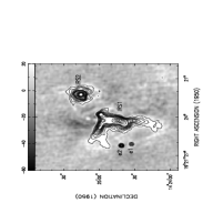
Figure 1: Continuum emission at 1.3 cm from W51, taken from Paper 1. Contour levels are (1, 2, 3, 4, 5, 6, 7, 8, 9, 10, 15, 20, 25, 30, 35, 40, 45, 50, 100) $\times$ 20 mJy/beam or 6.4 K. The greyscale image is also the continuum emission from 20 mJy/beam to $-$60 mJy/beam as shown in the scale at top. The resolution is 2.6″.

W51 is an active region of high mass star formation, as shown by its large luminosity (3$\times 10^{6}$ $\rm L_{\sun}$, Thronson & Harper 1979), IR objects (Genzel et al. 1982; Bally et al. 1987), H₂O masers (Schneps et al. 1981), and shocked $\rm H_{2}$ emission (Beckwith & Zuckerman 1982). Genzel et al. (1981) used the method of statistical parallax of H₂O masers around the HII region W51 e2 (Scott 1978) to determine a distance of 7.0$\pm$1.5 kpc, and similar distances have been found for the other objects in the W51 complex. This paper concerns the ultracompact HII region W51 e2 and the molecular core surrounding it. Figure 1 shows the 1.3 cm continuum emission in W51. Scott (1978) noted that the flux from the HII region in e2 could be accounted for by the presence of one ZAMS star of spectral type B0–O9. HII regions e1 and e2 also are surrounded by condensations of warm $\rm NH_{3}$, detected in both emission and absorption by Ho, Genzel, & Das (1983). Though outflows are seen in other parts of the W51 complex, there is little evidence of outflow activity near the e2 core on the arcsecond scales of interest here (Mehringer 1994; Zhang & Ho 1997).

2.1 Data

The observations for Paper I and the data reduction techniques used are described in detail in that paper. Briefly, we used the NRAO Very Large Array (VLA) to observe the $\rm NH_{3}$ (J,K) = (1,1) and (2,2) inversion transitions at 23.69 GHz and 23.72 GHz. The bandwidth of 6.25 MHz covers the main quadrupole hyperfine component and all four satellite components with 64 velocity channels. The velocity resolution of this data is 1.24 km s^-1, and the bandpass was centered on a velocity of +60 km s^-1 with respect to the local standard of rest (LSR). The images studied in this paper were made with a spatial resolution (FWHM) of 2.6″, or 0.09 pc at a distance of 7.0 kpc. The rms noise level in the line-free channels is 6 mJy/beam = 1.9 K.

2.2 Prediction of geometry in the core e2

Figure 2 presents a position-velocity diagram made along a slice through the e2 molecular core; the models of this paper attempt to reproduce the features shown in this diagram. (Paper I presents many additional figures showing the distribution and velocity structure of the molecular gas in and around W51 e2.) A good model of the molecular gas in the e2 core should reproduce the following features which are visible in Figure 2 and in the figures of Paper I.

1. The five hyperfine components of the transition are visible in both emission and absorption because the absorption is consistently redshifted with respect to the emission. The absorption corresponds to cool (relative to the HII region) molecular gas in front of the HII region, whereas molecular gas to the side or in back of the HII region is in emission.

2. The central hyperfine component of the emission line in e2 shows a curvy “C” shape. Emission east and west of the HII region (upper and lower edges of the panel; see also Paper I) is at a velocity of about 55 km s^-1. Towards the center of the panel (the center of the HII region and molecular core) the emission line becomes more blueshifted. The line center and systemic velocity of the core seem to be at 54–55 km s^-1, which is about halfway between the emission and absorption, at 50 and 60 km s^-1 respectively.

3. The “C” shape appears in any position-velocity diagram that is made through the core e2, regardless of orientation. Thus, position-velocity diagrams through e2 show approximate circular symmetry on the sky.

4. The position-velocity diagrams that just miss the HII region (see Paper I) do not show absorption or a curved C-shaped emission line, but they do show that the lines are wider at the position of the HII region than, for example, east or west of it. In other words, this feature is an increase in line width at small spatial scales.

5. Optical depths in the (2,2) transition in e2 are high; the ratio of the central hyperfine emission component to the satellites is 2.5:1 to 3:1 in the core (Paper I), implying emission optical depths of 7–10 (Ho & Townes 1983). In absorption all five hyperfine components have approximately the same strength, implying very high optical depth.

6. In e2 the peak of emission and the peak of absorption are not spatially coincident, as might be expected for a perfectly spherically symmetric core. Instead the emission and absorption peaks are offset by 3″ or 0.1 pc, suggesting that the HII region is off-center with respect to the molecular gas or that the properties of the gas are not spherically symmetric. This offset is confirmed by higher resolution observations (Zhang & Ho 1997).

Paper I proposes a simple explanation, summarized here, that explains these observed features. The molecular core e2, about 0.13 pc in radius, is a roughly spherical cloud of gas which is contracting onto a young massive star and HII region near the center of the sphere. Thus the front of the cloud is moving away from us and the back is moving toward us, as required by the redshifted absorption and blueshifted emission; the “C” shape is a projection effect. The assumption of a roughly spherical contraction explains the approximate circular symmetry in the plane of the sky (point 3 above). Paper I discusses this interpretation in more detail.

3 Procedure

We investigate the structure of the molecular core around e2 by radiative transfer modelling of the $\rm NH_{3}$ emission. Because the data show approximate circular symmetry in the plane of the sky (Section 2.2), we modelled only one two-dimensional slice, or position-velocity diagram, through the e2 core. Figure 2 is the position-velocity diagram selected for modelling; it is the (J,K) = (2,2) transition, and passes through the center of the HII region. Figure 2 shows many of the features described in Section 2.2. The data in Figure 2 were spatially subsampled by taking five pixels separated by the FWHM of the beam, and were trimmed in velocity by selecting the central 50 of the observed 64 velocity channels. The result of the subsampling is shown in the top left panel of Figure 3; it is made up of 250 independent data points.

The radiative transfer code used in our spectral line modelling is described briefly in Keto (1990). Based on Paper I’s discussion of physical conditions in e2, we determined an initial guess of the structure— temperature, density, and velocity field— of the core. For simplicity, the physical parameters are described as power-law parametrizations in radius. Level populations of $\rm NH_{3}$ are determined using the assumption of local thermodynamic equilibrium (LTE), and the line brightness is computed by integrating the radiative transfer equation along the line of sight. The calculated line radiation is convolved to the resolution of the observed data and converted to the same physical units as the observed data. Thus the models in Figures 3 and 4 are sampled at the same spatial frequency as the data in the top left panel of Figure 3, and their intensities are directly comparable.

In addition, we have added for this project a least squares fitting procedure to optimize the modelled physical conditions. The multidimensional least-squares fit is done using a downhill simplex algorithm (Press et al. 1993). This algorithm is a gradient descent procedure which reaches a local minimum but not necessarily a global minimum. The fitting routine imposes no constraints on “reasonable” or “acceptable” physical conditions or power-law slopes aside from the requirements that gas temperatures exceed 3 K and densities exceed 10 $\rm cm^{-3}$. Energetic and dynamic consistency of the models are considered in Section 5.1.

The radiative transfer/model fitting code also performs a simple error analysis. It estimates the error in each parameter as the second derivative of $\chi^{2}$ with respect to the parameter using the values of $\chi^{2}$ at the optimized value of the parameter and at two symmetrically offset values of the parameter (Bevington, 1969). This procedure for estimating the error assumes that the parameters are uncorrelated and that the model is linearly dependent on them. Neither of these conditions are true; however, comparison with a limited Monte Carlo analysis indicates that our derived errors are at least of the correct magnitude.

Subsequent sections present the results of the data fitting for the molecular core e2, employing a series of models of gradually increasing complexity. For example, the first model is a spherical cloud of molecular gas of constant temperature and density and an HII region inside. In successive models, parameters allowing for infall velocity and for gradients in the temperature, density, and velocity are added. There is no evidence for rotation in e2 on the scales of interest here (Paper I), so the models do not include rotation. (Zhang & Ho [1997] found evidence of spin-up in e2 but only at radii less than 0.2″, much smaller than the 1.3″ resolution used for the current study.) The technique of gradually increasing the complexity of the models proves extremely valuable because comparisons between the models reveal (1) which parameters are important and which are not; (2) how well determined are the physical conditions in the core.

4 Results

4.1 Model 1: quiescent cloud

The first model consists of an HII region surrounded by a spherical cloud of molecular gas with uniform density and temperature, and no infall velocity. A turbulent line width (FWHM) of 1.25 km s^-1 in the molecular gas is assumed, based on the observed line width in an optically thin envelope of gas surrounding e2 and e1 (Paper I). We also assume a fractional abundance $\rm NH_{3}$/$\rm H_{2}$ = 1.4$\times 10^{-6}$ in order to translate from the $\rm NH_{3}$ density, which is constrained by the data, to the $\rm H_{2}$ densities quoted in this paper. This $\rm NH_{3}$ abundance is based on modelling of a similar high-mass star formation region, G10.6–0.4 (Keto, Ho, & Haschick 1988). Abundances around 10^-6 are also estimated for the $\rm NH_{3}$ near G9.62+0.19 and G29.96–0.02 (Cesaroni et al. 1994). The turbulent line width and $\rm NH_{3}$ abundance remain fixed for all models. Model 1 has six free parameters: the systemic velocity of the HII region, the continuum opacity of the HII region, the radius of the HII region (taken to be the inner radius of the molecular gas), the outer radius of the molecular cloud, and the temperature and density of the gas in the cloud. This model provides a null hypothesis for comparison to models with contracting molecular gas.

Table 1 gives the initial guesses of the parameters describing the gas in this and subsequent models; Table 2 gives the optimized parameters and reduced $\chi^{2}$ (per degree of freedom) for all models. The initial guesses are presented because the more complicated models sometimes give substantially different output from different sets of initial conditions; this issue is discussed more fully in Section 4.4. Table 3 also gives maximum and minimum values for the gas temperature, density, and velocity.

Figure 3 presents the best fit position-velocity diagram for model 1 and subsequent models. The panel labelled “1” should be compared to the data in the top left panel of the same figure. The most obvious problem with this model is that because infall (or outflow) is not allowed, emission and absorption are constrained to have the same line width and same radial velocity. In this fit, the radius and continuum opacity of the HII region are consistent with zero: 0.003$\pm$0.06 pc and (0.02$\pm$3)$\times 10^{-19}$ $\rm cm^{-1}$. The fitted optical depth of the HII region is only 3$\times 10^{-5}$, so low that absorption is not seen. The value of the reduced $\chi^{2}$ (per degree of freedom) for this model is 11.2, which is little better than the $\chi^{2}$ of blank sky (12.2).

4.2 Model 2: contracting cloud with uniform temperature and density

The second model incorporates all the features of the first model, namely an HII region surrounded by a spherical cloud of gas with uniform temperature and density, and adds a radial infall velocity of the form $v=v_{0}(r/{r_{0}})^{\alpha_{v}}$. Model 2 fits eight free parameters: $v_{0}$, $\alpha_{v}$, and the six parameters of model 1.

Again, Figure 3 and Table 2 present the results of this optimization. Clearly, the addition of infall velocity improves the model immensely. The value of reduced $\chi^{2}$ drops by almost a factor of three, to 3.8. The fitted continuum opacity of model 2 is 1.4$\times 10^{-19}$ $\rm cm^{-1}$, producing a continuum optical depth of 0.02 for the HII region. (Subsequent models have very similar continuum optical depths. However, we caution that these continuum parameters are poorly constrained because the HII region is not resolved by these observations; see Gaume, Johnston, & Wilson 1993.) In contrast to model 1, the gas in front of the HII region is now redshifted and is seen in absorption. The pattern of redshifted absorption and blueshifted emission, so obvious in the data, is now reproduced by the model as well.

4.3 Model 3: Shu (1977)

The simple analytic solution of Shu (1977) for the properties of a collapsing molecular core can be directly tested using our observations of W51 e2. Since that analytic solution was developed specifically for the case of low mass star formation, the relevance of the solution for the e2 core is not obvious. However, the Shu (1977) solution is included as model 3 because comparisons between model 3 and models 2, 4a, and 4b help disentangle the importance of the various parameters. Model 3 is similar to model 2 except for the addition of a radial gradient in density, fixed as $n\propto r^{-1.5}$. In addition, the infall velocity is fixed at $v\propto r^{-0.5}$, and there is no gradient in temperature. Thus, model 3 has seven free parameters: the eight of model 2, minus the slope describing the gradient in infall velocity.

The minimized value of reduced $\chi^{2}$ for model 3 is greater than that for model 2 by 0.3. As for model 2, also an isothermal model, the emission main/satellite hyperfine intensity ratio is too low and the emission is not strong enough, which would be rectified by the addition of some hotter and optically thinner molecular gas. Thus Shu’s low-mass stellar collapse model is not an adequate description of the collapse of the high-mass e2 molecular core. An obvious reason is the increased importance of central heating in the high-mass case. Subsequent models return to fitting the density, velocity, and temperature slopes as free parameters.

4.4 Model 4: gradients in temperature and density

Model 4 incorporates the features of model 2 and adds radial gradients in temperature and density. Radial gradients are expected to improve the fit to the data for the following empirical reason. The data (Figure 2) show stronger emission in the main hyperfine component than in the satellites, whereas models 2 and 3 produce about the same intensity in all emission components. Density and temperature gradients allow the introduction of some hotter, optically thinner gas, which would increase the relative strength of the central hyperfine component. Model 4 has 10 free parameters: the same eight as model 2, plus the exponents in the temperature and density power laws.

Table 2 presents the results of two optimizations of model 4, and the corresponding position-velocity diagrams are both presented in Figure 3. The difference between model 4a and model 4b is simply the initial guess (Table 1); model 4a starts with a higher density and a lower temperature than model 4b. The reason for running these two cases is that we know the brightness of a single molecular line cannot be used to uniquely determine both the gas temperature and density. In the optically thin case, for example, the line brightness temperature is the product of the temperature and optical depth. Thus, the two different models 4a and 4b allow us to gauge how well temperature and density can be constrained. Both models 4a and 4b are significant improvements over the models 2 and 3; their values of reduced $\chi^{2}$ are 3.2 and 3.0, respectively, compared to 3.8 for model 2 and 4.1 for model 3. The difference in $\chi^{2}$ between 3.2 and 3.0 is not significant.

The optimized infall velocities are not very different in models 4a and 4b from the infall velocities in model 2 (Table 3), which implies that the infall velocities are well constrained in this technique. Comparing models 4a and 4b to models 2 and 3, the central emission components are stronger and the main/satellite intensity ratios are higher. The emission also has a larger spatial extent in models 4a and 4b than in model 2. In the optimized models 4a and 4b, molecular gas densities drop by two orders of magnitude between the outer radius of the HII region and the outer radius of the cloud; the temperatures drop by about 10–15 degrees. Thus, a good description of the core e2 requires radial gradients (decreasing outwards) in temperature and/or density. Model 3, which is isothermal but has a density gradient, suggests that a radial gradient in density alone is not sufficient for a model of e2; a gradient in temperature is also required. Of course, a temperature gradient should not be surprising since there is a heat source (the star) in the center of the core. Analysis of the low-mass star-forming core B335 (Zhou et al. 1993) also shows evidence for a temperature gradient in that core.

As expected, the results of models 4a and 4b show that the temperature and density are not independent parameters; to some extent, a lower temperature can be compensated by a higher density. Fitting two $\rm NH_{3}$ transitions simultaneously, such as (1,1) and (2,2), would remove this ambiguity. Uncertainties are discussed further in Section 5.3.

4.5 Models 5a and 5b: offset HII region

The modest asymmetries in the observed $\rm NH_{3}$ emission suggested that a better fit to the data might be achieved by displacing the HII region a few arcseconds (up to 0.1 pc) from the center of the spherical molecular core (Section 2.2). Models 5a and 5b elaborate on models 4a and 4b by including the position of the HII region within the core as free parameters. The molecular gas temperature is calculated with respect to distance from the HII region, the heat source. Density and infall velocity are calculated with respect to distance from the center of the spherical core, as the young star’s mass is much less than the mass of molecular gas in the core (Paper I; Zhang & Ho 1997). This rather simplistic model has the advantage that it introduces some asymmetry without adding many new free parameters. Models 5a and 5b have twelve free parameters: the same ten from models 4a and 4b, with the addition of the HII region’s offset in two directions (along the line of sight and the direction of right ascension).

As for models 4a and 4b, models 5a and 5b differ in their initial guess parameters. The results of these optimizations are given in Figure 4 and in Table 2. For model 5a, the initial guess offset of the HII region is 0 pc, and for model 5b the initial offsets are 0.05 pc in each of the two directions, chosen to agree with the asymmetries in the data. Neither the optimized model 5a nor 5b achieves a significant improvement in reduced $\chi^{2}$ over models 4a and 4b. Model 5b better matches the east-west asymmetry of the data. However, in both models 5a and 5b the optimized offsets are not significantly different from the initial guesses. It is possibile that our downhill simplex procedure failed to optimize this particular model, despite its success with the others. More likely, this result suggests that the model of the HII region offset from the center of its parent accreting cloud is not correct in the case of e2. The asymmetry might be better described by a different model. For example, there could be an overall east-west density gradient in the molecular core around e2. Another possibility is that the molecular core might not be spherical; we explore this possibility in models 6a and 6b.

4.6 Models 6a and 6b: molecular disk

Because a non-spherical cloud model might help reproduce some of the east-west asymmetry in the observations of e2, models 6a and 6b describe the molecular gas in e2 as a disk rather than a sphere. The disk is simply an oblate spheroid whose unique axis is confined to lie somewhere between the line of sight and the right ascension axis (the direction of the position-velocity diagram). Since only one position-velocity diagram is modelled, only one inclination angle is required to specify a unique orientation of the disk. Models 6a and 6b have 12 free parameters: the same 10 from models 4a and 4b, with the addition of the axial ratio of the spheroid and the inclination angle. The position of the HII region is fixed at the center of the disk. No constraints are placed on the axial ratio or inclination of the disk, but the approximate observed circular symmetry (Section 2.2) implies that a highly inclined thin disk is an unreasonable solution.

Again, the two disk models 6a and 6b differ in their initial guess parameters. Model 6a had an initial aspect ratio of 1:1, and its optimized parameters are quite similar to those of models 4a and 5a. Model 6b started with an aspect ratio of 4:1 and an inclination of 45° (0° is face-on); its result is a flat disk (10:1), with an inclination of 0°. Figure 4 shows that model 6b does the best job of all models in reproducing the large spatial extent of the central emission component. Model 6b also has the highest central-to-satellite intensity ratio in emission, which probably results from the relatively high temperatures in this model (Table 3; Section 5.2). However, neither model 6a nor 6b has significantly lower $\chi^{2}$ than the simpler models 4a and 4b or the offset HII region models 5a and 5b. Furthermore, as in the case of the offset HII region, the two disk models do not converge to the same result. These facts suggest that the aspect ratio and inclination of any putative disk structure are not well constrained by the current procedure.

On the philosophy that we should adopt the simplest model which best describes the data, we plot reduced $\chi^{2}$ against the number of parameters in each model (Figure 5). This figure shows that as parameters are added, the fit of the models to the data improves until model 4 is reached. Models 5 and 6 increase the complexity of the model without significantly improving the fit to the data. Nevertheless, there are still a number of features of the data which are not reproduced by the models (Section 5.2). We infer that the e2 core cannot be described as a simple sphere, but the specific asymmetries described by models 5 and 6 are not required nor ruled out by the data. We should therefore base our conclusions on model 4, which requires the presence of infall and a centrally condensed and centrally heated molecular core.

4.7 Quantitative results

Most of the optimized density exponents are close to $n\propto r^{-2}$. This slope is steeper than most theoretical predictions for low-mass stars, which give $n\propto r^{-1.5}$ within the region of contraction (e.g. Shu 1977). However, a slope of $-$2 also agrees with the empirical results of Zhang & Ho (1997) for the W51 e2 core. They used higher resolution VLA observations to fit the column density of $\rm NH_{3}$ versus radius in e2 and find $n\propto r^{-2.0^{+}_{-}0.1}$ within 5″ (0.2 pc) of the HII region. This agreement between the empirical results and radiative transfer modelling gives additional confidence in the modelling technique. Of course, the model results are based on the assumptions of LTE and constant $\rm NH_{3}$ abundance. Uncertainties introduced by these assumptions are discussed further in Section 5.3.

There are two models with density slopes quite different from $-$2. In model 4b the density falls off quite steeply ($r^{-3.9}$), which might be due to a trade-off between its high temperatures (relative to the other models) and density. In model 5b the density increases with larger radii ($r^{+0.9}$), which is dynamically unstable and physically unrealistic. This unusual result probably comes from calculating the density with respect to the center of the sphere whereas the HII region is in fact offset by 0.07 pc from that center in this model.

The radiative transfer models also have the temperature falling off a bit more steeply than expected. Models 4a, 5a, 5b, 6a, and 6b have $T\propto r^{-0.6}$, whereas Scoville & Kwan (1976) predicted $T\propto r^{-0.4}$. In contrast, Zhang & Ho (1997) find no evidence of temperature gradients in the central 5″ (0.2 pc) of the e2 molecular core. Formal errors for the temperature exponent (see Table 2) are consistently close to 0.05. However, those formal errors are most likely an underestimate of the true uncertainties (Section 5.3), so the temperature gradients in e2 may be consistent with theoretical models. Since the isothermal models (numbers 2 and 3) have significantly higher $\chi^{2}$ than those that fit a temperature gradient, we conclude that an isothermal model is firmly ruled out by the radiative transfer fitting technique. It is not clear why this modelling should give a different slope than Zhang & Ho (1997) find, except perhaps for the fact that their result is based on line ratios whereas the current technique uses essentially the beam-diluted brightness temperature.

Those models which fit an infall velocity gradient have slopes between $v\propto r^{0.2}$ and $v\propto r^{0}$. Even models 2, 4a, and 6a, whose initial slope was $-0.5$, have optimized slopes greater than zero. Those slopes are not consistent with the “inside-out” scenario proposed by Shu (1977), in which the infall velocity must decrease with increasing radius. In a different star-forming core, however, an inside-out collapse has been inferred. In G10.6–0.4, the infall velocity decreases with radius at least as quickly as $v\propto r^{-0.5}$ (Keto, Ho, & Haschick 1988). If an inside-out, accelerating collapse were present in W51 e2 as well, we would expect to observe higher velocities on smaller spatial scales— at least 10 km s^-1 at the 0.01 pc scales observed by Zhang & Ho (1997). However, such high velocities are not observed. This result could be related to the fact that the HII region is actually offset from the center of the molecular core.

Table 3 presents maximum and minimum values of the temperature, density, and infall velocity in each model, as well as the total gas mass. The extrema are calculated at the inner and outer edges of the shell of molecular gas, as appropriate for each model. From this table we see that the models all have infall velocities of 4–6 km s^-1, which are consistent with the value inferred in Paper I. Such velocities are about a factor of 10 higher than the isothermal sound speed (0.5 km s^-1 for molecular hydrogen at 50 K). Basu & Mouschovias (1994, 1995) have theoretically analyzed the collapse of magnetized molecular cloud cores with ambipolar diffusion, and they predict infall velocities close to the sound speed, rather than an order of magnitude higher than the sound speed. The reason for this discrepancy is not clear, though Basu & Mouschovias (1995) state that less efficient coupling between neutrals and ions can give rise to higher infall velocities.

Molecular hydrogen densities calculated for the radiative transfer models range between $n$ $\sim$5$\times 10^{4}$ – 5$\times 10^{7}$ $\rm cm^{-3}$ (Table 3). The critical density for exciting these $\rm NH_{3}$ transitions is about 10⁴ $\rm cm^{-3}$ (Ho & Townes 1983), so in this sense the fitted densities are consistent with expectations. There is a considerable range in the estimates of the density of the gas, especially near the outer edges of the core (Table 3) where values differ by three orders of magnitude. The uncertainties in the density of the gas are large because, in the optically thick case, small errors in fitting the strength of the hyperfine components translate into large errors in the density (see also Section 5.3).

All of the models have gas temperatures which are lower than calculated from other techniques. The (1,1) to (2,2) line ratios in the gas surrounding e2 imply temperatures of 25–35 K at 0.2–0.3 pc from the HII region e2 (Paper I). Zhang & Ho (1997) also use high angular resolution line ratios to find temperatures of 40–50 K inside the core (inside 0.2 pc) and temperatures of 25–30 K outside the core, at $\geq$ 0.2 pc from the HII region. In contrast, the models have peak temperatures of only 20–40 K and values of a few to 10 K at 0.2 pc from the HII region. As discussed in Section 5.3, factors of two in the temperature are within the uncertainties caused by an inverse correlation between temperature and density. Furthermore, if the molecular gas is clumpy, a beam filling factor less than one would make the modelled temperatures, which are essentially derived from the brightness temperature of the gas, lower than the excitation temperatures. From the ratio of the observed continuum flux to the absorption line strength, the beam filling factor for the redshifted absorbing gas is 0.8 (cf. Keto, Ho, & Haschick 1987).

5 Discussion

5.1 Consistency checks

The only physical constraints placed on the model molecular cores are that the temperature of the gas must be above 3 K and the density must be above $n$ $\sim$10 $\rm cm^{-3}$. In other words, the models are fit without regard to energetic or dynamic self-consistency. Thus, some simple consistency checks are in order. If the collapse begins from a state in which the gas is stationary, cold, and essentially infinitely far from the central star, the total of the potential, kinetic, and thermal energy should be zero at every radius.

Table 4 gives the total energy in the molecular gas in the form of gravitational potential energy, infall kinetic energy, and thermal energy. (The potential energy is the usual integral of $-GM(r)m(r)/r$, where $M(r)$ is the total mass inside $r$ and $m(r)$ is the mass at $r$; the kinetic energy of infall is the integral of $mv^{2}/2$, and the thermal energy is $3kT/2$ per molecule.) The thermal energy in the gas is always dominated by the turbulent energy corresponding to the assumed intrinsic linewidth of 1.25 km s^-1 (540 K). In turn this assumed turbulent energy is always less than the kinetic energy of infall. In most cases the sum of kinetic and thermal energy is within a factor of 2–3 of the potential energy, indicating approximate energy balance. The exceptions to this statement are models 2 and 3, which are rejected in any case because of their relatively high values of $\chi^{2}$, and model 5b, which has the density increasing outwards.

The total mass of gas in each model appears in Table 3 and varies from 100 to 10⁴ $\rm M_{\sun}$. These masses are consistent with the 100 to 200 $\rm M_{\sun}$ lower limit inferred in Paper I, based on the assumption that the gas is moving at the free fall velocity. It is also possible to estimate a mass infall rate from the molecular core using the density, velocity, and radius values in Table 2 or 3. The implied rates are around 5$\times 10^{-2}$ $\rm M_{\sun}$ $\rm yr^{-1}$, much higher than the infall rates expected for low-mass star formation. However, the infall rate onto the star itself might be lower than the rate we estimate at these 0.1 pc scales. Spin-up motions and stellar winds/outflows are both observed in e2 at radii $<$ 0.01 pc (Zhang & Ho 1997; Gaume et al. 1993). Magnetic fields are undoubtedly also important. There is an absence of good theoretical models of high-mass star formation which would place our inferred mass infall rates in an appropriate context.

5.2 Observed features which are not reproduced

All of the models underestimate the strength of the main hyperfine component in emission, though they fit the strength of the satellite components fairly well. This discrepancy seems to indicate that all of the models are lacking some hot, optically thin gas. In fact, Ho et al. (1983) measured molecular gas temperatures of $\sim$ 100 K in the core e2 using the (3,3) line of $\rm NH_{3}$. Our models, however, do not contain gas at such high temperatures.

The models also fail to reproduce some emission near the center of the cloud, seen in Figure 2 at 19^h21^m26.25^s and 62 km s^-1, at a level of 36 mJy/beam or 12 K (6$\sigma$). The velocity of this gas is more redshifted than most of the gas seen in absorption. Since this gas at 62 km s^-1 is seen in emission, and our spatial resolution is much larger than the actual size of the HII region, it is not possible to know if the gas is in front of or behind the HII region. This emission could come from gas behind the HII region; in that case, its redshifted velocity suggests expansion or outflow from the molecular core. Thus, it is possible that the e2 molecular core is experiencing simultaneous infall and outflow.

This emission at 62 km s^-1 could also be explained by the presence of some hot, optically thin gas in front of the HII region. The brightness temperature of the HII region is about 80 K. (The HII region is not resolved by the current observations; see Paper I.) The optical depths of the molecular gas in e2 are very high, 5–10. Thus, molecular gas in front of the HII region would need an excitation temperature of only about 90 K in order to be seen in emission at 12 K in front of the HII region. As discussed above, Ho et al. (1983) did indeed find evidence of temperatures around 100 K in the e2 molecular core. Although the models of this paper do not favor an inside-out collapse structure (see Section 4.7), the gas described here— warmer gas, presumably closer to the HII region, and moving at higher velocities— may provide some evidence in favor of an inside-out collapse. In any case, whether the gas at 62 km s^-1 is infalling or outflowing, it does not contradict the conclusion of Paper I that the bulk of the gas in e2 must be infalling.

Finally, none of the spherically symmetric models reproduces the asymmetries apparent in the data. Model 5b, with an offset HII region, is asymmetric but the overall fit to the data (reduced $\chi^{2}$) is not improved (Section 4.5).

5.3 Uncertainties

The simple error analysis described in Section 3 gives estimates of the $1\sigma$ uncertainties in the model parameters, assuming the parameters are not correlated. Typical values for these uncertainties are presented in the last column of Table 2. The errors of fitting are typically quite small, and they do not reflect the true uncertainties because they ignore systematic errors. Major sources of error in this technique are the flux calibration of the data, the distance uncertainty, the assumed $\rm NH_{3}$ abundance, and the interdependence of temperature and density.

One source of systematic error is the uncertainty in the flux calibration of the VLA data and the primary beam correction. Changes in the flux calibration scale the brightness temperature by some multiplicative factor. This scaling factor should translate into an uncertainty in the temperature of the cloud, since the absolute magnitude or strength of the lines should be determined largely by the temperature of the gas. Experience indicates that the uncertainty in the flux calibration of VLA data may be as large as 20% at K-band (23 GHz). In addition, the primary beam correction could be as large as 30% at the position of e2, though random pointing errors would tend to decrease the primary beam correction.

Another source of systematic error is the distance uncertainty. As mentioned earlier, the method of statistical parallax applied to the masers in W51 gives a distance of $7.0\pm 1.5$ kpc (Genzel et al. 1982). This 21% uncertainty in the distance to the cloud produces a 21% uncertainty in the linear radius of the cloud and hence the gas density $n_{0}$ (in order to produce the same total column density).

Because the densities quoted here are molecular hydrogen densities, scaled up from the data by an assumed $\rm NH_{3}$ abundance, the unknown $\rm NH_{3}$ abundance of course contributes to uncertainties in density. We have adopted $\rm NH_{3}/H_{2}$ = 1.4$\times 10^{-6}$, but this value is probably uncertain by at least a factor of 10 (Ho & Townes 1983). If we had adopted an abundance value a factor of 10 smaller, the densities in Tables 1, 2, and 3 would increase by that factor. Moreover, the $\rm NH_{3}$ abundance could vary with radius in the core. An abundance gradient would mimic the effect of a density gradient, and the present modelling technique cannot distinguish between the two. We have also assumed that the $\rm NH_{3}$ level populations are determined by LTE. If this assumption does not hold, the model gas densities and temperatures would be inaccurate; however, because of the complex source geometry, it is difficult to predict whether they would be underestimated or overestimated. At the high densities found in the e2 core, the LTE assumption is likely to cause smaller uncertainties than those introduced by the $\rm NH_{3}$ abundance.

In this modelling technique, it is difficult to make a unique determination of kinetic temperature and volume density because of an inverse correlation between these two quantities (see also Section 4.4). This correlation arises from the fact that a spectrum of a single $\rm NH_{3}$ inversion transition constrains the optical depth of the transition and the beam-diluted brightness temperature, not the volume density or kinetic (or excitation) temperature (Ho & Townes 1983). The comparison between models 4a and 4b and between models 6a and 6b (Table 2) shows that one can trade off a factor of two increase in temperature for a factor of 2 to 4 decrease in density and achieve the same $\chi^{2}$. Because good fits are not obtained for variations much beyond this range, we conclude that this interdependence between temperature and density brackets the temperature to a factor of two and the density to better than an order of magnitude. Simultaneous fitting of more than one transition would remove much of the ambiguity.

An inaccuracy of a few percent results from the coarse gridding of the data in Figure 2. That is, the value of $\chi^{2}$ depends on exactly how the original data cube is sampled because the final convolution of the model to approximate the resolution of the VLA only uses 49 discrete points that cover an observing beam. We find errors on the order of 6% based on sampling. In addition, uncertainties in the continuum level translate into uncertainties in the temperature of the gas and continuum opacity of the HII region via the strength of the absorption. The errors in continuum subtraction are probably on the order of 6 mJy/beam (2 K) or less, as that is the rms noise in the line-free regions of the data. In comparison, the strongest absorption in the core e2 is 120 mJy/beam. Continuum subtraction probably produces relatively small errors.

The fitting procedure employed in this work is a local minimization procedure, rather than a global minimization. However, in practice a large amount of global minimization has already been done. The reason for this is that the output model is extremely sensitive to the initial conditions, so that if the initial guess is not relatively good the program tends to run the model down to blank sky instead of to a meaningful fit. Thus the various sets of initial conditions presented in Table 1 are only a small subset of the ones that were attempted, most of which gave unacceptable results.

6 Conclusions

We present radiative transfer modelling of the $\rm NH_{3}$ (J,K) = (2,2) transition in the molecular core around the ultracompact HII region W51 e2. Paper I described the $\rm NH_{3}$ observations and presented a model in which the molecular core (radius $\sim$0.1 pc) is undergoing roughly spherically symmetric contraction at about 5 km s^-1 onto the young massive star. This paper investigates the physical properties and three-dimensional structure of the core in more detail through numerical techniques, using a series of models of gradually increasing complexity in which the gas temperature, density, and infall velocity are parametrized as power laws. The parameters of these models were optimized so that the expected line radiation best matched the observed data.

Comparison of the series of models yields insights into the importance of various model parameters. For example, the core is contracting at a velocity of about 5 km s^-1. A good model of the core requires that the temperature and density of the gas both decrease with increasing distance from the center of the cloud, over 0.1 pc scales. Major uncertainties arise from the assumed $\rm NH_{3}$ abundance and from the fact that the temperature and density cannot be determined independently in this project. The flux calibration of the data and the distance to W51 also introduce significant uncertainties. An important feature of this work is that, regardless of the numerical uncertainties, comparing models of gradually increasing complexity yields insights into the sensitivity of the model to the parameters and indicates which parameters are most important. For example, models without infall and isothermal models are clearly inadequate descriptions of the molecular core.

Table 1: Initial guesses for models

Property	Model
	1	2	3	4a	4b	5a	5b	6a	6b
$\rm R_{inner}$ (pc)	0.010	0.030	0.030	0.030	0.030	0.030	0.030	0.030	0.030
$\rm R_{outer}$ (pc)	0.18	0.18	0.18	0.18	0.18	0.18	0.18	0.18	0.18
$T_{0}$ (K)	12.6	12.6	8.2	12.6	25.0	12.6	20.0	12.6	25.0
$\alpha_{T}$	$\cdots$	$\cdots$	$\cdots$	$-0.5$	$-0.5$	$-0.5$	$-0.6$	$-0.5$	$-0.5$
$n_{0}$ (106 $\rm cm^{-3}$)	1.1	3.0	59	3.0	1.0	11	1.1	3.0	1.0
$\alpha_{n}$	$\cdots$	$\cdots$	$-1.5$	$-2.0$	$-2.0$	$-1.7$	$-2.0$	$-2.0$	$-2.0$
$v_{0}$ (km s-1)	$\cdots$	5.0	4.5	5.0	5.0	5.0	5.0	5.0	5.0
$\alpha_{v}$	$\cdots$	$-0.5$	$-0.5$	$-0.5$	0.0	$-0.5$	0.0	0.0	0.0
$\rm offset_{1}$ (pc)	$\cdots$	$\cdots$	$\cdots$	$\cdots$	$\cdots$	0.0	0.05	$\cdots$	$\cdots$
$\rm offset_{2}$ (pc)	$\cdots$	$\cdots$	$\cdots$	$\cdots$	$\cdots$	0.0	0.05	$\cdots$	$\cdots$
aspect ratio	$\cdots$	$\cdots$	$\cdots$	$\cdots$	$\cdots$	$\cdots$	$\cdots$	1.0	4.0
inclination (°)	$\cdots$	$\cdots$	$\cdots$	$\cdots$	$\cdots$	$\cdots$	$\cdots$	0	45

Note. — Starting parameter values are presented for each model. Two free parameters are not shown in this table: the continuum opacity of the HII region, and the velocity of the ionized gas in the HII region. Parameters $\rm R_{inner}$ and $\rm R_{outer}$ refer to the inner and outer edges of the shell of molecular gas. Parameters $T_{0}$, $n_{0}$ and $v_{0}$ are temperature, density (molecular hydrogen), and infall velocity at radius $r_{0}$ = 0.05 pc from the center of the HII region, except in models 5a and 5b (see text). Offset₁ is a displacement of the HII region along the line of sight, and offset₂ is along the direction of right ascension.

Table 2: Optimized parameters of the models

Property	Model									Error
	1	2	3	4a	4b	5a	5b	6a	6b
$\rm R_{inner}$ (pc)	0.003	0.027	0.027	0.028	0.024	0.030	0.028	0.029	0.023	0.002
$\rm R_{outer}$ (pc)	0.12	0.09	0.15	0.18	0.12	0.18	0.11	0.21	0.18	0.03
$T_{0}$ (K)	12.5	8.2	8.2	12.8	17.9	12.4	12.3	13.0	24.3	0.5
$\alpha_{T}$	$\cdots$	$\cdots$	$\cdots$	$-0.61$	$-0.51$	$-0.60$	$-0.61$	$-0.58$	$-0.64$	0.05
$n_{0}$ (106 $\rm cm^{-3}$)	0.31	59	23	6.8	1.5	12.3	22	6.9	2.4	10%
$\alpha_{n}$	$\cdots$	$\cdots$	$-1.5$	$-1.8$	$-3.9$	$-2.0$	+0.9	$-2.3$	$-2.2$	0.2
$v_{0}$ (km s-1)	$\cdots$	4.5	4.3	4.8	4.7	4.8	6.6	4.9	4.0	0.05
$\alpha_{v}$	$\cdots$	0.12	$-0.5$	0.09	$-0.02$	0.01	0.18	0.10	0.10	0.03
$\rm offset_{1}$ (pc)	$\cdots$	$\cdots$	$\cdots$	$\cdots$	$\cdots$	0.001	0.051	$\cdots$	$\cdots$	0.005
$\rm offset_{2}$ (pc)	$\cdots$	$\cdots$	$\cdots$	$\cdots$	$\cdots$	0.005	0.051	$\cdots$	$\cdots$	0.005
aspect ratio	$\cdots$	$\cdots$	$\cdots$	$\cdots$	$\cdots$	$\cdots$	$\cdots$	1.0	10.3	0.5
inclination (°)	$\cdots$	$\cdots$	$\cdots$	$\cdots$	$\cdots$	$\cdots$	$\cdots$	15	0	5
$\chi^{2}$	11.2	3.8	4.1	3.2	3.0	3.1	2.7	3.2	3.2

Table 3: Physical properties of the molecular gas

Property	Model
	1	2	3	4a	4b	5a	5b	6a	6b
inner radius (pc)	0.003	0.027	0.027	0.028	0.024	0.030	0.028	0.029	0.023
outer radius (pc)	0.12	0.089	0.15	0.18	0.12	0.18	0.11	0.21	0.18
$T$, max. (K)	13	8.2	8.2	18	26	17	18	18	40
$T$, min. (K)	13	8.2	8.2	5.9	12	5.7	5.6	5.7	11
$n$, max. (106 $\rm cm^{-3}$)	0.31	59	57	20	25	35	46	25	13
$n$, min. (106 $\rm cm^{-3}$)	0.31	59	4.2	0.68	0.049	0.95	0.074	0.25	0.15
$v$, max. (km/s)	0	4.8	5.9	5.4	4.8	4.8	7.6	5.6	6.0
$v$, min. (km/s)	0	4.1	2.5	4.6	4.6	4.7	2.1	4.6	3.7
Gas mass ($\rm M_{\sun}$)	120	8500	6300	1800	190	2900	9300	1600	540

Note. — Physical properties of the gas in each of the models.

Table 4: Energy balance calculations

Energy	Model
(1048 erg)	1	2	3	4a	4b	5a	5b	6a	6b
Potential	0.01	40	10	1	0.04	3	40	0.9	0.1
Kinetic	0	2	0.7	0.5	0.04	0.7	5	0.4	0.1
Thermal/turbulent	0.008	0.6	0.4	0.1	0.01	0.2	0.6	0.1	0.04

Note. — Total energy in the form of gravitational potential, kinetic, and thermal energy integrated over the entire molecular core (see text).

Figure 2: Position-velocity diagram showing the $\rm NH_{3}$ (2,2) data that are modelled in this paper. Contour levels are (-10, -9, -8, -7, -6, -5, -4, -3, -2, -1, 1, 2, 3, 4, 5, 6, 7, 8, 9, 10) $\times$ 0.012 Jy/beam. This velocity-right ascension slice was made at a declination of 14° 24′ 41″. (Paper I shows additional position-velocity diagrams through the e2 molecular core.) Before modelling, the data in this image were subsampled and pixels showing mostly noise were trimmed off around the edges. The result of the trimming and subsampling is shown in the top left panel of Figure 3.

Figure 3: Data and models. The top left plot shows the data with which the models are compared. This observed position-velocity diagram is the same data as Figure 2 but it has been subsampled so that the spatial pixels are one beam width apart, hence independent of each other. Contour levels for all panels are the same as in Figure 2. The axis on the left side is marked in pixels of increasing RA, where one pixel is now 2.6″ (0.09 pc) across. The axis along the bottom shows pixels of velocity; high velocities (redshifted gas) are on the right-hand side of the plot. The other plots in the figure show optimized output of the model number indicated in each top right corner.

Figure 4: Same as Figure 3, but for models 5 and 6.

Figure 5: Reduced $\chi^{2}$ for each model compared with the number of free parameters. Improvements are realized until there are ten free parameters (models 4a and 4b), but models 5a through 6b make no further improvement in $\chi^{2}$.

References

- (1) Bally, J., Arens, J. F., Ball, R., Becker, R., & Lacy, J. 1987, ApJ, 323, 73
- (2) Basu, S., & Mouschovias, T. Ch. 1995, ApJ, 452, 386
- (3) Basu, S., & Mouschovias, T. Ch. 1994, ApJ, 432, 720
- (4) Beckwith, S., & Zuckerman, B. 1982, ApJ, 255, 536
- (5) Bevington, P. R. 1969, Data Reduction and Error Analysis for the Physical Sciences (New York: McGraw-Hill)
- (6) Boss, A. P., & Black, D. C. 1982, ApJ, 258, 270
- (7) Carral, P., & Welch, W. J. 1992, ApJ, 385, 244
- (8) Cesaroni, R., Churchwell, E., Hofner, P., Walmsley, C. M., & Kurtz, S. 1994, A&A, 288, 903
- (9) Gaume, R. A., Johnston, K. J., & Wilson, T. L. 1993, ApJ, 417, 645
- (10) Genzel, R., Becklin, E. E., Wynn-Williams, C. G., Moran, J. M., Reid, M. J., Jaffe, D. T., & Downes, D. 1982, ApJ, 255, 527
- (11) Genzel, R., Downes, D., Schneps, M. H., Reid, M. J., Moran, J. M., Kogan, L. R., Kostenko, V. I., Matveyenko, L. I., & Rönnäng, B. 1981, ApJ, 247,1039
- (12) Ho, P. T. P., Genzel, R., & Das, A. 1983, ApJ, 266, 596
- (13) Ho, P. T. P., & Haschick, A. D. 1986, ApJ, 304, 501
- (14) Ho, P. T. P., & Townes, C. H. 1983, ARA&A, 21, 239
- (15) Ho, P. T. P., & Young, L. M. 1996, ApJ, 472, 742 (Paper I)
- (16) Kawabe, R., Ishiguro, M., Omodaka, T., Kitamura, Y., & Miyama, S. M. 1993, ApJ, 404, 63
- (17) Keto, E. R. 1990, ApJ, 355, 190
- (18) Keto, E. R., Ho, P. T. P., & Haschick, A. D. 1987, ApJ, 318, 712
- (19) Keto, E. R., Ho, P. T. P., & Haschick, A. D. 1988, ApJ, 324, 920
- (20) Mehringer, D. M. 1994, ApJS, 91, 713
- (21) Press, W. H., Flannery, B. P., Teukolsky, S. A., & Vetterling, W. T. 1993, Numerical Recipes: the Art of Scientific Computing (Cambridge: Cambridge U. P.)
- (22) Sargent, A. I., & Beckwith, S. V. W. 1991, ApJ, 382, 31
- (23) Schneps, M. H., Lane, A. P., Downes, D., Moran, J. M., Genzel, R., & Reid, M. J. 1981, ApJ, 249, 124
- (24) Scott, P. F. 1978, MNRAS, 183, 435
- (25) Scoville, N. Z., & Kwan, J. 1976, ApJ, 206, 718
- (26) Shu, F. H. 1977, ApJ, 214, 488
- (27) Thronson, H. A., & Harper, D. A. 1979, ApJ, 230, 133
- (28) Torrelles, J. M., Verdes-Montenegro, L., Ho, P. T. P., Rodriguez, L. R., & Canto, J. 1989, ApJ, 346, 1989
- (29) Torrelles, J. M., Rodriguez, L. R., Canto, J., & Ho, P. T. P. 1993, ApJ, 404, 75
- (30) Zhang, Q., & Ho, P. T. P. 1997, ApJ, 488, 241
- (31) Zhou, S., Evans, N. J. II, Kömpe, C., & Walmsley, C. M. 1993, ApJ, 404, 232