Echoes from an Irradiated Disc in GRO J1655–40

Abstract

We demonstrate correlated rapid variability between the optical/UV and X-ray emission for the first time in a soft X-ray transient, GRO J1655–40: HST light curves show similar features to those seen by RXTE, but with mean delay of 10–20 s. We interpret the correlations as due to reprocessing of X-rays into optical and UV emission, with a delay due to finite light travel time, and thus perform echo mapping of the system. The time-delay distribution has a mean of $14.6\pm 1.4$ s and dispersion (i.e. the standard deviation of the distribution) of $10.5\pm 1.9$ s at binary phase 0.4. Hence we identify the reprocessing region as the accretion disc rather than the mass donor star.

1 Introduction

Soft X-ray transients (SXTs), also referred to as X-ray novae, [1996] are low-mass X-ray binaries (LMXBs) in which long periods of quiescence, typically decades, are punctuated by very dramatic X-ray and optical outbursts, often accompanied by radio activity as well. It is commonly held that the optical emission seen during outburst arises from reprocessing of X-rays by the accretion disc and/or secondary star (see King & Ritter 1998 and references therein). It is then natural to look for correlated X-ray/optical variability with a view to performing echo mapping of the system, a technique which has had great success in the study of active galactic nuclei [1993]. Such correlated variability has been seen with low time resolution in the persistent LMXB Sco X-1 (Ilovaisky et al. 1980, Petro et al. 1981) and reprocessed optical pulsations in Her X-1 have been used to estimate the system parameters [1976], but echo mapping has yet to be fully applied to an X-ray binary.

The SXT GRO J1655–40 was discovered in 1994 July when the Burst and Transient Source Experiment (BATSE) on GRO observed it in outburst at a level of 1.1 Crab in the 20–200 keV energy band [1995]. After a period of apparent quiescence from late 1995 to early 1996, GRO J1655–40 went into outburst again in late 1996 April [1996], and remained active until 1997 August. During the early stages of this outburst we carried out a series of simultaneous HST and RXTE visits. One of the primary goals of this project was to search for correlated variability in the two wavebands. The long-term evolution of the outburst argued against significant reprocessing, as the seemingly anticorrelated optical and X-ray fluxes observed [1998] are not to be expected if the optical flux is reprocessed X-rays. Nonetheless, significant short term correlations were detected. In this paper we analyse these and use them to constrain the system geometry during outburst. We will perform a more comprehensive analysis of other aspects of the variability observed during the outburst in a subsequent paper.

2 Observations and data reduction

2.1 HST

Our HST observations took place between 1996 May 14 and July 22 using the Faint Object Spectrograph (FOS) in RAPID mode [1995]. The full log is presented in Hynes et al. [1998]. In this work we focus on the most promising set of observations taken on June 8 with the PRISM and either blue (PRISM/BL) or red (PRISM/RD) sensitive detectors. This configuration delivered a series of time resolved spectra, termed groups, (useful spectral range $\sim 2000-9000$ Å) from which we constructed 2–3 s light curves. Over most of the spectral range of the PRISMS, the spectral resolution is very poor, hence we can only study continuum variations.

We extracted the light curves from the count rates provided by STScI, performing background subtraction by hand. This is necessary as the standard background model is known to underestimate the backgrounds by up to 30 per cent [1995]. We rescaled the standard background models to match unexposed regions on a group-by-group basis and subtracted this to isolate source counts. We then integrated the counts over the source spectrum to obtain light curves. The effective bandpass can be defined by the FWHM of the count rate spectra: 3100–4800 Å for PRISM/BL and 3800–7400 Å for PRISM/RD.

A final subtlety involves the start times of the groups. As discussed by Christensen et al. [1997], FOS RAPID mode may produce groups unevenly spaced in time: the “too rapid RAPID” problem. Because of this the standard data products contain an uncertainty in the start times of individual groups of -0.255 s/+0.125 s. We therefore had our start times recalculated using the rapid_times program at STScI which reduces the relative uncertainty between groups to $<1$  $\mu$s. There is still an unavoidable 0.255s uncertainty in the absolute start time of each exposure (i.e. the zero point of each series of groups.)

2.2 RXTE data

The RXTE/PCA data included in this paper were obtained on 1996 June and contains 4 segments of exposure about 3.5 ks each. The original data were taken with two standard EDS modes and three additional modes for high time-resolution (up to 62 $\mu$s) studies. The standard-1 mode has a 0.0125 s time resolution and a single band covering the entire 256 energy channels. Since the highest time resolution from the HST data is only about 2–3 s, the light curves for the correlation study performed in this paper are extracted from the standard-1 mode data in 1 s time bins using the saextrct task in the ftools software package. The average count rate of GRO J1655–40 during the above mentioned observing period is more than $2\times 10^{4}$ counts s^-1 of “good events” (i.e., after 80% of internal background events are rejected by the anticoincidence logic), thus no background ($\leq 35$ counts s^-1) subtraction procedure is necessary.

The relative timing accuracy of the RXTE data is limited only by the stability of the spacecraft clock which is good to about 1 $\mu$s or less. The absolute timing accuracy, however, is also limited by uncertainties in the ground clock at the White Sands station and other complications. For data taken before April 29, 1997, the absolute timing accuracy is estimated to be about 8 $\mu$s which is substantially better than that of HST/FOS and certainly sufficient for our correlation study.

The RXTE light curves of GRO J1655–40 exhibit variability on various time scales. On the 1 s or less time scale, there are flickerings with RMS of 10% or so. On longer time scales up to a few hundred seconds, however, the amplitude of broad peaks and troughs (they are not necessarily following each other) can be as high as 50% which are the source for the induced optical variability we detect.

3 Comparison of light curves

In Fig. 1 we show the light curves obtained in the June 8 visit. Of the four visits on which both HST and RXTE observed GRO J1655–40, this achieved the best coordination. Fig. 1 a) shows the full data set to indicate the extent of simultaneous coverage. In Fig. 1 b) we show the correlations present in the third pair of light curves. To illustrate wavelength dependence we show both UV (2000–4000 Å) and blue (4000–6000 Å) light curves. While the main feature around 1200 s is present in both, the smaller correlated features are more prominent, or only present at all, in the UV light curve, suggesting that the source of variability represents a larger fraction of the total light in the ultraviolet than in the optical. There are also some features which are strong in the X-ray light curve, e.g. at 1700 s, but which do not appear in either HST light curve. These conclusions are borne out by a similar close comparison of the other light curves, and it is clear that the relation between X-ray and optical emission is complex. It may be, for example, that the observed X-ray variations originate from different locations, some of which can illuminate the disc and some of which cannot.

Another example of uncorrelated variability may the apparent downward step in the second PRISM/RD light curve in Fig. 1 a). There may also be a step in the X-ray lightcurve, but the two do not match well, and the optical light curve could not be reproduced as a convolution of the X-ray light curve with a Gaussian transfer function (see Sect. 4.2). The pronounced step in the optical light curve also results in a strong autocorrelation, which leads to a very broad peak in the cross-correlation function (see Sect. 4.1). We therefore truncated this light curve just before this point to simplify the analysis in the subsequent sections.

Figure 1: a) HST and RXTE light curves from 1996 June 8. Note that the first two HST light curves use PRISM/RD, while the latter two use PRISM/BL. For clarity, the light curves have been rebinned to a time-resolution of $\sim$10 s. The relative count rates of RXTE vs PRISM/RD vs PRISM/BL have been rescaled but the zero point is correct. Typical errors are 0.7 per cent for the RXTE light curves, 1.5 per cent for PRISM/RD and 3.4 per cent for PRISM/BL. b) A close up of the third pair of light curves from a) showing correlated variability and colour dependence in the HST light curves. The zero point is arbitrary, but the vertical axis indicates the amplitude of variations relative to the mean count rate. The wavelengths compared are 2000–4000 Å (UV) and 4000–6000 Å (blue).

4 Analysis

4.1 Cross correlations

We begin by performing a cross-correlation analysis. This will identify correlations and reveal the mean lag between X-ray and optical variability. The technique is commonly used in the study of correlated variability from active galactic nuclei (AGN) where two methodologies have been developed: the Interpolation Correlation Function, ICF [1987], and the Discrete Correlation Function, DCF [1988]. White & Peterson [1994] contrasted the relative merits of the two and suggested some improvements. We have tested both methods on our data and found no significant differences, so choose to adopt the ICF method with one important modification. This is that since the RXTE data has a finer time resolution than the HST data, we approximately integrate the RXTE light curve over each lagged HST timebin, rather than simply interpolating.

Figure 2: ICFs for June 8 data. Dashed lines show $3\sigma$ confidence limits expected for uncorrelated variability. All four plots show features at $\sim 20$ s which are significant at the $3\sigma$ level, although only Exp. 6 can be considered more than marginal at this level.

We show a section of the resulting ICFs from the June 8 visit, centred at zero lag, in Fig. 2. All four show roughly coincident peaks, significant at the $3\sigma$ level; if the data is combined to yield a single ICF, then the significance of the combined peak is $8\sigma$. The ICF peaks occur at lags in the range 12–24 s. While other peaks are seen in individual ICFs, since they are not repeated in more than one pair of light curves, we do not judge them significant.

4.2 Fitting transfer functions

To characterise the distribution of time delays present between the RXTE and HST lightcurves, we fitted parameterised model transfer functions. In this modelling we predict the HST light curve by convolving the observed RXTE lightcurve with a Gaussian transfer function (i.e. the time-delay distribution). We then judge the “badness-of-fit” by calculating the $\chi^{2}$ over the data points in the HST lightcurve.

This model adopts the measured RXTE lightcurve verbatim, thus ignoring the statistical errors in the RXTE measurements. This is an acceptable approximation because the signal-to-noise ratio for detecting variations is much higher for the RXTE data than for the HST data.

The Gaussian transfer function

$$\psi(\tau)=\frac{\Psi}{\sqrt{2\pi\Delta\tau}}e^{\frac{1}{2}\left(\frac{\tau-\tau_{0}}{\Delta\tau}\right)^{2}}$$

has 3 parameters: the mean time delay $\tau_{0}$, the dispersion or root-mean-square time delay (hereafter RMS delay) $\Delta\tau$, which is measure of the width of the Gaussian, and the strength of the response, $\Psi$, which is the area under the Gaussian.

Figure 3 shows the synthetic light curves from the Gaussian superimposed over the 4 HST lightcurves. The principal features of the HST lightcurves are reproduced well in the synthetic lightcurves.

Figure 3: Best-fit synthetic lightcurves for all 4 data sets from Gaussian fitting, superimposed over actual HST lightcurves. The time axis is relative to the start of each exposure. The lightcurves have been rebinned by a factor of two for clarity.

Figure 4 shows the results of fitting the Gaussian transfer functions to Exp. 6. Panel (a) shows the constraints imposed by the data on the mean and RMS delay. The best fit for the Gaussian fitting has $\chi^{2}_{min}/779=1.229$. Here the 2-parameter 1-sigma confidence region is defined by the contour $\chi^{2}=\chi^{2}_{min}+2.3$, and the greyscale indicates relative probability. Panel (b) uses Monte-Carlo error propagation to indicate the range of uncertainty in the delay distribution. This plot shows 10 Gaussians selected at random with the probability distribution indicated in panel (a).

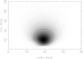
(a) (b)

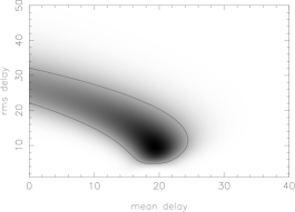
(c) (d)

Figure 4: Top, acausal (left) and causal (right) $\chi^{2}$ surfaces for Gaussian transfer function fitting to the HST lightcurve 3. Bottom, best-fit (solid line) and trial (dashed line) time-delay transfer functions to HST Exp. 6. The response is $\psi(\tau)$.

The Gaussian model investigated above is acausal because it permits HST response preceding the X-ray driving. We can construct a causal model by truncating the negative delay tail of the Gaussian. Panels (c) and (d) of Fig. 4 illustrate the results for the causal Gaussian fits in the same format as panels (a) and (b) of the same figure. The best fit for the causal Gaussian fitting has $\chi^{2}_{min}/779=1.230$. The parameters $\tau_{0}$ and $\Delta\tau$ become anti-correlated because the data to first order constrain the first and second moments of the delay distribution.

Table 1: Summary of results from parameterised Gaussian fitting to HST lightcurves. The rows give respectively the photometric phase, number of data points, reduced $\chi^{2}$, mean delay, RMS delay and integrated response for each light curve. Uncertainties are based on 1-parameter, 1-sigma confidence regions. The integrated response, $\Psi$, has been normalised by dividing by the mean of each HST light curve.

	Exp. 4	Exp. 5	Exp. 6	Exp. 7
$\phi_{\rm phot}$	0.36	0.39	0.42	0.44
N	528	541	782	704
$\chi^{2}_{min}/(N-3)$	1.193	1.446	1.230	1.159
$\tau_{0}$ (s)	$8.3\pm 4.0$	$16.0^{+2.5}_{-2.2}$	$19.3\pm 2.2$	$13.3^{+4.7}_{-4.5}$
$\Delta\,\tau$ (s)	$20.0^{+6.8}_{-7.0}$	$8.6^{+2.7}_{-2.3}$	$10.8^{+3.7}_{-3.3}$	$13.5^{+7.7}_{-4.7}$
$\Psi/10^{-3}$	$29\pm 1$	$32\pm 2$	$55^{+11}_{-7}$	$49\pm 5$

Table 1 summarises the results of fitting Gaussian transfer functions to the 4 data segments. For all 4 data segments the mean and RMS delays are roughly consistent within the 1-parameter 1-sigma uncertainties. A weighted average yields $\overline{\tau_{0}}=14.6\pm 1.4$ s, $\overline{\Delta\tau}=10.5\pm 1.9$ s. The total response, $\Psi$, is normalised using the mean count rate for the individual light curve. This normalised total response appears to be roughly constant for the two lightcurves from PRISM/RD, at a value of $\Psi\sim 30\times 10^{-3}$ and for the two lightcurves from PRISM/BL, at a value of $\Psi\sim 50\times 10^{-3}$. This difference between the values of $\Psi$ shows that the variability is stronger at short wavelengths, and suggests that the reprocessing therefore occurs in a relatively hot part of the system.

5 Discussion

It is clear from our analysis that reprocessing with a mean time delay of under 25 s dominates. This is the size of lag to be expected from the accretion disc assuming established system parameters (Orosz & Bailyn 1997, van der Hooft et al. 1998). Together with the narrowness of the transfer function (RMS delay $\sim~{}10$ s), this means that disc reprocessing must dominate over the secondary star, from which lags of greater than 40 s are expected at this binary phase ($\phi~{}\sim~{}0.40$). Even allowing for the maximum uncertainty in system parameters estimated by van der Hooft et al. [1998], our results are definitely inconsistent with the dominant source of reprocessing being the companion star. The response for the Gaussian fits, when normalised to the count rate for the light curves are consistent for the two PRISM/BL light curves and for the two PRISM/RD ones. The higher response, and hence reprocessing fraction, for the PRISM/BL agrees with this analysis of the mean and RMS delays, showing that the accretion disc is the most important region for reprocessing of X-rays in GRO J1655–40.

Why is this the case? During the activity observed by van der Hooft et al. [1997], light curve analysis revealed that X-ray heating of the companion star was important; if that was the case here, we should see echoes originating from the companion star. One explanation for why we do not is that the X-ray absorbing material in the disc may have a significant scale height above the mid-plane so that the companion would effectively be shielded from direct X-ray illumination, thus reducing the strength of reprocessing. For this to be the case, then the shielding material must rise to $H/R\sim 0.25$.

If the accretion disc in GRO J1655–40 is significantly irradiated, we now must ask why the long term optical light curve appears almost anticorrelated with X-ray behaviour? One possibility is that the irradiating X-ray flux is being increasingly attenuated by a disc corona. As the optical depth of the Compton scattering corona increases, we might naturally expect two consequences: firstly the hard X-rays, believed to be produced by Comptonisation, would increase. Secondly, the irradiation of the outer disc would decrease, as X-rays moving nearly parallel to the disc must penetrate a large optical depth of scattering material. We would thus expect that the optical/UV and hard X-ray light curves might appear anticorrelated, exactly as observed. Indeed, a related scenario was proposed by Mineshige [1994] to explain why the onset of an optical reflare in X-ray Nova Muscae 1991 occured simultaneous to a decrease in the Thomson optical depth deduced from X-ray spectra.

These observations represent a step forward in our understanding of SXTs. This is the first time that correlated optical–X-ray variability has been detected from a transient source and supports the picture, often assumed, that SXTs in outburst have irradiated accretion discs similar to those in persistent LMXBs.

References

- [1997] Christensen J. A., Welsh W. F., Evans I. N., Reinhart M., Hayes J. J. E., 1997, CAL/FOS ISR 150, STScI
- [1988] Edelson R. A., Krolik J. H., 1988, ApJ, 333, 646
- [1987] Gaskell C. M., Peterson B. M., 1987, ApJS, 65, 1
- [1995] Harmon B. A., et al., 1995, Nat, 374, 703
- [1998] Hynes R. I., et al., 1998, MNRAS, accepted
- [1980] Ilovaisky S. A., Chevalier C., White N. E., Mason K. O. Sanford P. W., Delvaille J. P., Schnopper H. W., 1980, MNRAS, 191, 81
- [1995] Keyes C. D., Koratkar A. P., Dahlem M., Hayes J., Christensen J., Martin S., 1995, Faint Object Spectrograph Instrument Handbook, 6th Edn. STScI, p. 52
- [1998] King A. R., Ritter H., 1998, MNRAS, 293, L42
- [1976] Middleditch J., Nelson J. E., 1976, ApJ, 208, 567
- [1994] Mineshige S., 1994, ApJ, 431, L99
- [1997] Orosz J. A., Bailyn C. D., 1997, ApJ, 477, 876
- [1993] Peterson B. M., 1993, PASP, 105, 247
- [1981] Petro L. D., Bradt H. V., Kelley R. L., Horne K., Gomer R., 1981, ApJ, 251, L7
- [1996] Remillard R., Bradt H., Cui W., Levine A., Morgan E., Shirey B., Smith D., 1996, IAU Circ. 6393
- [1996] Tanaka Y., Shibazaki N., 1996, ARA&A, 34, 607
- [1997] van der Hooft F. et al., 1997, MNRAS, 286, L43
- [1998] van der Hooft F., Heemskerk M. H. M., Alberts F., van Paradijs J., 1998, A&A, 329, 538
- [1994] White R. J., Peterson B. M., 1994, PASP, 106, 879