A VLA STUDY OF 15 3CR RADIO GALAXIES

Abstract

We present VLA radio maps in total intensity and polarization at 1.4, 4.9 and 8.4 GHz of fifteen 3CR radio galaxies for which good maps showing the large-scale radio structure have not previously been available. Previously unknown cores are detected in several sources and a bright one-sided jet in 3C 287.1 is mapped for the first time; several other jet-like features are also imaged. Total and core fluxes are tabulated and radio core positions are listed and compared to optical positions. The galaxy at the optical position listed for 3C 169.1 is found to lie farther from the radio core position than another dimmer, bluer galaxy. We discuss individual sources in some detail.

1 INTRODUCTION

This paper is the first in a series dealing with a comparison of the optical and radio properties of a sample of 3CR radio galaxies with $0.15<z<0.65$. The sample was taken from the Revised 3C Catalog of Radio Sources of Smith, Spinrad & Smith (1976) as updated by Spinrad et al. (1985) and Spinrad et al. (1991). In total, there are 66 objects in the sample and good quality radio maps showing the large-scale radio structure were found in the literature for 51 of these objects. We observed the remaining 15 objects with the VLA. In future papers, results of the radio-optical comparison will be presented. Here we discuss the new VLA images that were obtained.

Listed in Table 1 are the observed sources along with their optical positions, redshifts, 178 MHz flux densities on the scale of Baars et al. (1977), and spectral indices between 178 and 750 MHz. (The spectral index $\alpha$ is defined throughout in the sense $S\propto\nu^{-\alpha}$.) The optical positions and redshifts are taken from Spinrad et al. (1991). The 178 MHz flux densities are from Kellermann, Pauliny-Toth & Williams (1969) except for 3C 268.2 and 3C 306.1 which are taken from Pilkington & Scott (1965) and Gower, Scott & Wills (1967) (both taken from NED (1997)), respectively, because their values in Kellermann et al. (1969) are likely contaminated with confusing flux. All fluxes were adjusted to the scale of Baars et al. (1977) using the corrections given in Laing & Peacock (1980). The spectral indices are also consistent with the scale of Baars et al. (1977). They were taken from Laing, Riley & Longair (1983) if available (3C 16, 3C 220.1, 3C 401), or computed using the 178 MHz flux densities given here and 750 MHz flux densities from Kellermann et al. (1969) adjusted to the scale of Baars et al. (1977) using the corrections given in Laing & Peacock (1980). Also included in Table 1 are the rest frame luminosity at 178 MHz, the scale, the largest angular size (measured from the best available maps), and the linear size of the source. A Friedmann cosmology with H₀ = 50 km s^-1 Mpc^-1 and q₀ = 0 was used in the calculation of these quantities and is assumed throughout this paper.

Table 2 contains the position of the radio core for each source, the frequency of the map used to determine the core position, the reference for the core position, other radio map references, the optical spectral type of the object (i.e. the “optical class”) and the reference for this type. The optical type was taken directly from Jackson & Rawlings (1997) who use slightly different notation than that used here. Their “quasar/weak quasar” (Q/WQ) classification is equivalent to our broad-line (B) type. Similarly, their “high-excitation galaxy” (HEG) corresponds to our narrow line (N) type and their “low-excitation galaxy” (LEG) is our low-excitation (E) type. The references for the optical spectra on which these classifications are based can be found in Jackson & Rawlings (1997). References giving additional spectral information that are not found in Jackson & Rawlings (1997) are included in the Optical Reference column.

2 THE OBSERVATIONS

The data presented in this paper are from six separate sets of observations which are summarized in Table 3. Most observations were made at L-band in order to map the steep-spectrum extended structure of the sources. The C- and X-band observations aid in the detection and study of the flatter spectrum cores, jets and hot spots. All observations were made at two observing frequencies which were later averaged to give a map at a single effective frequency. At L-band these were 1.365 and 1.435 GHz, at C-band these were 4.835 and 4.885 GHz, and at X-band they were 8.415 and 8.465 GHz. A bandwidth of 50 MHz was used for all observations.

All data were reduced using the AIPS software package in the standard manner. 3C 48 and 3C 286 were used as primary flux and polarization position angle calibrators. Bad scans were removed from the calibrator data until acceptable amplitude and phase solutions were obtained using nearby point sources as phase calibrators. These solutions were then applied to the program sources. For the L-band data, a small first-order correction for ionospheric Faraday rotation (corresponding to at most a few degrees at the frequencies used) was applied using the AIPS task farad. This correction was based on mean monthly sunspot data as ionospheric measurements were not available. Finally, a series of self-calibrations was performed to further improve the maps. Typically we applied 2 to 3 phase-only self-calibrations followed by 1 to 2 phase and amplitude self-calibrations. The self-calibration procedure was stopped when no significant improvement in the map was seen.

3 THE MAPS

Most maps were made using the AIPS task imagr, with robustness between zero and one (intermediate between uniform and natural weighting) to improve the noise properties of the maps. For a very few sources the flux difference between the two observing frequencies contributed significantly to the off-source noise at 1.4-GHz; in these cases the two frequencies were mapped separately, a spectral index was determined, and the visibility amplitudes were corrected to the average frequency with imagr before mapping. The 4.86-GHz map of 3C 357 was made with AIPS task apcln. The 4.86-GHz map of 3C 456 was made with AIPS task mx. Both 4.86-GHz maps were provided courtesy of J. Stocke.

Polarization maps as well as total intensity maps are presented for most sources. However, we have no polarization information for the objects observed at 1.4-GHz in the A-configuration or for the 4.86-GHz observations because no suitable polarization calibration data were available. Polarization vectors are only plotted where both the total and polarized intensities exceed three times the appropriate r.m.s. noise. The lengths of the vectors on the polarization maps indicate the degree of polarization; their directions indicate the directions of the electric field. If the Faraday rotation measure (RM) along the line of sight is sufficiently low, lines perpendicular to these vectors would be parallel to the emission-weighted mean projected direction of the magnetic field vector in the radio source. The integrated rotation measures towards these sources, where known, are low (Simard-Normandin, Kronberg & Button 1981); however, the rotation measures towards particular regions of the sources are not known, and so the vector directions must be interpreted with caution.

For two sources, maps of spectral index between 1.4 and 8.44-GHz are presented. These were made with matching longest and shortest baselines, and appropriate weighting, to minimize systematic errors induced by different uv coverages. Only regions where the signal exceeded three times the r.m.s. noise on both maps are plotted.

Information concerning the maps presented here is summarized in Table 4. The dynamic ranges listed in the second to last column are defined as the peak map flux divided by the r.m.s. noise in the map; the noise approaches the expected thermal value in many cases in total-intensity maps and in almost all maps in Stokes Q and U. The beam size in the last column is the FWHM along the major and minor axes of the restoring elliptical Gaussian, obtained by fitting to the dirty beam. This beam is shown in one of the corners of each map. The contour levels and the location of the peak flux are given in the figure captions.

4 POLARIZATION

Since 3C 348 was observed at two different epochs, a check on the systematic difference of the 1.4-GHz polarization maps is possible. A comparison of the position angles of the polarization maps made at these two different epochs shows the systematic difference (reflecting systematics in, among other things, the polarization angle calibration and the correction for ionospheric Faraday rotation) to be $<$ 1^∘. The r.m.s. is of the order of a few degrees, which is about what we expect. Thus the polarization calibration appears to have worked well.

5 FLUXES AND POSITIONS

Total fluxes are given in column 4 of Table 5. In general, the error in the total flux is $\simeq$ 5%. This includes both the calibration error and the on-source error. Column 3 of Table 5 lists the ratio of the largest angular size of the source to the largest scale structure visible to the VLA configuration and frequency with which the source was observed. If this ratio is $\gtrapprox$ 1 then the source may be undersampled; that is, large scale structure (i.e. structure with angular size $\gtrapprox$ $\theta_{MAX}$) will be missing from the map and the total flux presented in Table 5 will be lower than the true value. Fluxes from individual structures smaller than $\theta_{MAX}$, such as point sources, are not affected by this undersampling. A ratio $>$ 1 does not necessarily mean that the source is undersampled, however. For example, a source could be composed of several components that are all visible to the array but the combined angular size of all these components is larger than the largest scale structure visible to the array. In this case, no structure or flux would be missing from the map. For this work, the severity of the undersampling is determined by comparing the total fluxes from our maps with single-dish total fluxes from the literature (listed in column 7) and with fully sampled maps at the same frequency, if available. Total fluxes in Table 5 marked with a dagger indicate probable undersampling and are discussed in the comments on individual sources. Either these fluxes are too low to agree (within the errors) with the values in the literature or, in the case of the 8.44-GHz fluxes, LAS/$\theta_{MAX}$ $>$ 1 and no reliable comparison fluxes are available. Single-dish fluxes from the literature are presented in column 7. If published values agreed, an average value with an appropriate error is listed. (If no error was given in the literature, a value of 5% was assumed.) If published values were not in agreement, a range of values is listed. This disagreement may be an indication of source variability. Wright & Otrupcek (1990) provided an 8.4-GHz comparison flux for 3C 63 although no error was given. Other 8.4-GHz comparison fluxes were estimated using $\alpha^{5000}_{750}$ and $\sim$5-GHz fluxes. The $\alpha^{5000}_{750}$ values used were those of Kellermann et al. (1969) adjusted to the flux scale of Baars et al. (1977) using the corrections given in Laing & Peacock (1980).

Core flux densities or upper limits are given in column 5 of Table 5. These flux values were determined by one of four methods. If the core was visible and relatively isolated, a point source with characteristics matching those of the beam given in Table 4 was fit to the core using the AIPS task imfit. The integrated flux from this point-source fit is taken to be the core flux. If the core was visible but surrounded by confusing flux, a two-component fit using a point source and an additional sloping background was performed and the integrated flux from the point-source fit is quoted in Table 5. If the core was not visible, the lobes of the source were removed by subtracting Gaussian fits, again using imfit. If the core then became apparent at the appropriate position (a previously identified radio core position or the optical position if no core position was available), imfit was used to fit a Gaussian point source to it as above. Core fluxes obtained in this manner are marked with an asterisk and an estimate of the uncertainty of these core fluxes is given below. If the core still was not visible, a value of 3 $\times$ the on-source r.m.s. is listed as an upper limit for the core flux.

The error for the core flux given in column 6 of Table 5 is the value returned by imfit. This is the flux error due to the uncertainty of the fit only and does not include the $\sim 5$% calibration and on-source error. For most cases, the error returned by imfit is much larger than 5% and so this additional error may be neglected. However, when the error from imfit is $<$ 10% of the core flux (3C 63, 3C 277, 3C 287.1, 3C 357 and 3C 456), the additional 5% error should be included to obtain a more realistic value.

To estimate the uncertainty of core fluxes measured from lobe-subtracted maps, the procedure was performed on a 4.86-GHz B-configuration map of 3C 456 from Stocke (1994). (This map is not presented in this paper because the structure is nearly identical to that in the 1.4-GHz map presented here.) When compared to the core flux from the A-configuration map of the same frequency given in Table 5, the core flux obtained from the lobe-subtracted map was low by 30%. This gives a rough estimate of the uncertainty of the fluxes determined by this method and indicates that the error returned by imfit may be a substantial underestimate of the true error in these cases. However, this source is more complicated and required the removal of 3 components (see discussion in section 6.14) rather than 2 components like the other sources (3C 320, 3C 434 and 3C 459) and so this uncertainty may be an overestimate for these other sources. The position of the core obtained from the lobe-subtracted map was only 0.22^′′ different from that obtained from the point source fit to the A-configuration map. This indicates that the structure remaining after the lobes were subtracted was indeed the core.

Radio core positions, taken either from our maps or from the literature, are given in Table 2. Those marked with an asterisk denote probable cores detected only after the removal of the radio lobes. No radio core position is given for 3C 16 since no core detection is known. Core positions taken from maps presented in this paper typically have errors of 0.35^′′ in each direction. An examination of the optical positions in Table 1 shows that they are within 1^′′ of the radio core positions for most sources. Since errors in the optical position are assumed to be a minimum of 1^′′ in each direction, positions within 1^′′ of each other are in agreement. Differences between radio core and optical positions that are $>$ 1^′′ are discussed in the comments on individual sources. Comparisons of different radio core positions for the same source (i.e. core positions at different frequencies, core positions from different fits, core positions from the literature) are also discussed.

6 COMMENTS ON INDIVIDUAL SOURCES

6.1 3C 16

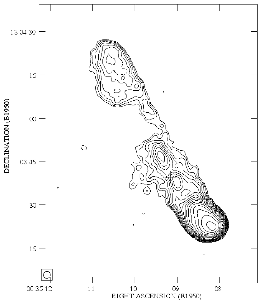
Figure 1: Left: Total intensity map of 3C 16 at 8.44 GHz. The contour levels are $0.1\times(-\sqrt{2},-1,1,\sqrt{2},2,2\sqrt{2},\dots)$ mJy beam^-1. Right: Polarization map. The contour levels are $0.1\times(-2,-1,1,2,4,\dots)$ mJy beam^-1. A vector of length one arcsecond corresponds to 20% polarization. A cross marks the position of the optical identification. The peak flux occurs in the southern lobe.

(Fig. 1). This source may be undersampled, though the total 8-GHz flux density is consistent with values predicted from the spectral index and 5-GHz fluxes. No point-like core is detected in our 8.44-GHz map and no core detections were found in the literature. Two extended knots of emission bracket the position of the optical identification, which lies on the NE edge of the southern knot. Due to the proximity of the optical position to this knot, the upper limit for the core flux given in Table 5 is a point source fit to this southern knot, rather than 3 $\times$ the on-source r.m.s. like the upper limits for the other non-detections. Neither of these knots is a likely core candidate due to their extended nature and their steep 1.4–8.4 GHz spectrum ($\alpha\sim 1$). The two knots may be pieces of an inner twin jet structure, but their steep spectrum and the fact that they were transversely resolved by Leahy & Perley (1991) make this unlikely as well. An alternative possibility is that they constitute lobes of a restarting radio source.

6.2 3C 63

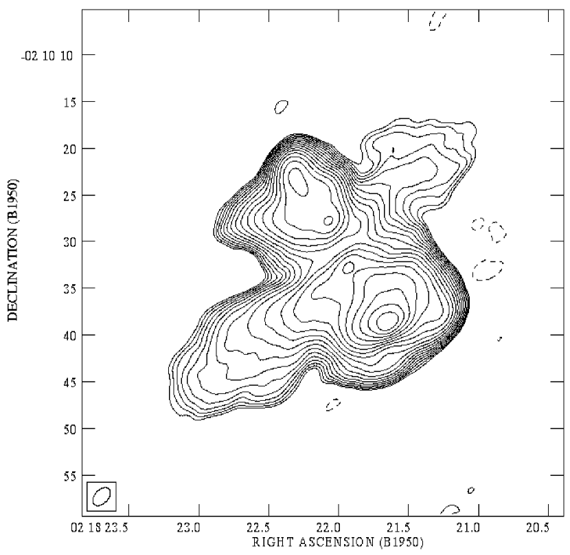
Figure 2: Total intensity map of 3C 63 at 1.4 GHz. The contour levels are $0.5\times(-\sqrt{2},-1,1,\sqrt{2},2,2\sqrt{2},\dots)$ mJy beam^-1. The peak flux occurs in the southern lobe.

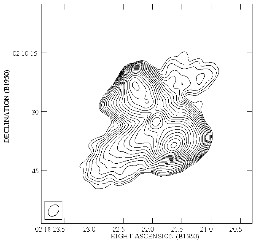
Figure 3: Left: Total intensity map of 3C 63 at 8.44 GHz. The contour levels are $0.1\times(-\sqrt{2},-1,1,\sqrt{2},2,2\sqrt{2},\dots)$ mJy beam^-1. Right: Polarization map. The contour levels are $0.1\times(-2,-1,1,2,4,\dots)$ mJy beam^-1. A vector of length one arcsecond corresponds to 20% polarization. The peak flux occurs in the southern lobe.

(Figs. 2-4). This source is probably undersampled at 1.4-GHz, and the total flux density is lower than some found in the literature. The 8.44-GHz map is well sampled and the total flux agrees (within the errors) with the value given in Wright & Otrupcek (1990). The similar core fluxes at 1.4 and 8.44-GHz indicate a flat or slightly inverted spectrum that is typical of a radio core. The core positions from our two maps agree to within 0.5^′′.

This source was previously observed by Baum et al. (1988) but the faint emission regions transverse to the radio axis, particularly the western region, are more prominent in both our maps. These regions constitute a new example of ‘wings’ (cf. Leahy & Perley 1991). They are strongly polarized (mean fractional polarization of $\sim$ 50% at X-band) and the apparent magnetic field is directed along the wings, transverse to the radio axis, as is typical in such features. The spectral index map also shows some interesting structure. The hotspots and core have the flattest spectra as expected, but the steep spectrum of the material around the hot spots at the sides of the source, particularly in the southern lobe, is unusual, since aged material is usually found only in the parts of the lobe nearest the core. This, together with the wings, suggests that the backflow velocities are very significant compared to hotspot advance speeds in this source.

6.3 3C 169.1

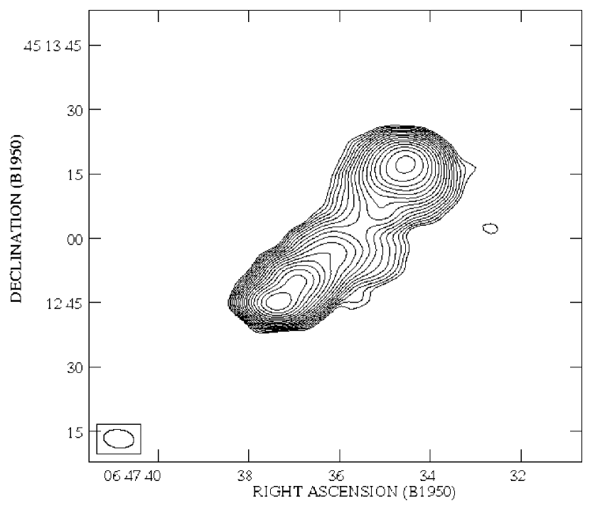
Figure 5: Left: Total intensity map of 3C 169.1 at 1.4 GHz. The contour levels are $0.8\times(-\sqrt{2},-1,1,\sqrt{2},2,2\sqrt{2},\dots)$ mJy beam^-1. Right: Polarization map. The contour levels are $0.8\times(-2,-1,1,2,4,\dots)$ mJy beam^-1. A vector of length one arcsecond corresponds to 10% polarization. The peak flux occurs in the southern lobe.

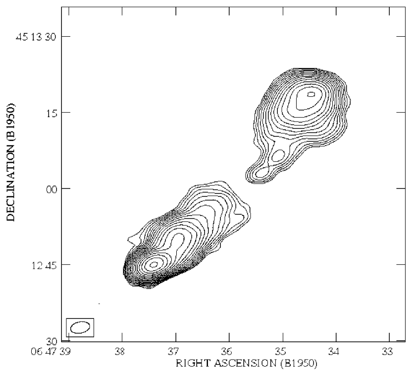
Figure 6: Left: Total intensity map of 3C 169.1 at 8.44 GHz. The contour levels are $0.15\times(-\sqrt{2},-1,1,\sqrt{2},2,2\sqrt{2},\dots)$ mJy beam^-1. Right: Polarization map. The contour levels are $0.15\times(-2,-1,1,2,4,\dots)$ mJy beam^-1. A vector of length one arcsecond corresponds to 20% polarization. The peak flux occurs in the southern lobe.

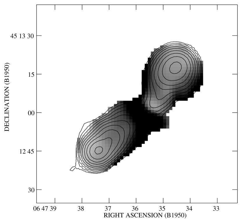
Figure 7: A 1.4-8.44 GHz spectral index map of 3C 169.1 (resolution $5.40\times 5.40$ arcsec). Spectral index values are given by the greyscale image and range from 0.5 (white) to 1.8 (black). Superposed are contours of the 8.44-GHz map at this resolution. The contour levels are $0.1\times(-2,-1,1,2,4,\dots)$ mJy beam^-1.

(Figs. 5-7). This source is probably undersampled at 8.44-GHz and the total flux density is somewhat lower than the values predicted from the spectral index and 5-GHz fluxes. The 1.4-GHz observation is well sampled and our total flux agrees with published values.

An unresolved radio core is detected in the 8.44-GHz map. This core position lies 2.5^′′ NW of the optical position given in Table 1. The errors in this core position are 0.5^′′ in R.A. and 0.2^′′ in Dec. and the errors in the optical position are given in Kristian, Sandage & Katem (1978) as $\sim$ 1^′′ in each direction. The combined errors are not large enough to account for the difference in the two positions. This is probably due to an underestimate of the optical position errors. However, our optical images show another galaxy closer to the radio core position. Preliminary measurements from these images show it to be within 1^′′. The position for this second galaxy given in Kristian et al. (1978) (although they refer to it as “starlike”) puts it 1.3^′′ from the radio core. This second galaxy is dimmer (m_r = 21.2 vs. 20.6) and bluer (g-r = 0.5 vs. 0.9) than the galaxy found at the optical position and, according to McCarthy et al. (1997), is blueshifted relative to the galaxy found at the optical position by 1000 km s^-1.

The 8.44-GHz map shows what appears to be a jet connecting the core to the northern lobe. The 1.4-GHz map shows a bulge of emission to the west, near the center of the source. The spectral index map shows the expected steepening back towards the core. The apparent jet in the northern lobe has a flatter spectrum than the material around it, which supports the idea that it actually is a jet rather than an extension of the lobe. A higher resolution L-band map which also shows evidence of the apparent jet can be found in Neff et al. (1995).

6.4 3C 220.1

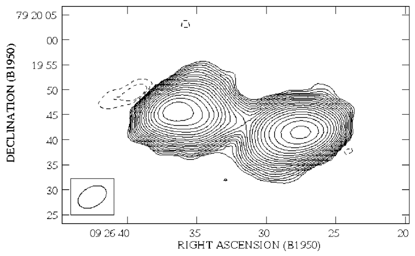
Figure 8: Left: Total intensity map of 3C 220.1 at 1.4 GHz. The contour levels are $1.0\times(-\sqrt{2},-1,1,\sqrt{2},2,2\sqrt{2},\dots)$ mJy beam^-1. Right: Polarization map. The contour levels are $1.0\times(-2,-1,1,2,4,\dots)$ mJy beam^-1. A vector of length one arcsecond corresponds to 1% polarization. The peak flux occurs in the western lobe.

(Fig. 8). The total flux in Table 5 agrees well with values found in the literature. The radio core position was measured from a higher resolution C-band map (Burns et al. 1984) and is accurate to 0.5^′′ in each direction. This core lies 1.9^′′ SE of the optical position listed in Table 1. The errors in the optical position are unknown but, assuming they are 1^′′ in each direction, the combined radio and optical positional errors account for the difference between the two positions. Optical images show no objects closer to the radio core. The 1.4-GHz map presented here shows no unusual features in this source. The degree of polarization at this frequency is unusually low (averaging $\sim 1$%); this may be evidence for intrinsic Faraday rotation from the X-ray halo found around 3C 220.1 by Hardcastle, Lawrence & Worrall (1998b).

6.5 3C 268.2

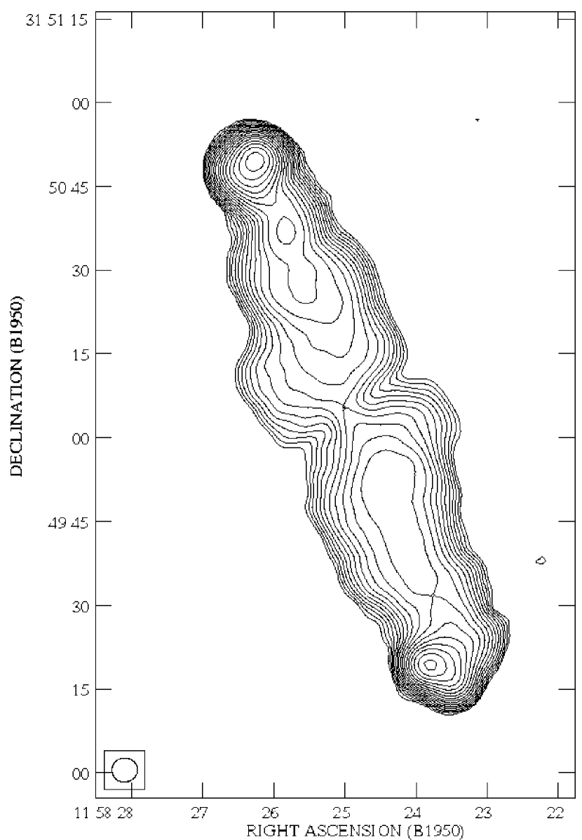
Figure 9: Left: Total intensity map of 3C 268.2 at 1.4 GHz. The contour levels are $0.4\times(-\sqrt{2},-1,1,\sqrt{2},2,2\sqrt{2},\dots)$ mJy beam^-1. Right: Polarization map. The contour levels are $0.4\times(-2,-1,1,2,4,\dots)$ mJy beam^-1. A vector of length one arcsecond corresponds to 20% polarization. The peak flux occurs in the northern lobe.

(Fig. 9). Although the LAS of this source is 0.94 $\times$ $\theta_{MAX}$ of the configuration used to observe it at 1.4-GHz, this source may be undersampled as flux densities in the literature are larger than the total flux density measured from our map. The radio core coordinates were taken from Strom et al. (1990) who measured them from a C-band WSRT map. This core lies 2.9^′′ NE of the optical position given in Table 1. No errors are given for the core coordinates in Strom et al. (1990) but the errors in the optical position are listed as 7^′′ in Wyndham (1966) and these are obviously sufficient to account for the positional difference. Measurements from optical images show no objects closer to the radio core and put the core in the host galaxy (although far from the center).

The lobes in the 1.4-GHz map presented here seem to curve away from the radio axis near the center of the source. This behavior is seen in a number of other sources (e.g. Leahy & Williams 1984). The heads of the lobes seem to have a “pinch” in the emission located about one-third of the distance from the leading edge back towards the center of the source. This effect is also observed in other radio galaxies such as 3C 349 (Hardcastle et al. 1997; Leahy & Perley 1991). A higher resolution L-band map in Neff et al. (1995) shows this pinching in the lobe shape more clearly, as well as some details of the hotspots.

6.6 3C 277

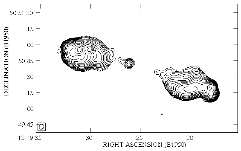
Figure 10: Left: Total intensity map of 3C 277 at 1.4 GHz. The contour levels are $0.3\times(-\sqrt{2},-1,1,\sqrt{2},2,2\sqrt{2},\dots)$ mJy beam^-1. Right: Polarization map. The contour levels are $0.3\times(-2,-1,1,2,4,\dots)$ mJy beam^-1. A vector of length one arcsecond corresponds to 20% polarization. The peak flux occurs in the eastern lobe.

(Fig. 10). Although our map of this giant source may be undersampled, the total flux density measured from our map is consistent with others in the literature. The core and a probable jet in the eastern lobe are visible in our 1.4-GHz map. Both lobes appear to have double hot spots.

6.7 3C 287.1

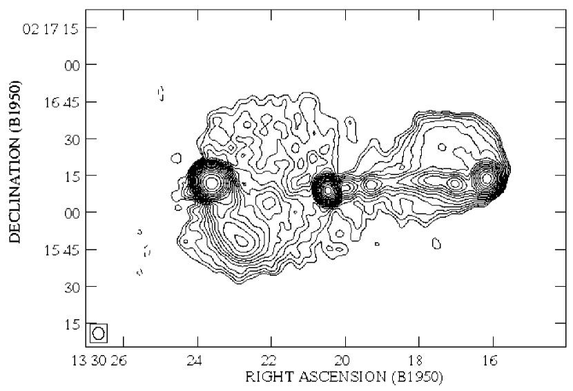
Figure 11: Left: Total intensity map of 3C 287.1 at 1.4 GHz. The contour levels are $0.7\times(-\sqrt{2},-1,1,\sqrt{2},2,2\sqrt{2},\dots)$ mJy beam^-1. Right: Polarization map. The contour levels are $0.7\times(-2,-1,1,2,4,\dots)$ mJy beam^-1. A vector of length one arcsecond corresponds to 20% polarization. The peak flux occurs in the hotspot in the eastern lobe.

(Fig. 11). The radio map of this broad-line radio galaxy is almost certainly undersampled, and the flux density measured from our map is lower than those found elsewhere. The core flux for this object is quite large and is a substantial portion (13%) of the total flux.

The core and a bright, knotty and slightly curved jet in the western lobe are clearly visible in the 1.4-GHz map. C-band maps can be found in Antonucci (1985) and Downes et al. (1986) but ours is the first map to show details of the jet. The low axial ratio (length to width) of the source, the prominent core, the one-sided nature of the jet and the broad-line spectrum (e.g. Eracleous & Halpern 1994) are all consistent with the object being aligned close to the line of sight. Hardcastle et al. (1998a) suggest that low-power broad-line radio galaxies of this sort are a low-redshift equivalent of the high-redshift lobe-dominated quasars, and the radio structure of this object is certainly consistent with that picture. If the jet’s one-sidedness is caused by relativistic beaming alone, then the jet-counterjet ratio of $\sim 6$ in the inner 30^′′, corresponding to the straight part of the jet, implies an angle to the line of sight of $<70^{\circ}$ and beaming velocities $>0.3c$.

6.8 3C 306.1

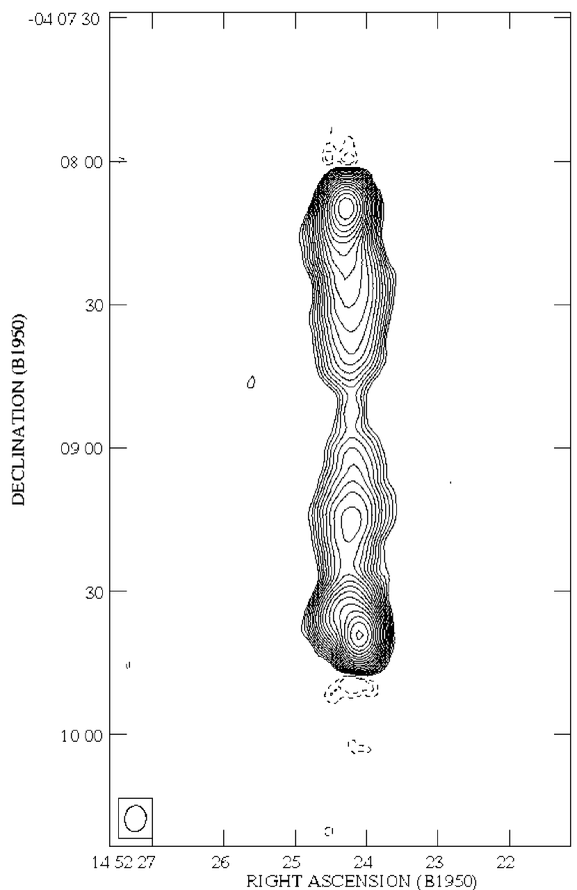
Figure 12: Left: Total intensity map of 3C 306.1 at 1.4 GHz. The contour levels are $1.0\times(-\sqrt{2},-1,1,\sqrt{2},2,2\sqrt{2},\dots)$ mJy beam^-1. Right: Polarization map. The contour levels are $1.0\times(-2,-1,1,2,4,\dots)$ mJy beam^-1. A vector of length one arcsecond corresponds to 20% polarization. The peak flux occurs in the southern lobe.

(Fig. 12). This source is not likely to be undersampled. An unresolved radio core is detected in the 1.4-GHz map. This core position lies 4.2^′′ W and 5.8^′′ S of the optical position listed in Table 1. Although the errors of the optical position are given as 7^′′ by Wyndham (1966), we checked the optical identification by examining images corresponding to the radio core position in the Digitized Sky Survey (STScI 1997). This procedure returned the same galaxy as that marked on the finding chart of Wyndham (1966) with coordinates matching those of the radio core to within 0.4^′′. Thus, the optical position does indeed coincide with the radio core. Our 1.4-GHz map may show some pinching of the southern lobe (and perhaps the northern lobe to a lesser extent), but otherwise there is very little distortion in the radio structure.

6.9 3C 320

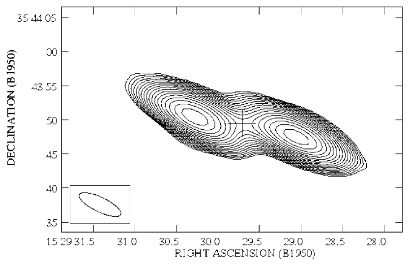
Figure 13: Left: Total intensity map of 3C 320 at 8.44 GHz. The contour levels are $0.1\times(-\sqrt{2},-1,1,\sqrt{2},2,2\sqrt{2},\dots)$ mJy beam^-1. Right: Polarization map. The contour levels are $0.1\times(-2,-1,1,2,4,\dots)$ mJy beam^-1. A vector of length one arcsecond corresponds to 5% polarization. A cross marks the position of the probable core discussed in the text. The peak flux occurs in the eastern lobe.

(Fig. 13). This source is not undersampled. A radio core is not apparent in our map; however, when the two lobes are removed, a structure resembling a core remains. A point source fit to this structure yields the core flux in Table 5 and the core position in Table 2. The core is located almost exactly halfway between the peaks of the two lobes and lies only 1.0^′′ from the optical position given in Table 1.

6.10 3C 348

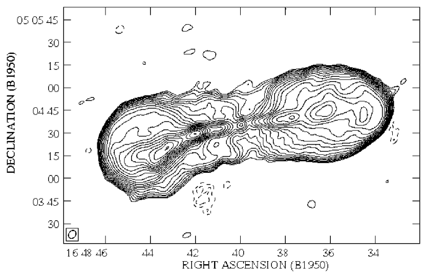
Figure 14: Left: Total intensity map of 3C 348 at 1.4 GHz. The contour levels are $2.0\times(-\sqrt{2},-1,1,\sqrt{2},2,2\sqrt{2},\dots)$ mJy beam^-1. Right: Polarization map. The contour levels are $2.0\times(-2,-1,1,2,4,\dots)$ mJy beam^-1. A vector of length one arcsecond corresponds to 10% polarization. The peak flux occurs in the jet in the eastern lobe.

(Fig. 14). Also known as Hercules A, this source has one of the highest measured low-frequency radio flux densities. We observed this source at two different epochs. Although LAS/$\theta_{MAX}$ indicates this source might be affected by undersampling, the total fluxes in Table 5 agree well with published values and there does not seem to be much evidence for missing flux. This may be a case where the sum of the angular sizes of all the components making up the source is larger than $\theta_{MAX}$ but all the individual components are still seen by the array. Our two fluxes also agree with each other (within the errors), as do our two core fluxes; the data from the two epochs are therefore combined in the map presented here. The core positions from the two different observations agree to within 0.04^′′.

This source was previously observed at C-band by Dreher & Feigelson (1984) who remarked on its peculiar jet-dominated morphology for a source of such high radio power. Our 1.4-GHz map shows a weak core as well as the strong jets. The extended emission is very symmetric about the radio axis. Polarization maps show a strong asymmetry in fractional polarization, with the western lobe being much less strongly polarized than the eastern one. The fact that the more prominent eastern jet lies in the more strongly polarized lobe combined with the fact that the source lies in a cluster with strong X-ray emission has led Gizani & Leahy (1996, and in prep.) to treat it as an example of the Laing-Garrington effect (Laing 1988; Garrington et al. 1988).

6.11 3C 357

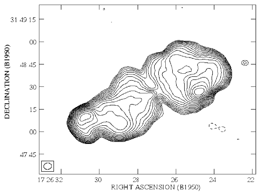
Figure 15: Left: Total intensity map of 3C 357 at 1.4 GHz. The contour levels are $0.5\times(-\sqrt{2},-1,1,\sqrt{2},2,2\sqrt{2},\dots)$ mJy beam^-1. Right: Polarization map. The contour levels are $0.5\times(-2,-1,1,2,4,\dots)$ mJy beam^-1. A vector of length one arcsecond corresponds to 20% polarization. The peak flux occurs in the western lobe.

(Figs. 15-16). This source is severely undersampled at 4.86-GHz, but there does not appear to be a problem at 1.4-GHz. The radio core lies 1.6^′′ NW of the optical position listed in Table 1. The optical position is accurate to 1^′′ in each direction according to Véron (1966) and the core position errors are 0.1^′′ in each direction. When combined, these positional errors account for nearly all the difference between the two positions. Measurements from an optical image put the radio core in the host galaxy (although not at the center). The positions and fluxes of the cores at 1.4 and 4.86-GHz are consistent.

The 4.86-GHz map shows multiple hot spots in both lobes. The core is also visible and a jet points toward the most compact hot spot in the NW lobe. The 1.4-GHz map shows some large-scale structure. The NW lobe is odd in that the pair of less compact hotspots is positioned very asymmetrically with respect to the lobe itself and the axial ratio of this lobe is close to unity. The SE lobe is extended to the N, suggesting non-axisymmetric backflow close to the center of the source.

6.12 3C 401

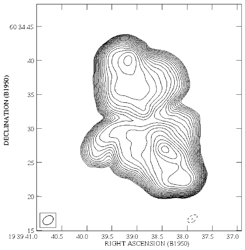
Figure 17: Total intensity map of 3C 401 at 1.4 GHz. The contour levels are $0.4\times(-\sqrt{2},-1,1,\sqrt{2},2,2\sqrt{2},\dots)$ mJy beam^-1. The peak flux occurs in the jet in the southern lobe.

(Fig. 17). This source is well sampled by our observations and our total flux density agrees with the values in the literature. The core position was measured from a higher resolution 8.44-GHz map in Hardcastle et al. (1997) and is accurate to better than 0.1^′′. The 1.4-GHz core position is within 1^′′ of this 8.44-GHz core position. A point source fit to the radio core seen in the L-band map of Leahy et al. (1997) gives an L-band core flux of 21 mJy, consistent with our measured value.

Our 1.4-GHz map shows both lobes extending away from the radio axis close to the central regions of the source. Emission from the bright one-sided jet is also visible in the southern lobe; this feature is more clearly seen in the maps of Hardcastle et al. (1997) and Leahy et al. (1997).

6.13 3C 434

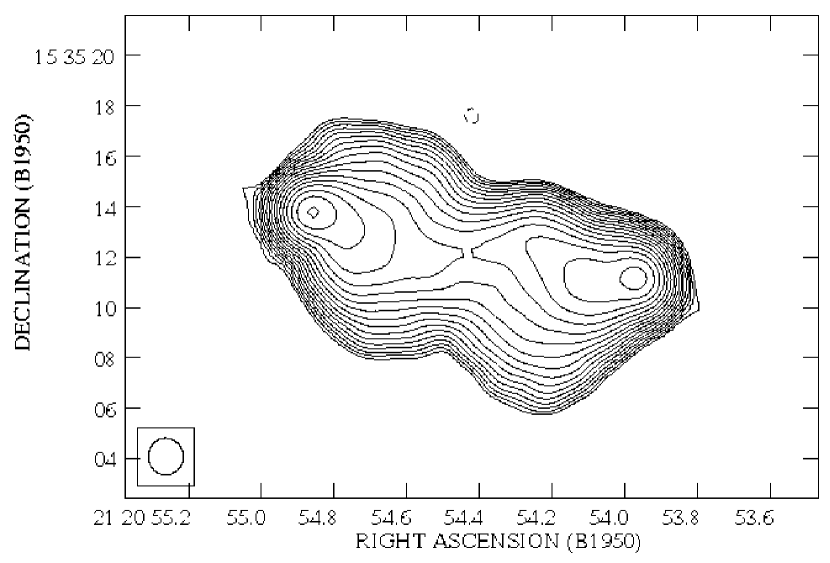
Figure 18: Total intensity map of 3C 434 at 1.4 GHz. The contour levels are $0.5\times(-\sqrt{2},-1,1,\sqrt{2},2,2\sqrt{2},\dots)$ mJy beam^-1. The peak flux occurs in the eastern lobe.

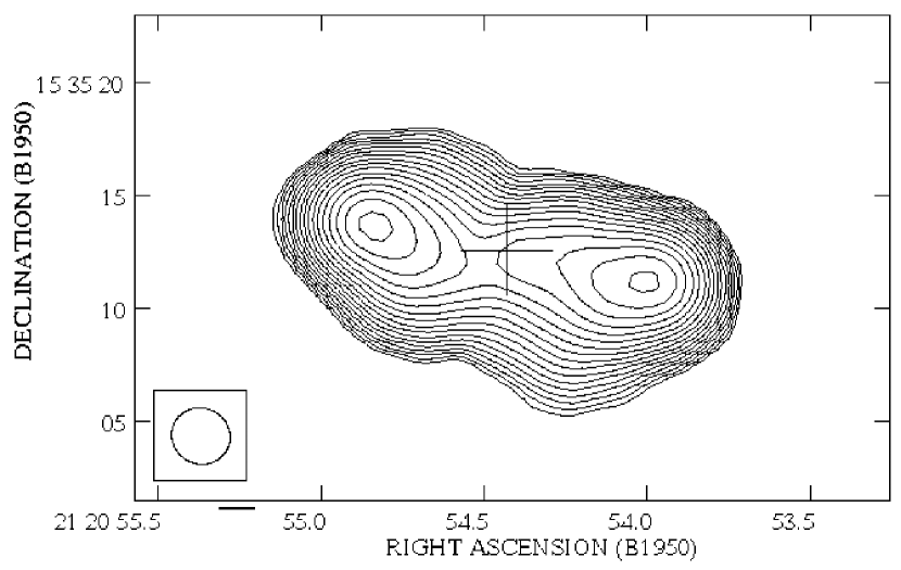
Figure 19: Left: Total intensity map of 3C 434 at 8.44 GHz. The contour levels are $0.2\times(-\sqrt{2},-1,1,\sqrt{2},2,2\sqrt{2},\dots)$ mJy beam^-1. Right: Polarization map. The contour levels are $0.2\times(-2,-1,1,2,4,\dots)$ mJy beam^-1. A vector of length one arcsecond corresponds to 20% polarization. A cross marks the position of the probable core discussed in the text. The peak flux occurs in the eastern lobe.

(Figs. 18-19). This source is not undersampled at either observing frequency and our 1.4-GHz total flux agrees with published values. A radio core is not apparent in either map. However, when the two lobes are removed from the 8.44-GHz map, a structure resembling a core remains. A point source fit to this structure yields the core flux in Table 5 and the core position in Table 2. The core is located almost exactly halfway between the peaks of the two lobes and lies only 1.0^′′ from the optical position given in Table 1. When the lobes are removed from the 1.4-GHz map, no core-like structure is seen. The broad lobes seen in the 1.4-GHz map are both slightly extended to the south near the center of the source.

6.14 3C 456

(Figs. 20-21). The A-configuration 4.86-GHz map presented in Fig. 21 is definitely undersampled. A B-configuration 4.86-GHz map of Stocke (1994) (LAS/$\theta_{MAX}$ = 0.34) shows large scale structure almost identical to that in the 1.4-GHz map shown in Fig. 20 and this structure is clearly missing from the map in Fig. 21. Due to this undersampling problem, the total 4.86-GHz flux in Table 5 is taken from the B-configuration map of Stocke (1994). This flux, which is 26% larger than the total flux measured from Fig. 21, agrees with values in the literature. The 1.4-GHz map is not undersampled and the total flux from this map agrees with published values.

The radio core position and 4.86-GHz core flux are taken from the map presented in Fig. 21. The radio core lies 1.3^′′ SW of the optical position listed in Table 1. The optical position is accurate to 1^′′ in each direction according to Véron (1966) and these errors account for the difference in the two positions (the errors in the core position are $<0.1^{\prime\prime}$). The core is not apparent in the 1.4-GHz map but when the lobes are removed (3 Gaussians were used to remove the lobes - see Fig. 21), a structure resembling a core remains. A point source fit to this structure yields the 1.4-GHz core flux in Table 5 and a core position within 0.2^′′ of that listed in Table 2. Removing 3 Gaussians from the B-configuration 4.86-GHz map of Stocke (1994) and fitting the remaining structure with a point source yields a core position within 0.3^′′ of that given in Table 2 but the core flux in this case is only 23 mJy, substantially smaller than that measured directly from Fig. 21.

The 1.4-GHz map shows a small, unusually asymmetrical source. The faint extension to the east and west of the bright northern lobe is probably a deconvolution artifact. The 4.86-GHz map shows a core with a strong northern lobe or hot spot with a probable bright backflow feature (the inner northern component) and a much weaker southern lobe or hot spot. A possible alternative interpretation is that the inner northern component is actually a foreground or background source. However, optical images show no evidence of another object near this position. The extension to the east of the northern lobe/hotspot in the 4.86-GHz map is probably a deconvolution artifact as well.

6.15 3C 459

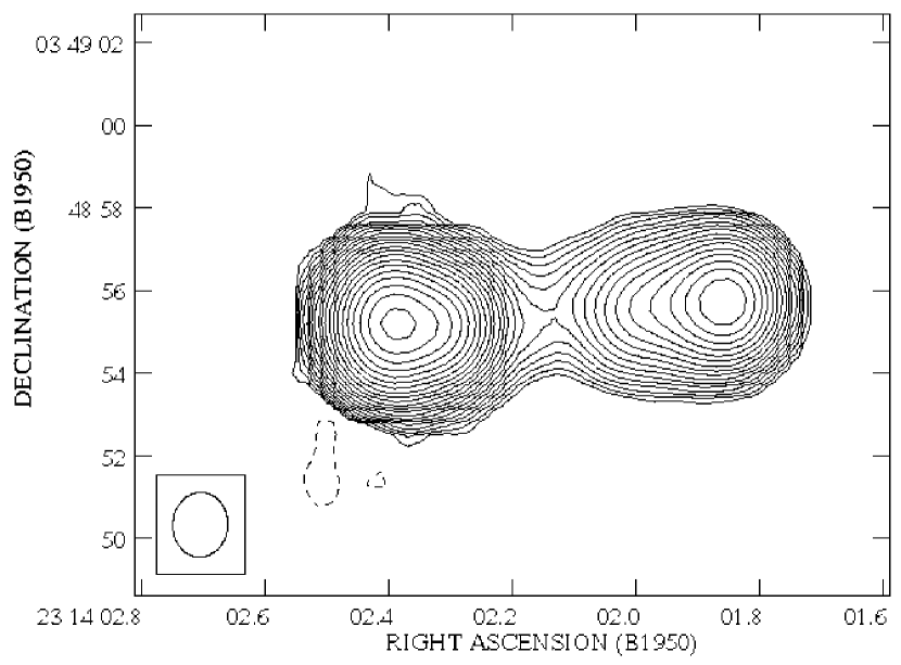
Figure 22: Total intensity map of 3C 459 at 1.4 GHz. The contour levels are $2.0\times(-\sqrt{2},-1,1,\sqrt{2},2,2\sqrt{2},\dots)$ mJy beam^-1. The peak flux occurs in the eastern lobe.

(Fig. 22). The total flux of this small steep-spectrum source agrees with values in the literature. The core is not apparent in this map. However, when the two lobes are removed, a structure resembling a core remains. A point source fit to this structure yields the core flux in Table 5. This flux is not consistent with the fluxes measured by Ulvestad (1985) if his suggestion that the core is steep-spectrum holds at these lower frequencies; however, the position of the core obtained from this fit lies less than 0.4^′′ from the core position of Ulvestad (1985) given in Table 2 which was taken from his high resolution U-band (2 cm) map. The C-band map of Morganti et al. (1993) appears to be contaminated by imaging artifacts.

Table 1: The Sample of Sources

Source	R.A.	Dec.	$z$	$S_{178}$	$\alpha^{750}_{178}$	$P_{178}$ (1024	Scale	LAS	Size
	(B1950.)	(B1950.)		(Jy)		W Hz-1 sr-1)	(kpc/′′)	(′′)	(kpc)
3C 16	00 35 09.16	+13 03 39.6	0.406	12.2	0.94	976	7.18	80.3	577
3C 63	02 18 21.90	$-$02 10 33.	0.175	20.9	0.82	252	4.01	50.0	200
3C 169.1	06 47 35.5	+45 13 01.	0.633	8.0	0.93	1830	9.08	64.0	581
3C 220.1	09 26 31.87	+79 19 45.4	0.620	17.2	0.93	3750	9.00	45.4	408
3C 268.2	11 58 24.8	+31 50 02.	0.362	7.5	0.79	441	6.70	112.7	755
3C 277	12 49 26.15	+50 50 42.9	0.414	8.2	0.92	680	7.26	159.2	1157
3C 287.1	13 30 20.46	+02 16 09.0	0.2159	8.9	0.55	160	4.70	139.9	658
3C 306.1	14 52 24.5	$-$04 08 47.	0.441	12.4	0.81	1150	7.53	108.0	814
3C 320	15 29 29.70	+35 43 48.5	0.342	9.9	0.78	510	6.46	37.0	239
3C 348	16 48 39.98	+05 04 35.0	0.154	382.6	1.03	3620	3.62	202.2	732
3C 357	17 26 27.41	+31 48 23.9	0.1664	10.6	0.60	111	3.85	118.0	454
3C 401	19 39 38.84	+60 34 32.6	0.201	22.8	0.71	362	4.46	26.4	118
3C 434	21 20 54.40	+15 35 11.7	0.322	5.2	0.64	226	6.22	21.6	134
3C 456	23 09 56.65	+09 03 07.8	0.2330	11.6	0.72	253	4.97	12.2	61
3C 459	23 14 02.27	+03 48 55.2	0.2199	27.9	0.87	554	4.77	12.6	60

Table 2: Radio Data and Optical Classifications

Source	Core R.A.	Core Dec.	Core Map $\nu$	Core	Previous Radio	Optical	Optical
	(B1950.)	(B1950.)	(GHz)	Reference	Map Reference	Class	Reference
3C 16	—	—	—	–	6,7,8,9	N	25
3C 63	02 18 21.94	$-$02 10 32.7	8.440	1	10,11	N	25
3C 169.1	06 47 35.39	+45 13 03.2	8.440	1	12,13	N	25
3C 220.1	09 26 32.29	+79 19 43.9	4.873	2	2,9	N	25
3C 268.2	11 58 24.87	+31 50 04.8	4.874	3	3,12,14	N	25
3C 277	12 49 26.15	+50 50 42.2	1.400	1	3	E?	25
3C 287.1	13 30 20.47	+02 16 08.8	1.400	1	15,16,17	B	25,26,27
3C 306.1	14 52 24.22	$-$04 08 52.8	1.400	1	13	N	25
3C 320	15 29 29.71∗	+35 43 49.5∗	8.440	1	18,19	E	25
3C 348	16 48 39.98	+05 04 35.1	1.400	1	20	E	25
3C 357	17 26 27.30	+31 48 24.6	4.860	1	14	N	25
3C 401	19 39 38.82	+60 34 32.5	8.440	4	4,21,2,22,9	E	25
3C 434	21 20 54.43∗	+15 35 12.6∗	8.440	1	23	E	25
3C 456	23 09 56.59	+09 03 06.9	4.860	1	17	N	25
3C 459	23 14 02.31	+03 48 55.2	14.940	5	5,11,24	N	25,28

Table 3: Observations

		VLA	$\nu$	$\lambda$		Duration
Source	Date	Configuration	(GHz)	(cm)	Band	(min)
3C 16	1994 Oct 22	C	8.4399	3.6	X	47
3C 63	1995 Aug 11	A	1.4000	20	L	32
	1994 Oct 22	C	8.4399	3.6	X	40
3C 169.1	1995 Oct 09	B	1.4000	20	L	15
	1994 Oct 22	C	8.4399	3.6	X	40
3C 220.1	1995 Oct 09	B	1.4000	20	L	18
3C 268.2	1995 Oct 09	B	1.4000	20	L	36
3C 277	1995 Oct 09	B	1.4000	20	L	36
3C 287.1	1996 Jan 08	B	1.4000	20	L	66
3C 306.1	1995 Oct 09	B	1.4000	20	L	36
3C 320	1994 Oct 22	C	8.4399	3.6	X	20
3C 348	1995 Oct 09	B	1.4000	20	L	36
	1996 Jan 08	B	1.4000	20	L	36
3C 357	1995 Oct 09	B	1.4000	20	L	18
	1984 Feb 02	B	4.8600	6	C	39
3C 401	1995 Aug 11	A	1.4000	20	L	32
3C 434	1995 Aug 11	A	1.4000	20	L	24
	1994 Oct 22	C	8.4399	3.6	X	40
3C 456	1995 Aug 11	A	1.4000	20	L	32
	1985 Mar 03	A	4.8600	6	C	29
3C 459	1995 Aug 11	A	1.4000	20	L	32

Table 4: Total Intensity Maps

	$\nu$	Peak Flux	Map r.m.s.	Theoretical r.m.s.	Dynamic	Beam
Source	(GHz)	(mJy/Beam)	($\mu$Jy)	($\mu$Jy)	Range	(′′) $\times$ (′′) @ P.A. (∘)
3C 16	8.44	28.9	26	21	1100	2.47 $\times$ 2.34 @ $-12.98$
3C 63	1.4	250	161	34	1600	2.30 $\times$ 1.43 @ $-43.03$
	8.44	81.3	25	22	3300	3.29 $\times$ 2.40 @ $-$37.65
3C 169.1	1.4	287	144	49	2000	7.10 $\times$ 4.28 @ 83.66
	8.44	41.3	28	22	1500	3.85 $\times$ 2.20 @ $-$78.46
3C 220.1	1.4	596	213	44	2800	6.10 $\times$ 3.92 @ $-$61.24
3C 268.2	1.4	182	112	31	1600	4.60 $\times$ 4.29 @ $-82.59$
3C 277	1.4	93.3	74	31	1300	4.75 $\times$ 4.33 @ $-$29.97
3C 287.1	1.4	468	125	23	3700	4.99 $\times$ 4.45 @ 8.62
3C 306.1	1.4	548	246	31	2200	5.45 $\times$ 4.51 @ $-7.02$
3C 320	8.44	94.0	40	31	2400	6.72 $\times$ 2.13 @ 64.40
3C 348	1.4	2090	543	31	3800	5.68 $\times$ 4.56 @ $-41.58$
3C 357	1.4	177	129	44	1400	5.25 $\times$ 4.33 @ $-83.03$
	4.86	11.7	170	31	70	1.79 $\times$ 1.12 @ $-88.96$
3C 401	1.4	236	104	34	2300	1.65 $\times$ 1.20 @ $-56.87$
3C 434	1.4	136	66	38	2100	1.47 $\times$ 1.39 @ 0.69
	8.44	57.8	29	22	2000	2.62 $\times$ 2.47 @ 65.19
3C 456	1.4	1240	181	34	6900	1.49 $\times$ 1.31 @ $-3.52$
	4.86	237.9	423	32	560	0.54 $\times$ 0.44 @ $-55.53$
3C 459	1.4	2370	305	34	7800	1.57 $\times$ 1.33 @ $-3.92$

Table 5: Fluxes

Source	$\nu$	LAS/$\theta_{MAX}$	Total Flux	Core Flux	Error	Single-Dish	Single-Dish
	(GHz)		(Jy)	(mJy)	(mJy)	Flux (Jy)	Flux Reference
3C 16	8.44	1.34	0.290${\dagger}$	$<$ 3.5		(0.26-0.30)	(1,2,3,4)
3C 63	1.4	1.32	3.50${\dagger}$	16	1	3.3-3.9	5,3,4
	8.44	0.83	0.438	18	1	0.46	3
3C 169.1	1.4	0.53	1.28	$<$ 6		1.27 $\pm$ 0.07	5,4
	8.44	1.07	0.204${\dagger}$	1.0	0.1	(0.21-0.25)	(1,2,4)
3C 220.1	1.4	0.38	2.27	$<$ 20		2.27 $\pm$ 0.08	5,4
3C 268.2	1.4	0.94	1.28${\dagger}$	$<$ 10		1.51 $\pm$ 0.09	5,4
3C 277	1.4	1.33	1.16${\dagger}$	3.6	0.1	1.10-1.34	5,4
3C 287.1	1.4	1.17	2.63${\dagger}$	333	2	2.8-3.1	5,3,6,4
3C 306.1	1.4	0.90	2.09	5.7	0.8	1.90 $\pm$ 0.08	5,3,4
3C 320	8.44	0.62	0.277	6∗	1	(0.30-0.32)	(1,2,4)
3C 348	1.4	1.69	48.0	62	8	44.9-48.6	5,3,6,4
	1.4	1.69	46.6	55	6
3C 357	1.4	0.98	2.77	9	1	2.7 $\pm$ 0.1	5,6,4
	4.86	3.28	0.296${\dagger}$	6.5	0.3	0.97 $\pm$ 0.05	1,2,6,4
3C 401	1.4	0.69	5.01	21	4	4.8-5.4	5,6,4
3C 434	1.4	0.57	1.34	$<$ 9		1.28 $\pm$ 0.05	5,3,4
	8.44	0.36	0.284	8∗	1	(0.24-0.35)	(1,2,3,4)
3C 456	1.4	0.32	2.55	38∗	3	2.56 $\pm$ 0.07	5,3,4
	4.86	1.22	0.786	30	1	0.67-0.80	7,1,2,3,4
3C 459	1.4	0.33	4.56	99∗	23	4.1-4.7	5,3,6,4

Figure 4: A 1.4-8.44 GHz spectral index map of 3C 63 (resolution $2.83\times 2.83$ arcsec). Spectral index values are given by the greyscale image and range from 0.5 (white) to 1.8 (black). Superposed are contours of the 8.44-GHz map at this resolution. The contour levels are $0.1\times(-2,-1,1,2,4,\dots)$ mJy beam^-1.

Figure 16: Total intensity map of 3C 357 at 4.86 GHz. The contour levels are $0.5\times(-\sqrt{2},-1,1,\sqrt{2},2,2\sqrt{2},\dots)$ mJy beam^-1. The peak flux occurs in the western lobe.

Figure 20: Total intensity map of 3C 456 at 1.4 GHz. The contour levels are $2.0\times(-\sqrt{2},-1,1,\sqrt{2},2,2\sqrt{2},\dots)$ mJy beam^-1. The peak flux occurs in the northern lobe.

Figure 21: Total intensity map of 3C 456 at 4.86 GHz. The contour levels are $5.0\times(-\sqrt{2},-1,1,\sqrt{2},2,2\sqrt{2},\dots)$ mJy beam^-1. The peak flux occurs in the northern lobe.

References

- Antonucci (1982) Antonucci, R. R. J. 1982, Nature, 299, 605
- Antonucci (1985) Antonucci, R. R. J. 1985, ApJS, 59, 499
- Baars et al. (1977) Baars, J. W. M., Genzel, R., Pauliny-Toth, I. I. K., & Witzel, A. 1977, A&A, 61, 99
- Baum et al. (1988) Baum, S.A., Heckman, T., Bridle, A., van Breugel, W., & Miley, G. 1988, ApJS, 68, 643
- Becker et al. (1991) Becker, R. H., White, R. L., & Edwards, A. L. 1991, ApJS, 75, 1
- Bogers et al. (1994) Bogers, W. J., Hes, R., Barthel, P. D., & Zensus, J. A. 1994, A&AS, 105, 91
- Burns et al. (1984) Burns, J. O., Basart, J. P., De Young, D. S., & Ghiglia, D. C. 1984, ApJ, 283, 515
- Downes et al. (1986) Downes, A. J. B., Peacock, J. A., Savage, A., & Carrie, D. R. 1986, MNRAS, 218, 31
- Dreher & Feigelson (1984) Dreher, J. W., & Feigelson, E. D. 1984, Nature, 308, 43
- Eracleous & Halpern (1994) Eracleous, M., & Halpern, J. P. 1994, ApJS, 90, 1
- Garrington et al. (1988) Garrington, S.T., Leahy, J.P., Conway, R.G., & Laing, R.A. 1988, Nature, 331, 147
- Gizani & Leahy (1996) Gizani, N., & Leahy, J. P. 1996, in Extragalactic Radio Sources, IAU Symposium No. 175, edited by R. Ekers, C. Fanti, & L. Padrielli (Kluwer, Dordrecht), p. 351
- Gower et al. (1967) Gower, J. F. R., Scott, P. F., & Wills, D. 1967, MmRAS, 71, 49
- Grandi & Osterbrock (1978) Grandi, S. C., & Osterbrock, D. E. 1978, ApJ, 220, 783
- Gregorini et al. (1988) Gregorini, L., Padrielli, L., Parma, P., & Gilmore, G. 1988, A&AS, 74, 107
- Gregory & Condon (1991) Gregory, P. C., & Condon, J. J. 1991, ApJS, 75, 1011
- Griffith et al. (1995) Griffith, M. R., Wright, A. E., Burke, B. F., & Ekers, R. D. 1995, ApJS, 97, 347
- Hardcastle et al. (1997) Hardcastle, M. J., Alexander, P., Pooley, G. G., & Riley, J. M. 1997, MNRAS, 288, 859
- Hardcastle et al. (1998a) Hardcastle, M. J., Alexander, P., Pooley, G. G., & Riley, J. M. 1998a, MNRAS, in press (astro-ph/9801179)
- Hardcastle, Lawrence & Worrall (1998b) Hardcastle, M. J., Lawrence, C. R., & Worrall, D. M. 1998b, submitted to ApJ
- Jackson & Rawlings (1997) Jackson, N., & Rawlings, S. 1997, MNRAS, 286, 241
- Jenkins et al. (1977) Jenkins, C. J., Pooley, G. G., & Riley, J. M. 1977, MmRAS, 84, 61
- Kellermann et al. (1969) Kellermann, K. I., Pauliny-Toth, I. I. K., & Williams, P. J. S. 1969, ApJ, 157, 1
- Kristian et al. (1978) Kristian, J., Sandage, A., & Katem, B. 1978, ApJ, 219, 803
- Kühr et al. (1981) Kühr, H., Witzel, A., Pauliny-Toth, I. I. K., & Nauber, U. 1981, A&AS, 45, 367
- Laing (1981) Laing, R. A. 1981, MNRAS, 195, 261
- Laing (1988) Laing, R. A. 1988, Nature, 331, 149
- Laing & Peacock (1980) Laing, R. A., & Peacock, J. A. 1980, MNRAS, 190, 903
- Laing et al. (1983) Laing, R. A., Riley, J. M., & Longair, M. S. 1983, MNRAS, 204, 151
- Leahy et al. (1997) Leahy, J. P., Bridle, A. H., & Strom, R. G. 1997, Internet WWW page, at URL: http://www.jb.man.ac.uk/atlas/
- Leahy & Perley (1991) Leahy, J. P., & Perley, R. A. 1991, AJ, 102, 537
- Leahy & Williams (1984) Leahy, J. P., & Williams, A.G. 1984, MNRAS, 210, 929
- McCarthy et al. (1997) McCarthy, P. J., et al. 1997, ApJS, 112, 415
- Morganti et al. (1993) Morganti, R., Killeen, N. E. B., & Tadhunter, C. N. 1993, MNRAS, 263, 1023
- NED (1997) NASA/IPAC Extragalactic Database 1997, Internet WWW page, at URL: http://nedwww.ipac.caltech.edu/NED.html
- Neff et al. (1995) Neff, S. G., Roberts, L., & Hutchings, J. B. 1995, ApJS, 99, 349
- Pearson et al. (1985) Pearson, T. J., Perley, R. A., & Readhead, A. C. S. 1985, AJ, 90, 738
- Pilkington & Scott (1965) Pilkington, J. D. H., & Scott, P. F. 1965, MmRAS, 69, 183
- Pooley & Henbest (1974) Pooley, G. G., & Henbest, S. N. 1974, MNRAS, 169, 477
- Rhee et al. (1996) Rhee, G., Marvel, K., Wilson, T., Roland, J., Bremer, M., Jackson, N., & Webb, J. 1996, ApJS, 107, 175
- Riley & Pooley (1975) Riley, J. M., & Pooley, G. G. 1975, MmRAS, 80, 105
- Rudnick & Adams (1979) Rudnick, L., & Adams, M. T. 1979, AJ, 84, 437
- Simard-Normandin et al. (1981) Simard-Normandin, M., Kronberg, P. P., & Button, S. 1981, A&AS, 45, 97
- Smith et al. (1976) Smith, H. E., Spinrad, H., & Smith, E. O. 1976, PASP, 88, 621
- Spinrad et al. (1985) Spinrad, H., Djorgovski, S., Marr, J., & Aguilar, L. 1985, PASP, 97, 932
- Spinrad et al. (1991) Spinrad, H., et al. 1991, electronic version of The Revised 3C Catalog of Radio Sources.
- Stocke (1994) Stocke, J. T. 1994, private communication
- Strom et al. (1990) Strom, R. G., Riley, J. M., Spinrad, H., van Breugel, W. J. M., Djorgovski, S., Liebert, J., & McCarthy, P. J. 1990, A&A, 227, 19
- STScI (1997) STScI Digitized Sky Survey 1997, Internet WWW page, at URL: http://stdatu.stsci.edu/cgi-bin/dss_form
- Tadhunter et al. (1993) Tadhunter, C. N., Morganti, R., di Serego Alighieri, S., Fosbury, R. A. E., & Danziger, I. J. 1993, MNRAS, 263, 999
- Ulvestad (1985) Ulvestad, J. S. 1985, ApJ, 288, 514
- van Breugel (1994) van Breugel, W. J. M. 1994, private communication
- Véron (1966) Véron, P. 1966, ApJ, 144, 861
- White & Becker (1992) White, R. L., & Becker, R. H. 1992, ApJS, 79, 331
- Wright & Otrupcek (1990) Wright, A., & Otrupcek, R. 1990, Parkes Catalogue, Australia Telescope National Facility, Internet WWW page, at URL: http://wwwpks.atnf.csiro.au/databases/surveys/pkscat90/pkscat90.html
- Wyndham (1966) Wyndham, J.D. 1966, ApJ, 144, 459