An adaptive algorithm for n-body field expansions

Abstract

An expansion of a density field or particle distribution in basis functions which solve the Poisson equation both provides an easily parallelized n-body force algorithm and simplifies perturbation theories. The expansion converges quickly and provides the highest computational advantage if the lowest-order potential-density pair in the basis looks like the unperturbed galaxy or stellar system. Unfortunately, there are only a handful of such basis in the literature which limits this advantage. This paper presents an algorithm for deriving these bases to match a wide variety of galaxy models. The method is based on efficient numerical solution of the Sturm-Liouville equation and can be used for any geometry with a separable Laplacian.

Two cases are described in detail. First for the spherical case, the lowest order basis function pair may be chosen to be exactly that of the underlying model. The profile may be cuspy or have a core and truncated or of infinite extent. Secondly, the method yields a three-dimensional cylindrical basis appropriate for studying galaxian disks. In this case, the vertical and radial bases are coupled; the lowest order radial part of the basis function can be chosen to match the underlying profile only in the disk plane. Practically, this basis is still a very good match to the overall disk profile and converges in a small number of terms.

1 Introduction

The basis function n-body force solver is optimal for studying the global response of galaxies to perturbations or stability (Earn & Sellwood 1995). This technique was developed for astrophysical problems by Clutton-Brock (1972, 1973), Kalnajs (1976), Fridman & Polyachenko (1984) and more recently by Hernquist & Ostriker (1992) who dubbed it the self-consistent field (SCF) method. Orthogonal function expansions are attractive Poisson equation solvers for two reasons: 1) the expansions can be chosen to filter the structure over an interesting range of scales and simultaneously suppress small-scale noise; and 2) the algorithm is computationally efficient, scaling linearly with the number of particles. Mathematically, this entire class of algorithms relies on the general properties of the Sturm-Liouville equation (SLE) of which the Poisson equation is a particular case. This same approach is common in perturbation theories and so facilitates direct comparison between n-body simulation and linear perturbation theory. In addition, this approach is straightforward to parallelize (e.g. Hernquist, Sigurdsson & Bryan 1995); we find the algorithm scales linearly with the number of processors with low overhead. If the basis set resembles the equilibrium galaxy, most of the computational work is concentrated on resolving the perturbation rather than the equilibrium.

This last point is also a disadvantage of this technique in applications to date. If the equilibrium does not look like the basis set, the technique becomes less efficient and noisy because the expansion series must be sufficiently long to represent the equilibrium even without the perturbation. This paper describes a general method based on a numerical construction of orthogonal bases which remedies this situation. Solutions to the fundamental equation, the Sturm-Liouville equation, are well-understood and well-behaved. A number of recently published algorithms take advantage of the special properties of this differential equation to yield high-accuracy solutions with low computational work. Harnessing these developments to our needs leads to an algorithm for computing orthogonal bases whose lowest-order function matches any given any regular equilibrium; spherical and three-dimensional cylindrical solutions are described in detail here. The basic algorithm will be described in §2.

For the spherical case, the proposed algorithm is competitive in performance with evaluation by recursion relation used for the published bases cited above and has reproduced them with high accuracy as a check. The cylindrical basis is a bit more cumbersome: one may rely on the same numerical solution to tailor the basis in the radial or vertical direction but not both simultaneously. Here, I choose to derive the radial basis numerically. The lowest-order radial basis functions then take the form $f(r)\exp(\pm ikz)$. These may then be adapted to the background by principal component analysis. Although more cumbersome to implement and more time consuming to execute than the spherical case, it is still fast relative to non-expansion-based solvers. The details of the cylindrical basis are given in §3.2.1.

2 The algorithm

2.1 Motivation

Here, I will explicitly describe the spherical and three-dimensional disk cases but all others are analogously derived with little change.

The Poisson equation separates in any conic coordinate system. Choice of separation constants gives a differential equation in the SLE form for each dimension. The simplest solution employs the eigenfunctions of the Laplacian directly. For example, consider an expansion in spherical polar coordinates. Assuming that the density is proportional to the potential, the solution to Poisson’s equation takes the form of an eigenfunction of the Laplacian:

$${d^{2}R(r)\over dr^{2}}+{2\over r}{dR(r)\over dr}-{l(l+1)\over r^{2}}R(r)=4\pi G\lambda R(r).$$ (1)

The well-known full solution is the product of spherical harmonics in $\theta$ and $\phi$ and Bessel functions in $r$. For a finite-radius mass distribution with an inner core, the inner boundary condition is the usual $dR/dr|_{0}=0$ and the multipole expansion provides the outgoing boundary condition:

$$\left.{dR(r)\over dr}\right|_{r_{t}}=\left.-(l+1){R(r)\over r}\right|_{r_{t}},$$ (2)

where $r_{t}$ is the outer edge of the profile. Using these boundary conditions and the orthogonality relation of the Bessel functions leads to the following potential and density pair:

$$p_{n}^{lm}(r) = {1\over a_{n}^{lm}|J_{l+1/2}(a_{n}^{lm})|}\sqrt{2\over r}J_{l+1/2}(a_{n}^{lm}r/r_{t}),$$

$$d_{n}^{lm}(r) = {a_{n}^{lm}\over r_{t}^{2}|J_{l+1/2}(a_{n}^{lm})|}\sqrt{2\over r}J_{l+1/2}(a_{n}^{lm}r/r_{t}),$$ (3)

where $a_{n}^{lm}$ is the $n^{th}$ zero of $J_{l-1/2}$ and $r_{t}$ is the outer edge of the profile (Fridman & Polyachenko 1984). The functions $p_{n}^{lm}$ and $d_{n}^{lm}$ have the following inner product:

$$\int^{\infty}_{0}dr\,r^{2}\,p_{n}^{lm}(r)d_{n^{\prime}}^{lm\,\ast}(r)=-\delta_{n\,{n^{\prime}}}.$$ (4)

Properties of solutions to the SLE ensure that this expansion set is complete. Therefore given a density distribution, the gravitational potential and force can be found directly by expansion. The set $(p_{n},d_{n})$ are often called biorthogonal. A similar expansion obtains for cylindrical polar coordinates.

This straightforward approach has flaws. Bessel functions do not look like galaxian profiles and therefore accuracy demands high-order expansions. The required number of functions increases for extended profiles since Bessel functions are only orthogonal over a finite domain. To get around this, one may map the radial coordinate from the semi-infinite real axis to a finite segment. Appropriate choice of this transformation leads to new sets of biorthogonal functions in both the spherical (Clutton-Brock 1973, Hernquist & Ostriker 1992) and two-dimensional (Clutton-Brock 1972, Kalnajs 1976) and three-dimensional (Earn 1996) cylindrical cases. This small number of choices results in a mismatch between the lowest order basis functions and equilibrium profile. A poor fit between the basis and the underlying density profile is a source of noise in the force field which leads to relaxation (cf. Weinberg 1997). This is the general situation unless one’s galaxy fortuitously coincides with particular sets of orthogonal polynomials or functions analytically derived from exact solutions of the Poisson equation.

The solution proposed here is a numerical solution of the SLE using recently developed and published techniques (Marletta & Pryce 1991, Pruess & Fulton 1993, see Pryce 1993 for a review). This allows adaptive construction of an expansion basis which matches the underlying density profile exactly and thereby removes one of the major limitations of this approach. The details are described in the next two sections.

Alternative solutions to the mismatch problem have been described by Allen, Palmer & Papaloizou (1990) and Saha (1993). Both of these methods in their general form rely on the orthogonalization of a covering but non-orthogonal basis. There are two advantages to the approach developed here. First, the background profile is represented in one basis function with potentially rapid convergence in the perturbation. The basis evaluation is easily incorporated into existing SCF codes. Second, the same biorthogonal series may be used in linear perturbation analyses (e.g. Kalnajs 1976, Fridman & Polyachenko 1984, Weinberg 1990) and coefficients directly compared with n-body simulation. This development was motivated for precisely this reason and will underlie future inquiry.

2.2 Reduction of the Poisson equation to Sturm-Liouville form

We present the cylindrical polar case here to be explicit but again the others are analogous. The Laplace equation separates into the following three equations for a potential of the form $\Psi({\bf r})=R(r)Z(z)\Theta(\theta)$:

$${1\over r}{d\over dr}r{d\over dr}R(r)-\left(k^{2}+{m^{2}\over r^{2}}\right)R(r) = 0$$

$${d^{2}\over dz^{2}}Z(z)+k^{2}Z(z) = 0$$

$${d^{2}\over d\theta^{2}}\Theta(\theta)+m^{2}\Theta(\theta) = 0.$$ (5)

Following the authors cited in 2.1, we can look for a solution to the Poisson equation whose potential and density have the form

$$\Psi(r,z,\theta) = \Psi_{o}(r)u(r)Z(z)\Theta(\theta)$$

$$\rho(r,z,\theta) = \rho_{o}(r)u(r)Z(z)\Theta(\theta).$$ (6)

The Poisson equation then takes the form

$${1\over r}{d\over dr}r{d\over dr}\Psi_{o}(r)u(r)-\left(k^{2}+{m^{2}\over r^{2}}\right)R(r)=4\pi G\lambda\rho_{o}(r)u(r)$$ (7)

together with second two of equation (2.2) above, where $\lambda$ is an unknown constant.

The general form of the SLE is usually quoted as:

$$-{d\over dx}\left(p(x){du\over dx}\right)+q(x)u=\lambda w(x)u$$ (8)

where $p(x),w(x)>0$ over the domain of interest, $[a,b]$. The eigenfunctions are orthogonal (see Courant & Hilbert 1953 for extensive discussion) and may be normalized: $\int_{a}^{b}dx\,w(x)u^{2}=1$. Equation (7) is easily rewritten in this form and one finds:

$${d\over dr}\left[r\Psi_{o}^{2}(r){du(r)\over dr}\right]-\left[k^{2}\Psi_{o}(r)+{m^{2}\over r^{2}}\Psi_{o}(r)-\nabla_{r}^{2}\Psi_{o}(r)\right]r\Psi_{o}(r)u(r)=$$

$$\qquad 4\pi G\lambda r\Psi_{o}(r)\rho_{o}(r)u(r)$$ (9)

where $\nabla_{r}$ denotes the radial part of the Laplacian operator. The unknown constant $\lambda$ is the eigenvalue. Comparing to the standard SLE form, we have

$$p(r) = r\Psi_{o}^{2}(r),$$ (10)

$$q(r) = \left[k^{2}\Psi_{o}(r)+{m^{2}\over r^{2}}\Psi_{o}(r)-\nabla_{r}^{2}\Psi_{o}(r)\right]r\Psi_{o}(r),$$ (11)

$$w(r) = -4\pi Gr\Psi_{o}(r)\rho_{o}(r).$$ (12)

These coefficient functions now provide the input to the standard packaged SLE solvers either in tabular or subroutine form. The orthogonality condition for this case is

$$-4\pi G\int^{\infty}_{0}dr\,r\,\Psi_{o}(r)\rho_{o}(r)u(r)^{2}=-4\pi G\int^{\infty}_{0}dr\,r\,\Psi\rho=1.$$ (13)

In other words, equations (2.2) are potential-density pairs. It is convenient to define ${\tilde{\rho}}\equiv 4\pi G\rho$ so that the biorthogonality relation becomes $\int dr\,r\,\Psi_{r}(r){\tilde{\rho}}_{s}(r)=-\delta_{rs}$. Analogous expressions obtain for the spherical polar case. This development does not require that $\Psi_{o}$ and $\rho_{o}$ solve the Poisson equation but they must obey the appropriate boundary conditions at the center and at the edge (which may be $r=\infty$). If we choose $\Psi_{o}$ and $\rho_{o}$ to be a solution of the Poisson equation then the lowest eigenvalue is unity and the eigenfunction $u(r)$ is a constant function.

2.3 Numerical solution

For our problem, the SLE is well-conditioned and generally stable. Solutions may be straightforwardly obtained by shooting methods and standard ODE packages. Here, I used the Pruess method (Pruess 1973) as implemented by Pruess & Fulton (1993) with excellent success. Rather than find an approximate solution to the exact differential equation in the usual way, this approach approximates the differential equation by a piecewise continuous function—a discrete grid—and finds an exact solution to the approximate problem. The grid may be successively refined to ensure convergence to the desired tolerance. Additional numerical analysis provides the optimal choice of grid over the domain (which, again, may be infinite). This choice of a non-uniform grid is the numerical analog to transformation of the infinite interval to a discrete segment which plays a defining role in Clutton-Brock’s approach.

The resulting numerical eigenfunctions must be tabulated for future use. By contrast, the orthogonal polynomial schemes yield explicit recursion relations and this lack is the only practical disadvantage to this approach. On the other hand, the numerical SLE approach gives us the flexibility to specify $\Psi_{o}$ and $\rho_{o}$ arbitrarily. For example, we may use the density profile from a previous n-body simulation.

3 Examples and comparisons

3.1 Spherical solutions for galaxian halos and spheroids

3.1.1 Method

The boundary conditions must be appropriate for the problem at hand. In the case of spherical symmetry, there is a boundary at $r=0$ and $r=r_{t}$. The inner boundary condition may be the traditional $\Psi^{\prime}=0$ or that for a scale-free cusp. The outer boundary condition follows from the multipole expansion:

$${d\Psi(r)\over dr}=-{l+1\over r}\Psi(r).$$ (14)

We may have $r_{t}\rightarrow\infty$ in which case equation (14) applies in this limit. Once the functions are tabulated, the force algorithm proceeds as usual for an SCF code. Given $\Phi_{o}$ and $\rho_{o}$, equations (10)–(12) define the eigenvalue problem for the SLE. For example, the Pruess & Fulton code returns the eigenfunctions $u(r)$ and the potential-density pairs follow from equations (2.2). The basis functions can be periodically recomputed to adaptively fit an evolving distribution; we have not implemented this for the spherical case here but see §3.2.1 and Weinberg (1996).

3.1.2 Examples

To test the spherical implementation, I assigned $\Psi_{o}$ and $\rho_{o}$ to the Hernquist model (Hernquist 1990) and compared the SLE solution with the analytic recursion relations (Hernquist & Ostriker 1992) for radial order $n\leq 16$ and $m\leq 2$. Performance of the spherical algorithm is well-documented so a comparison of potential pairs suffices. For $m=0$, the numerically determined functions differed from the results of the recursion relation by one part in $10^{3}$ near the center and one part in $10^{6}$ elsewhere. This difference is due to the extrapolation of the cusp at $r=0$. Here, the boundary condition for the cuspy profile fixes the asymptotic value of ratio $\Psi_{o}^{\prime}/\Psi_{o}$ as $r\rightarrow 0$. For $m>0$ the differences are obtained to the specified tolerance (one part in $10^{6}$ for these tests). To recover the Clutton-Brock (1973) set, one assigns $\Psi_{o}$ and $\rho_{o}$ according to the Plummer law; in this case, differences between the SLE solution and recursion relations are obtained for all $m$ to the desired tolerance. In all cases, the orthogonality relation remains accurate and the potential density pair is an accurate solution of the Poisson equation.

Figure 1: Potential-density pairs for $l=m=0$ labeled by order, $n=1,\ldots 4$ (upper and lower panels, resp.) whose lowest order member ($n=1$) is the singular isothermal sphere. The density eigenfunctions are multiplied by $r^{2}$.

Figure 2: Potential-density pairs for $l=m=0$ labeled by order, $n=1,\ldots 4$ (upper and lower panels, resp.) whose lowest order member ($n=1$) is the spherical deprojection of the $r^{1/4}$ surface brightness law with $R_{eff}=1$. To better represent the cuspy density profile graphically, the density eigenfunctions are shown relative to the deprojected $r^{1/4}$ law.

The background galaxian profile need not have finite mass and may be cuspy. For example, a basis set tailored to the singular isothermal sphere only requires one to specify appropriate boundary conditions. Boundary conditions corresponding to a disturbance not felt by in the singular core and at large radii are:

$$\left.\cases{d\Psi(r)/dr=0&$l=0$\cr\Psi(r)=0&$l\not=0$\cr}\right\}_{r\rightarrow 0}$$ (15)

and

$$\left.\cases{d\Psi(r)/dr=0&$l=0$\cr(l+1)\Psi(r)/r+d\Psi(r)/dr=0&$l\not=0$\cr}\right\}_{r=r_{t}}$$ (16)

where $\Psi(r)=\Psi_{o}(r)u(r)$. These same boundary conditions apply to the $r^{1/4}$ profile above. The $l=0$ boundary conditions ensure that the potential-density pairs are asymptotic to the spherical background at small and large radii. The $l\not=0$ boundary condition at small radius is the standard zero potential that ensures a single valued function. At large radius, we choose the condition obtained for an outer multipole. The four lowest-order $l=0$ pairs are shown in Figure 1. The density functions are multiplied by $r^{2}\propto 1/\rho_{o}$ and, again, the lowest order relative density function is constant as expected.

In addition, the background galaxian profile need not have an analytic form. For example, the spherically symmetric profile that results in the empirical $r^{1/4}$ surface density law may be numerically deprojected, tabulated and used as input to the SLE routines described above. A few of the lowest order potential-density pairs are shown in Figure 2. The density functions are shown relative to the background density. Notice that the lowest order relative density function is constant as expected.

3.2 Three-dimensional cylindrical solutions for disks

3.2.1 Method

For the cylindrical case, there are boundary conditions at $r=0$, $r=r_{t}$ and $z=\pm z_{t}$. Here the situation is a bit trickier: the general solution requires matching outgoing boundary conditions in two dimensions. However as $r_{t}\rightarrow\infty$, the multipole expansion implies that equation (14) applies to lowest order in $1/r$ with $l$ replaced by $m$. This technical simplification is strong motivation for adopting the radial domain $r\in[0,\infty)$ as is done here. Implicit in equations (2.2) and (7) is a separation constant chosen to give oscillatory functions $Z(z)$ appropriate for a region of non-zero density. The functions match the outgoing Laplace solution at the outer boundary. By choosing the outer boundary of the ‘pill box’ sufficiently large (e.g. greater than ten scale heights), we obtain boundary conditions appropriate for the isolated disk. The vertical biorthogonal functions are then the sines and cosines of the discrete Fourier transform but over a vertical domain with twice the height of interest. This ensures that that force from density images do not affect potential (cf. Eastwood & Brownrigg 1979).

Experimentation suggests that $2^{6}=64$ wave numbers are sufficient to adequately resolve the vertical structure. Separating real and imaginary parts (or equivalently, sine and cosine terms), this demands 128 coefficients per radial basis function! Although this trigonometric basis does not look the underlying basis, we can find an orthogonal transformation which rotates the basis into one which look like the desired equilibrium. We do this by an empirical orthogonal function analysis which is equivalent to principal component analysis (see Weinberg 1996 for details). In short, let the vector $\Psi_{i}=\{p_{ij}\}$ be the potential basis functions evaluated at the position of the $i^{th}$ particle. The symmetric matrix $S_{\mu\nu}={1\over N}\sum_{i=1}^{N}p_{i\mu}p_{i\nu}$ measures the weight of the particle distribution on the original basis. By diagonalizing this matrix, we determine an orthogonal transformation to a new basis. The lowest order basis function—the one with the largest eigenvalue—best represents the underlying point distribution followed in eigenvalue ranking by next best, etc. The first few functions usually represent most of the weight and this allows us to reduce the 128 coefficients to between two and six.

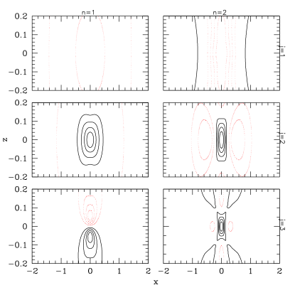
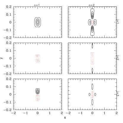
Figure 3: Six orthogonal potential and density pairs (left and right panels, resp.) labeled by vertical index $j$ and radial index $n$. Azimuthal order is $m=0$. Five contour levels are linearly spaced from from zero to the largest absolute peak value. Positive (negative) levels are shown as solid (dotted) lines.

Since the SLE solution is a good match to the radial profiles, we only need the empirical transformation in the $z$-direction. As an example of these new functions, Figure 3 shows the first three two-dimensional orthogonal functions for the two lowest radial orders based on a Monte Carlo realization of the exponential disk with unit scale length and scale height 1/10 using $10^{5}$ particles. Following the symmetry of the equilibrium model, the adaptive algorithm creates the lowest order modes with even symmetry about the disk midplane. However, the four or five lowest-order functions represent enough of the odd component to follow the evolution (cf. Fig. 3).

To summarize, the algorithm for the n-body force calculation for the three-dimensional cylindrical basis is then as follows:

1. Compute $S_{\mu\nu}$ from particle distribution using the basis derived from equation (2.2) with $Z(z)$ chosen as discussed above.

2. Compute transformation to new basis by solving for the eigenvectors.

3. Retain eigenvectors corresponding to the $M$ largest eigenvalues. The value of $M$ may either be predetermined or computed adaptively from the cumulative distribution of eigenvalues (see Weinberg 1996 for details).

4. Tabulate the new orthogonal set and use this to evaluate force for some time-interval on order of a dynamical time for the problem of interest.

5. Goto 1.

The computational bottleneck in this procedure is the construction of $S_{\mu\nu}$ and computing Steps 1–3 can be a significant fraction of the integrated time to advance the particles using the tabulated orthogonal functions for several hundred time steps (30% of the total for the case illustrated in Fig. 3). Nonetheless, the overall force evaluation is still very fast compared to other methods.

Although the underlying trigonometric basis is bounded vertically from above and below, the boundary can be chosen large enough to permit arbitrarily large vertical distortions. Large vertical boundaries require more wavenumber to achieve a fixed resolution. In turn, more wavenumbers affect the computational overhead in computing the empirical basis but do not add to the CPU time required for the force evaluation itself. Therefore, large vertical boundaries remain practical as long as the transform to the empirical basis described in the algorithm above can be done infrequently.

3.2.2 Examples

Figure 4: First five density functions for $m=0$ (left) and $m=1$ (right) with $k=2\pi/5$ ordered from bottom to top. The dotted curve on the lower-left-most panel shows the background exponential disk for comparison.

Figure 5: Expansion coefficient amplitudes for an exponential disk with $\mathop{\rm sech}\nolimits^{2}(z)$ vertical profile as a function of radial order and vertical wavenumber.

Here we build a basis set that closely matches the typical exponential disk profile. As described in §2.2, we adopt an axisymmetric separable density profile, $\rho(r,z)=\rho_{r}(r)\rho_{z}(z)$, chosen to match the background, $\rho_{r}(r)=\rho_{o}(r)$. For this test, $\Psi_{o}\equiv-1/\sqrt{1+(r/a)^{2}}$ takes care of the boundary conditions. Recall that $\Psi_{o}$ and $\rho_{o}$ are not required to satisfy the Poisson equation; equation (7) guarantees that the resulting basis functions will be orthogonal regardless. The results are shown in Figure 4 for the four lowest radial terms for $m=0$ and $1$. The exponential scale length $a=1$ and vertical boundary $L=10$ is chosen to represent a disk with scale length to scale height ratio of 10:1. The wavenumbers are $k=2\pi j/Lj,j=0,1,\ldots,j_{max}$ for pill box of half-height $L$. The density functions in the figure have $k=2\pi/5$ ($j=2$). The lowest order $m=0$ case is compared with the exponential disk (dotted). For large $k$, the lowest order radial function falls off more rapidly than the exponential disk. However, the series converges quickly in radial order and wavenumber as demonstrated in Figure 5 which shows the coefficients for an expansion of Monte Carlo realization of an exponential disk with $\rho_{z}\propto\mathop{\rm sech}\nolimits^{2}(z)$. Good agreement demonstrates that satisfactory results are obtained without exact Poisson solutions $\rho_{o}$ and $\Phi_{o}$. The biorthogonality condition (eq. 13) is good to one part in $10^{9}$.

The grid points for the Sturm-Liouville solution described in §2.3 are chosen by mapping the semi-infinite interval to the segment $[-1,1]$ using $x=(r-1)/(r+1)$ and choosing points evenly spaced in $x$. The Pruess & Fulton algorithm can estimate the grid automatically to optimize accuracy but this mapping provided sufficiently high-accuracy and rapid execution.

I checked accuracy and consistency of the final basis set by evaluating the gravitational force for a Monte Carlo distribution of $10^{5}$ bodies with the proposed method and with a direct summation. Contours of constant force are better than $1\%$ except where the direct summation evaluation is badly affected by discreteness noise.

4 Summary and conclusions

This paper presents a numerical algorithm for constructing biorthogonal expansion bases for use in n-body force calculation and linear perturbation theory and explores its performance. The major results of this investigation are as follows:

1. This algorithm removes one of the remaining limitations of the self-consistent field (SCF) method by providing basis sets tailored to any background galaxian profile.

2. The algorithm is applicable to any separable coordinate system. This paper details and benchmarks its implementation for spherical and three-dimensional cylindrical bases.

3. Sturm-Liouville equation solvers are publically available (e.g. see Pruess & Fulton 1993 for Fortran code) and a desired basis is readily obtained using equations (10)–(12).

4. The main limitation of this method for n-body codes is the necessity to tabulate the basis functions rather than derive them from recursion relation on the fly (as in Clutton-Brock 1973 and Hernquist & Ostriker 1992). On the other hand, this is largely a programming inconvenience; the algorithm is still easily parallelized and the table lookup is not a computational bottleneck.

5. For spherical expansions, the algorithm is conceptually equivalent to and computationally competitive with the published SCF expansions. For three-dimensional cylindrical expansions, the coupling of the vertical and radial parts of the potential-density pairs requires an additional orthogonalization step. This increases the computational overhead by up to 50% but does not effect scaling with particle number or parallelizability.

6. The use of these basis sets is not limited to n-body simulation. They are easily used in semi-analytic linear perturbation calculations and, moreover, facilitate the comparison between the n-body and perturbation theory.

References

- (1) Allen, A. J., Palmer, P. L., and Papaloizou, J. 1990, MNRAS, 243, 576.
- (2) Clutton-Brock, M. 1972, Astrophys. Space. Sci., 16, 101.
- (3) Clutton-Brock, M. 1973, Astrophys. Space. Sci., 23, 55.
- (4) Courant, R. and Hilbert, D. 1953, Methods of Mathematical Physics, Vol. 1, Interscience, New York.
- (5) Earn, D. J. D. 1996, ApJ, 465, 91.
- (6) Earn, D. J. D. and Sellwood, J. A. 1995, ApJ, 451, 533.
- (7) Eastwood, J. W. and Brownrigg, D. R. K. 1979, J. Comput. Phys., 32, 24.
- (8) Fridman, A. M. and Polyachenko, V. L. 1984, Physics of Gravitating Systems, Vol. 2, p. 282, Springer-Verlag, New York.
- (9) Hernquist, L. 1990, ApJ, 356, 359.
- (10) Hernquist, L. and Ostriker, J. P. 1992, ApJ, 386, 375.
- (11) Hernquist, L., Sigurdsson, S., and Bryan, G. L. 1995, ApJ, 446, 717.
- (12) Kalnajs, A. J. 1976, ApJ, 205, 745.
- (13) Marletta, M. and Pryce, J. D. 1991, Comp. Phys. Comm., 63, 42.
- (14) Pruess, S. 1973, SIAM J. Numer. Anal., 10, 55.
- (15) Pruess, S. and Fulton, C. T. 1993, ACM Trans. Math. Software, 63, 42.
- (16) Pryce, J. D. 1993, Numerical Solution of Sturm-Liouville Problems, Oxford.
- (17) Saha, P. 1993, MNRAS, 262, 1062.
- (18) Weinberg, M. D. 1990, Baryonic Dark Matter, Chapt. Wide Binaries and Mass Limits on Dark Matter, pp 117–136, Kluwer Academic Publishers, Netherlands.
- (19) Weinberg, M. D. 1996, ApJ, 470, 715.
- (20) Weinberg, M. D. 1997, MNRAS, in press.