A Deep VLA survey at 20cm of the ISO ELAIS survey regions

Abstract

We have used the Very Large Array(VLA) in C configuration to carry out a sensitive 20cm radio survey of regions of sky that have been surveyed in the Far Infra-Red over the wavelength range 5-200 microns with ISO as part of the European Large Area ISO Survey(ELAIS). As usual in surveys based on a relatively small number of overlapping VLA pointings the flux limit varies over the area surveyed. The survey has a flux limit that varies from a 5$\sigma$ limit of 0.135mJy over an area of 0.12deg² to a 5$\sigma$ limit of 1.15mJy or better over the whole region covered of 4.22 deg². In this paper we present the radio catalogue of 867 sources. These regions of sky have previously been surveyed to shallow flux limits at 20cm with the VLA as part of the VLA D configuration NVSS(FWHM=45 arcsec) and VLA B configuration FIRST(FWHM=5 arcsec) surveys. Our whole survey has a nominal 5 sigma flux limit a factor of 2 below that of the NVSS; 3.4 deg² of the survey reaches the nominal flux limit of the FIRST survey and 1.5 deg² reaches to 0.25 mJy, a factor of 3 below the nominal FIRST survey limit. In addition our survey is at resolution intermediate between the two surveys and thus is well suited for a comparison of the reliability and resolution dependent surface brightness effects that affect interferometric radio surveys. We have carried out a a detailed comparison of the reliability of our own survey and these two independent surveys in order to assess the reliability and completeness of each survey.

1 Introduction

The Infrared Space Observatory (ISO, Kessler et al. 1996), launched in November 1995 was the successor of the Infrared Astronomical Satellite (IRAS) and provided unparallel sensitivity in mid to far infrared wavelengths ($i.e.$ 5–200 $\mu m$). The European Large-Area ISO Survey (ELAIS, Oliver et al. 1997, Oliver et al. 1998 in preparation) is a project that used ISO to carry out a deep wide angle survey at wavelengths of 6.7, 15, 90 and 175 $\mu m$. The 6.7 and 15 $\mu m$ surveys were carried out with the ISO-CAM camera (Cesarsky et al. 1996) with the aim to reach a 5$\sigma$ sensitivity of $\sim$2mJy at 15microns. The $90\mu m$ and 175$\mu m$ surveys used the ISO-PHOT camera (Lemke et al. 1994) with the aim to reach a 5$\sigma$ sensitivity of $\sim$25mJy. At these limits, we expect ISO to be confusion limited at 90 $\mu m$ and 175 $\mu m$ by galaxies and galactic cirrus emission and hence this survey should be the deepest FIR survey possible with the satellite.

The area covered in the ELAIS survey is $\sim 13$ square degrees at 15 and 90 microns, $\sim 7$ square degrees at 6.7 microns and $\sim 3$ square degrees at 175microns.

The ELAIS survey is $\sim$50 times deeper at 5-20$\mu m$ than IRAS. Thus our survey will allow us to explore IRAS-like populations to higher redshift and possibly unveil new classes of objects or unexpected phenomena. We expect to detect thousands of galaxies, many of which will be at high redshifts and undergoing vigorous star formation. The expected large number of high-z IR galaxies should provide vital information about the star formation rate out to z=1 and possibly earlier.

The spatial resolution of ISO will be insufficient to properly identify optically faint objects. At 15 microns, the survey resolution is $\sim$ 10 arcsec and at 90 microns it will be about one arc minute. Complementary radio data will play a crucial role in identifying many of the most interesting objects, as they did in the early days of X-ray astronomy (e.g. Cyg X-1) and in more recent times for IRAS (e.g. IRAS F10214+4714 (Rowan-Robinson et al. 1991).

In this paper we report the description of the radio observations obtained in the three ISO-ELAIS survey regions in the northern celestial hemisphere (N1_1610+5430, N2_1636+4115 and N3_1429+3306). The observations are made with the Very Large Array (VLA) radio telescope at 1.4GHz (20cm) in the VLA C-configuration (maximum baseline 11km) with a resolution (FWHM) of $\sim 15$ arcsec. The aim of these VLA observation was to obtain an uniform covering of the ELAIS regions with a rms noise limit of $\sim$50 $\mu$Jy. These VLA observations will be essential in the optical identification phase of the ELAIS sources and in assessing the reliability of the ELAIS source lists.

Moreover, with a radio survey it will be possible to investigate the radio/far–infrared correlation in star forming galaxies to flux densities deeper than those reached by IRAS. Helou, Sofier & Rowan-Robinson (1985) noted a strong correlation between radio and far infrared flux for star forming galaxies, valid over a very wide range of infrared luminosities, and this has been confirmed in many other studies (e.g. Wunderlich, Klein & Wielebinski 1987; Condon, Anderson & Helou 1991). The radio emission is interpreted as a synchrotron radiation from relativistic electron which have leaked out of supernova remnants. It is expected that this correlation should extend below the IRAS flux level since the majority of the sub-mJy radio sources have been identified with faint blue galaxies whith spectra similar to those of star forming objects (Benn et al. 1993).

In addition, combining deep radio and optical data with the ISO survey fluxes will provide information on the trivariate IR-radio-optical luminosity function and its evolution and the contribution of starburst galaxies to the sub-mJy radio source counts. The ratio of the FIR emission and radio emission will also allow is to investigate the physical origin and spatial distribution of the energy sources in the detected objects in the same way that VLA maps have been central to our understanding of the origin of IRAS sources.

Finally, this survey, due to its depth and extension, is very important also as radio survey in its own right. In fact, the selected sample is large and deep enough to constitute a statistically significant sample of sub-mJy radio sources, whose nature and characteristics are still a major topic in observational cosmology (see Windhorst, Mathis & Neuschaefer 1990, Fomalont et al. 1991, Rowan-Robinson et al. 1993, Gruppioni et al. 1997)

2 Radio observations

2.1 Choice of observing frequency and VLA configuration

The VLA C–configuration and the observing frequency of 1.4 GHz give the optimum resolution to acquire the kind of radio data that we need. Whilst less prone to surface brightness effects , the VLA D configuration is confusion-limited at the fluxes we wish to attain (the 5 $\sigma$ confusion limit in D configuration is 0.4 mJy/beam). With the C configuration and a frequency of 1.4 GHz the synthesized beam size (Full Width at Half Power, FWHP) is $\sim$15 arcsec. The well-defined synthesized beam of the VLA should enable us to pinpoint optical identifications to 1 arcsec, except for the asymmetric multi-components sources. The frequency of 1.4 GHz was chosen because at this frequency the FWHP of the VLA primary beam is 31 arcmin. This allow us to cover the ELAIS field with a relative small number of pointing centers. In fact it is possible to obtain a mosaic map with nearly uniform sensitivity if the separation is 31 / $\sqrt{2}$ $\sim$ 22 arcmin. Moreover, at 1.4 GHz there will be contributions from both the steep and flat spectrum population of radio sources.

Figure 1: The sky position and orientation of the ISO survey regions. Each outer rectangle is 120${}^{\prime}\times 80^{\prime}$. The triangles show the ISO CAM pointings, while the asterisk show the ISO PHOT pointings. The circles show the regions we mapped with the VLA. The circles are drawn with radii R$=20^{\prime}$, where the VLA power sensitivity is $\sim$30% of the central value. The thick circle in N2 is the deep pointing N2 VD (see text for more details).

Our observations are made in spectral line mode using two different IF channels centered at 1.3649 GHz (IF1) and 1.4352 GHz(IF2). Each IF channel has a bandwidth of 18.75 MHz, which is subdivided into 7 spectral line channels evenly spaced in frequency across the bandwidth of the input IF channel. Therefore, we have a total of 14 spectral line channels (7 for each IF) with a bandwidth of 2.68 MHz each. We decided to use the line mode in order to facilitate wide field mapping and avoid the effect of interference. The total bandwidth available is thus 37.5 MHz, narrower than the 50MHz used in continuum mode. A narrower bandwidth means a worse sensitivity. In our case we lose about $\sim$25% in sensitivity or 15% in signal to noise near the pointing centers because the total bandwidth is 75% of that in the continuum mode. However, we considerably reduce the chromatic aberration (bandwidth smearing), which reduces the area covered by each pointing in continuum mode. In addition, the line mode is less susceptible to narrow interference noise spikes, since one only needs to excise the channel that is affected rather than loosing the whole IF band, which is the case in continuum mode. Since our aim is to obtain an uniform sensitivity over the whole ELAIS fields and not to obtain a single-field deep survey, we have opted to use the line mode. Moreover, the reduced bandwidth smearing in line mode will give us more accurate angular sizes for our sources.

2.2 Observations

The VLA observation of the ELAIS regions were carried out in April 96 (10 hours) and in July 1997 (24 hours). A total of 20 pointings were made in 20cm spectral line mode. Seven of these pointings are in the ELAIS field N1, eight in the field N2 and five in N3. The integration time of each pointing was $\sim$ 1 hour. This allowed us to obtain, in each field, a root mean square (rms) noise of $\sim$ 0.05 mJy (a 5 $\sigma$ limit of 0.25 mJy). Moreover, during the July 1997 run, we observed two regions (one in N1 and one in N2) with an integration time of $\sim$ 3 hours each. In particular, in N1 we re-observed (for $\sim$ 3 hours) the pointing V1 (already observed for one hour in April 1996) while in N2 the deep pointing (N2 VD) was shifted of 10 arc min from the map center to avoid the presence of a strong ($>$100 mJy) radio source. In the two deep pointings N1 V1 and N2 VD we reached an rms noise of $\sim$ 0.026 mJy (a 5 $\sigma$ limit of 0.13 mJy). Finally, in order to study the degradation of the image quality as the off-axis of the sources increase, a strong calibrator (the source 3C286) was observed at position offset of 5,10,15,20,25,30 and 35 arcmin in two orthogonal directions (North-South and East-West). The result of this test is reported in section  5.1.2.

In Table 1 we report the position of the center of each observation, while Figure 1 shows the sky position and orientation of the ISO survey regions. The circles show the VLA regions mapped. The circles are drawn with a radius (R$\sim 20^{\prime}$) where the VLA power sensitivity is $\sim$30% of the central value.

Table 1: VLA Observations of ELAIS regions

Region	Pointing	Observing	RA	DEC	Integration	Theoretical	Observed
		Data	(J2000)	(J2000)	Time (min)	rms (mJy)	rms (mJy)
N1	V1	April 96	16 10 00.00	+54 30 00.00	58.4	0.052	0.049
N1	V1	July  97	16 10 00.00	+54 30 00.00	175.4	0.030	0.030
N1	V2	July  97	16 09 25.51	+54 06 32.42	57.8	0.052	0.050
N1	V3	July  97	16 07 34.62	+54 25 05.31	58.5	0.052	0.051
N1	V4	July  97	16 08 09.65	+54 49 08.14	59.5	0.052	0.052
N1	V5	July  97	16 10 37.76	+54 54 36.12	59.0	0.052	0.049
N1	V6	July  97	16 12 28.43	+54 35 55.56	59.0	0.052	0.051
N1	V7	July  97	16 11 51.23	+54 11 54.45	57.8	0.052	0.052
N2	V1	April 96	16 36 00.00	+41 06 00.00	65.3	0.050	0.050
N2	V2	April 96	16 34 00.00	+41 06 00.00	56.8	0.053	0.052
N2	V3	April 96	16 38 00.00	+41 06 00.00	59.3	0.052	0.050
N2	V4	July  97	16 37 00.00	+40 46 00.00	59.2	0.052	0.052
N2	V5	July  97	16 37 00.00	+41 26 00.00	59.0	0.052	0.052
N2	V6	July  97	16 35 00.00	+40 46 00.00	59.5	0.052	0.053
N2	V7	July  97	16 35 00.00	+41 26 00.00	59.5	0.052	0.051
N2	VD	July  97	16 35 00.00	+41 06 00.00	178.4	0.030	0.050
N3	V1	April 96	14 28 30.00	+33 20 00.00	56.5	0.053	0.053
N3	V2	April 96	14 26 30.00	+33 20 00.00	58.7	0.052	0.053
N3	V3	July  97	14 27 30.00	+32 58 30.00	58.9	0.052	0.052
N3	V4	July  97	14 30 30.00	+33 20 00.00	59.5	0.052	0.050
N3	V5	July  97	14 29 30.00	+32 58 30.00	58.0	0.052	0.051

3 Data Reduction

All the data were analyzed with the NRAO AIPS reduction package. The data were calibrated using 3C286 as primary flux density calibrator (assuming a flux of 15.04 Jy at 1.3649 GHz (IF1) and 14.70 Jy at 1.4352 GHz (IF2)) and the sources 1549+506 and 1635+381 as secondary calibrators. The task UVFLAG was used to “flag” (delete) the corrupted data ($e.g.$ bad integration, non operating antennas, high amplitudes due to interferences $etc$) while the tasks VLACALIB and GETJY were used to calibrate the data and to determine the source flux densities. Finally each observation was cleaned using the task IMAGR.

3.1 Root mean square (rms) map noise of the single pointings

The integration time of each observation after deletion of the corrupted data are reported in Table 1. The rms noise of each pointing was estimated using the amplitude distribution of the pixel values in the cleaned map before correcting for primary-beam attenuation. In Figure 2 we show this distribution for the pointing N2 V1. This distribution is the sum of a Gaussian noise core with a positive-going tail caused by discrete sources. Note that the y-axis in Figure 2 is logarithmic.

Thus the rms of the noise distribution alone should be nearly equal to the rms of that distribution obtainable by reflecting the negative flux portion of the observed amplitude distribution about flux=0. In column VII of Table 1 we report the theoretical rms noise level (at 1$\sigma$) as computed directly from the observing parameters (integration time, number of antennas, observing frequency, bandwidth and number of $IF$ channels), while in column VIII we report the 1$\sigma$ rms noise level obtained by fitting the noise distribution of each pointing. As shown in Table 1 there is a very good agreement between the observed and the theoretical rms noise levels.

Figure 2: Logarithmic histogram of VLA map peak flux densities in the pointing N2 V1

3.2 Mosaic maps

Figure 3: Central 26$\times$26 arcmin² = 520$\times$520 pixels of the mosaic map N1. The contour level are 0.25,0.50,0.75,1.00, 1.25 … mJy. The noise at the corners of the image (see for example the low right corner) is due to the increase of the rms noise as the off-axis value increase

Using the AIPS task LGEOM, HGEOM and LTESS we have combined all the observations and we have created a mosaic map for each field (N1, N2 and N3). A special procedure has been adopted for N2. The presence of a deep observation not in the center of the radio map (see above and Figure 1) makes the noise of this map strongly irregular. To simplify the extraction of the sources we have created two different mosaic maps. In the first map we have combined all the observation in N2 excluding the deep pointing, while in the second one we have combined the deep pointing N2 VD with all the surrounding pointings (N2 V1, N2 V2, N2 V6 and N2 V7, see Figure 1). In this way we have obtained two mosaic maps with a regular noise: lower in the map center and higher in the outer regions.

An example of our map is given in Figure 3 where we show the contour map of the central region (26$\times$26 arcmin²) of the mosaic map N1.

3.3 Noise of the mosaic maps

We analyzed the noise properties in each mosaic maps (N1, N2, N2 Deep and N3). As expected, N1, N2 and N2 Deep have a regular noise distribution: a circular central region with a flat noise surrounded by concentric annular region, where the noise increases for increasing distance from the center (the off-axis value). No structures or irregularities were found in the rms maps. In Figure 4 we plot the variation of the rms as function of the off-axis value for N1, N2 and N2 Deep. Due to the different number of pointings in N3 (five pointings instead of seven, see Figure 1) the mosaic map in this field has a different shape and the noise distribution in the map has a semi-circular shape instead of a circular one. In Figure 4d,e,f we plot the variation of the rms value in three different slices. In Figure 4d we plot the rms in the North-South direction, in Figure 4e the rms in a slice that connects the center of the three northern pointings (N3 V1, N3 V2 and N3 V4), while in Figure 4f we report the rms value in a slice that connects the center of the two souther pointings (N3 V3 and N3 V5). As for N1 and N2, no structures or irregularities were found in the rms map of N3.

Figure 4: The rms noise value as function of the off-axis value. The solid line represent an rms value of 0.05 mJy. See text for more details.

4 Source Catalogue

4.1 Regions for the source extraction

Using Figure 4 we determined the regions with constant rms noise to be used for the source extraction. Due to the circular shape of the rms map, we searched for radio sources in a circular central region plus concentric annular regions to an off-axis value of 42 arcmin. Outside this area, the beam attenuation significantly increases the limiting flux (see Figure 4). In each region the rms used for source extraction is the highest rms in the region. In this way we are sure that all the sources extracted are above the fixed threshold in the region (for example 5 times the rms value). The sizes of these regions are reported in Table 2 and in Figure 5.

Using the data reported in Table 2 we obtained the solid angle $\Omega(S_{p})$ as function of the peak flux density $S_{p}$ covered by our survey. This effective survey area is shown in Figure 6.

Table 2: The regions used for the sources extraction

Region	Rinn	Rout	Size	Total	rms	5 $\sigma$ limit
	($\prime$)	($\prime$)	deg2	deg2	mJy	mJy
N1
1	0	8	0.0559	0.0559	0.027	0.135
2	8	14	0.1151	0.1710	0.034	0.170
3	14	22	0.2513	0.4223	0.038	0.190
4	22	26	0.1677	0.5900	0.050	0.250
5	26	30	0.1955	0.7855	0.070	0.350
6	30	34	0.2234	1.0089	0.100	0.500
7	34	38	0.2513	1.2602	0.150	0.750
8	38	42	0.2793	1.5395	0.230	1.150
N2
1	0	26	0.5900	0.5900	0.050	0.250
2	26	30	0.1955	0.7855	0.070	0.350
3	30	34	0.2234	1.0089	0.100	0.500
4	34	38	0.2513	1.2602	0.150	0.750
5	38	42	0.2793	1.5395	0.230	1.150
N2 D
1	0	8	0.0559	0.0559	0.027	0.135
2	8	11	0.0497	0.1056	0.030	0.150
3	11	14	0.0655	0.1711	0.038	0.190
N3
1	0	26	0.2950	0.2950	0.050	0.250
2	26	30	0.1645	0.4595	0.070	0.350
3	30	34	0.1961	0.6556	0.100	0.500
4	34	38	0.2279	0.8835	0.150	0.750
5	38	42	0.2597	1.1432	0.230	1.150

Figure 5: The region used for the source extraction. The lines with the same thickness enclose regions with the same rms noise value (see Table 2)

Figure 6: Solid angle over which a source with detected peak flux density S_p can be counted.

4.2 Source detections

Within each region we searched for radio sources up to a peak flux density $\geq$ 5 times the rms value of the region. The sources were extracted using the task SAD (Search And Destroy) which attempts to find all the sources whose peaks are brighter than a given level. For each selected source the flux, the position and the size are estimated using a least square Gaussian fit. However, for faint sources a Gaussian fit may be unreliable (see Condon 1997, for an extensive discussion about errors in Gaussian fits). For this reason we decided first to run the task SAD with a flux limit of 3 times the local rms value (see Table  2). Subsequently, we derived the peak flux of faint sources (those detected with $3\sigma<S_{peak}<7\sigma$) using a second degree interpolation (task MAXFIT). Only the sources with a MAXFIT peak flux density $\geq$ 5 $\sigma$ were included in the sample. For these faint sources the total flux density was obtained using the task IMEAN, which integrates the map value in a specific rectangle, while for all the other parameters (major axis, minor axis and position angle) we used the values obtained with the Gaussian fit. For irregular resolved sources the total flux density was calculated using the task TVSTAT which allows us to use an irregular area to integrate the map value.

4.3 Multiple sources

Detected sources separated by less than two times the value of our synthesized beam size ($i.e.$ 25 arcsec) and with a flux ratio lower than 2 have been considered as an unique source. We adopted this criterion because the component flux density ratio of physically doubles is usually small (${{}_{<}\atop{}^{\sim}}$2) while the projection pairs can have arbitrarily large flux density ratio (Condon, Condon and Hazard, 1982).

5 The Source Catalogue

Considering all the available observations we detected a total of 867 sources at $\geq$ 5 $\sigma$ level (44 of which have multiple components) over a total area of 4.222 deg². The catalogue with all the 867 sources (921 components) reports the name of the source, the peak flux density S_P in mJy, the total flux density S_I in mJy, the RA and DEC (J2000), the full width half maximum (FWHM) of the major and minor axes $\theta_{M}$ and $\theta_{m}$ (in arcsec), the positional angle PA of the major axis (in degrees) and the off-axis values in the VLA map (in arcmin). The different components of multiple sources are labeled “A”, “B”, etc., followed by a line labeled “T” in which flux and position for the total sources are given. For these total sources the position have been computed as the flux-weighted average position for all the components. Table 3 shows the first page of the catalogue as an example.

In Table 4 we report the number of radio sources detected in N1, N2 and N3, while in Figure 7 we show the distribution of the peak flux density and the total to peak flux ratio as a function of peak flux for all the 867 sources. Contour maps of all the 44 double or multiple sources are shown in Figure  8  9 and  10.

Figure 7: Peak flux distributions (upper) and total to peak flux ratio as function of peak flux (lower) for all the radio sources detected in N1, N2 and N3

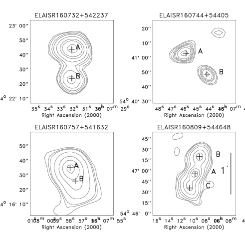
Figure 8: SMALL EXAMPLE (This figure is available in its entirety in http://www.ast.cam.ac.uk/$\sim$ciliegi/elais/papers/) : Contour maps for multiple sources in N1. Contour levels are 5,6,7,8,10 …. times the local rms noise value (see Table 2) Each map is $1^{\prime}\times 1^{\prime}$ except for very extended sources for which the map size is variable. For these sources the vertical bar in the map shows 1 arcmin.

Figure 9: As in Figure 8 for N2. This figure is available in http://www.ast.cam.ac.uk/$\sim$ciliegi/elais/papers/

Figure 10: As in Figure 8 for N3. This figure is available in in http://www.ast.cam.ac.uk/$\sim$ciliegi/elais/papers/

Table 4: The number of radio sources detected in each field

Field	Single	Multiple	Total
	Sources	Sources	Sources
N1	345	16	361
N2	305	16	321
N3	173	12	185

5.1 Sources parameters and their uncertainties

5.1.1 Positions and angular sizes

Following Condon 1997, the error on the sources parameters reported in the catalogue have been calculated using :

$$\frac{\sigma^{2}_{S_{P}}}{S^{2}_{P}}=\frac{\sigma^{2}_{S_{I}}}{S^{2}_{I}}=\frac{\sigma^{2}_{\theta_{M}}}{\theta^{2}_{M}}=\frac{\sigma^{2}_{\theta_{m}}}{\theta^{2}_{m}}=\frac{\sigma^{2}_{PA}}{2}\left(\frac{\theta^{2}_{M}-\theta^{2}_{m}}{\theta^{2}_{M}\theta^{2}_{m}}\right)^{2}=\frac{2}{\rho^{2}}$$ (1)

where $\rho$ is the signal to noise ratio given by

$$\rho=\frac{\pi}{8ln2}\frac{\theta_{M}\theta_{m}S_{P}}{h^{2}\sigma^{2}_{map}}$$ (2)

Equations 1 and 2 are the master equations for estimating variances of the parameters derived from a two dimensional Gaussian fit on an image with a noise variance $\sigma^{2}_{map}$ and pixel size h. In our maps $h$=3 arcsec, while column 5 of Table  2 reports the value of $\sigma_{map}$ as function of the off-axis value. The rms position error are given by (Condon et al. 1998):

$$\sigma^{2}_{\alpha}=\varepsilon^{2}_{\alpha}+\sigma^{2}_{\theta_{M}}\sin^{2}(PA)+\sigma^{2}_{\theta_{m}}\cos^{2}(PA)$$ (3)

$$\sigma^{2}_{\delta}=\varepsilon^{2}_{\delta}+\sigma^{2}_{\theta_{M}}\cos^{2}(PA)+\sigma^{2}_{\theta_{m}}\sin^{2}(PA)$$ (4)

The mean image off-set $<\Delta\alpha>$, $<\Delta\delta>$ and rms calibration uncertainties $\varepsilon^{2}_{\alpha}$ and $\varepsilon^{2}_{\delta}$ are best determined by comparison with accurate position of sources strong enough that the noise plus confusion terms are much smaller than the calibration terms. We used the 37 single compact sources stronger than 10 mJy found in the $FIRST$ (Faint Images of the Radio Sky at Twenty cm) radio survey (Becker et al. 1997). Their off-sets $<\Delta\alpha>$ and $<\Delta\delta>$ are shown in Figure  11. The mean off-sets of our map are $<\Delta\alpha>=-0.15^{\prime\prime}$ and $<\Delta\delta>=0.18^{\prime\prime}$. The sources coordinate reported in the catalogue (see Table 3) have been corrected for these off-sets.

Figure 11: Position errors for strong point sources (37 sources in our survey and in the $FIRST$ survey with flux radio greater than 10 mJy)

From the distribution of $<\Delta\alpha>$ and $<\Delta\delta>$ shown in Figure  11 we have estimated the rms calibration errors: $\varepsilon_{\alpha}=0.486^{\prime\prime}$ and $\varepsilon_{\delta}=0.351^{\prime\prime}$. Their small values show that our mosaic maps are not affected by relevant geometric distortions due to the approximation of a finite portion of the spherical sky away from the instrumental zenith with a bi-dimensional plane (see Perley 1989, Condon et al. 1998). Using the mean off-sets and calibration errors obtained using the 37 sources stronger than 10 mJy in common with the $FIRST$ survey, we have calculated the positional errors of all our sources. To verify that our positional errors are realistic also for faint sources, we used the 211 single compact sources stronger than 1 mJy found to be in common with the $FIRST$ survey. The right ascension and declination differences $<\Delta\alpha>$ and $<\Delta\delta>$ were divided by the uncertainties $\sigma_{\alpha}$ and $\sigma_{\delta}$ (from Equations 3 and 4). As expected, the normalized error distributions (Figure 12) are Gaussian with nearly zero mean and unit variance, verifying that our positional uncertainties are accurate also for sources down to $\sim$1 mJy.

Figure 12: Position errors for the 211 point sources stronger than 1 mJy in common with the $FIRST$ survey, in unit of the calculated position uncertainties $\sigma_{\alpha}$ and $\sigma_{\delta}$, along with the 90% confidence error circle (upper panel). The smooth curves in the central and lower panel represent the expected Gaussian of zero mean and unit variance.

However, as shown in the flux distribution of Figure 7, the majority of our radio sources have a flux lower than 1 mJy. Since we do not have other radio catalogues below 1 mJy to repeat out test, we decided to use our observations to test the reliability of the position errors down to the flux limit of our survey ($\sim$ 0.135 mJy). In particular, we used the following procedure: (1) Each mosaic map has been obtained combining five or more individual pointings, whose centers are separated by $\sim$ 22 arcmin. (2) Because in each individual map the FWHM of the primary beam is 31 arcmin, there are many overlapping regions where sources are detected in two different pointings. (3) We considered the sources detected in each individual pointing as an independent data set and we used the sources in common ($i.e$ the sources detected in the overlapping regions) to test the reliability of the positional errors. We have a total of 134 sources in the overlapping regions with a flux lower than 1 mJy. The right ascension and declination differences of these 134 sources were divided by the combined errors $\sigma_{RA}$ and $\sigma_{DEC}$, where $\sigma^{2}_{RA}=\sigma^{2}_{\alpha 1}+\sigma^{2}_{\alpha 2}$ and $\sigma^{2}_{DEC}=\sigma^{2}_{\delta 1}+\sigma^{2}_{\delta 2}$ with $\sigma_{\alpha 1},\sigma_{\alpha 2},\sigma_{\delta 1}$ and $\sigma_{\delta 2}$ from Equations 3 and 4. As shown in Figure 13, also these error distributions for faint sources agree with the expected Gaussians (smoothed curves).

Figure 13: Position errors for the 134 point sources in the overlapping region with flux lower than 1 mJy, in unit of the combined position uncertainties $\sigma_{RA}$ and $\sigma_{DEC}$, along with the 90% confidence error circle (upper panel). The smooth curves in the central and lower panel represent the expected Gaussian of zero mean and unit variance.

In conclusion the positional uncertainties obtained using Equations 3 and 4 are accurate also for sources down to the limit of our survey ($\sim$ 0.135 mJy) and they can be used to estimate the reliability of the optical and infrared identifications. The typical rms position uncertainties $\sigma_{\alpha}$ and $\sigma_{\delta}$ are plotted as function of the flux density in Figure  14. The positional errors of the radio sources are $\sim$ 2 arcsec for the fainter sources ($\sim$0.13 mJy) and $\sim$ 0.6 arcsec for the brighter sources ($>$ 10 mJy).

Figure 14: The typical rms position uncertainties $\sigma_{\alpha}$ and $\sigma_{\delta}$ for point sources of flux-density S_peak.

5.1.2 Bandwidth Smearing

The principles upon which synthesis imaging are based are strictly valid only for monochromatic radiation. When radiation from a finite bandwidth smearing is accepted, aberrations in the image will result. These take the form of radial smearing which worsen with increased distance from the center. The peak response to a point sources simultaneously declines in a way that keeps the integrated flux constant. In other words the bandwidth smearing reduces the peak flux density S_P of a source but not its integrated flux density S_I. However, in our case, since we used the spectral line mode where the bandwidth is narrower than in continuum mode, the bandwidth smearing should be negligible. To verify that this is the case, a strong calibrator (the source 3C286) was observed at position offset of 5,10,15,20,25,30,35 arcmin in two orthogonal directions (North-South and East-West) and we made a Gaussian fit of the source in each of the offset position. The ratio between peak and total flux density (S_P/S_I) as function of the off axis value is shown in Figure 15. As shown in Figure 15 the bandwidth smearing is negligible up to r$\simeq$30 arcmin from the center of each single pointing. Therefore the resulting mosaic maps, where the distance between the single pointings is $\sim$ 22 arcmin, are not affected by relevant bandwidth smearing and point sources should have S_P/S${}_{I}>$0.98 everywhere.

Figure 15: Bandwidth smearing reduces the peak flux density S_P of a point sources but preserves the integrated flux density S_I. Abscissa : angular distance from the center (arcmin). Ordinate : The observed ratio S_P/S_I

6 The source counts

The complete sample of 867 sources with $S_{peak}>5\sigma$ was used for the construction of the sources counts. Sources with multiple components are treated as single radio sources. For all the sources we have used the total flux in computing the source counts. Every source was weighted for the reciprocal of its visibility area ($\Omega(S_{p})^{-1}$, see Figure 6) that is the area over which the source could have been seen above the adopted limit. The 1.4 GHz source counts of our survey are summarized in Table 5. For each flux density bin, the average flux density in each interval, the observed number of sources in each flux interval, the differential source density (in sr^-1 Jy^-1), the normalized differential counts $nS^{2.5}$ (in sr^-1 Jy^1.5) with estimated errors (as $n^{1/2}S^{2.5}$) and the integral counts (in sr^-1) are given. The normalized 1.4 GHz counts are plotted in Figure 16 where, for comparison, the differential source counts obtained with other 1.4 GHz radio surveys are also plotted while the integral source counts (deg^-2) are  plotted in Figure 17. The solid line in Figure 16 represents the global fit to the counts obtained by Windhorst, Mathis & Neuschaufer (1990) by fitting the counts from 24 different 1.4 GHz surveys. The open circles represent the counts obtained using the 1.4 GHz survey $FIRST$ (White et al 1997). Finally the open stars represent the 1.4 GHz counts obtained by Gruppioni et al. (1997) in a recent radio survey in the Marano Field (RA=03^h 15^m, DEC=$-$55 13).

As shown in Figure, there is a very good agreement between our counts and those obtained with other surveys. In particular, the points at the fainter flux level confirm the well-know flattening observed in the normalized differential source counts below few mJy (Windhorst, Mathis & Neuschaufer (1990)). The roll-off of the sources in the $FIRST$ survey (open circles in Figure 16) at flux densities less than $\sim$2 mJy is due to the low peak flux densities of many faint, extended sources, which make them undetectable in the $FIRST$ survey. As noted by White et al. (1997) this is a clear indication of the incompleteness of the $FIRST$ survey at the faint limit. On the other hand, the very good agreement between our counts and those obtained with other surveys (also at very faint flux level) and the lack of any roll-off at faint flux level in our counts indicate that our procedure for the source extraction (see above) yields very good results and that our sample is not affected by incompleteness at the faint limit.

A Maximum Likelihood fit to our 1.4 GHz counts with two power laws:

$$\frac{dN}{dS}\propto\left\{\begin{array}[]{ll}S^{-\alpha_{1}}&\mbox{if S $>$ S${}_{b}$}\\ S^{-\alpha_{2}}&\mbox{if S $<$ S${}_{b}$}\end{array}\right.$$ (5)

gives the following best fit parameters: $\alpha_{1}=1.71\pm 0.10$, $\alpha_{2}=2.36\pm 0.20$, $S_{b}\simeq$0.5 mJy. These values suggest that the re-steepening of the integral counts toward an Euclidean slope start below 1 mJy, in agreement with Gruppioni et al. (1997), Condon & Mitchell (1984) and Windhorst, van Heerde & Katgert (1984), while Windhorst, Mathis & Neuschaufer (1990), by fitting the counts of several 1.4 GHz survey, found that the change in slope starts around 5 mJy.

Table 5: The 1.4 GHz Radio Source Counts

$S$	$<S>$	$N_{S}$	$dN/dS$	$nS^{2.5}$	$N(>S)$
(mJy)	(mJy)		sr-1 Jy-1	sr-1 Jy1.5	sr-1
0.13 –   0.23	0.17	87	8.962$\times 10^{9}$	3.60$\pm$  0.39	2.001$\times 10^{6}$
0.23 –   0.42	0.32	188	2.641$\times 10^{9}$	4.61$\pm$  0.34	1.076$\times 10^{6}$
0.42 –   0.76	0.56	148	6.301$\times 10^{8}$	4.78$\pm$  0.39	5.814$\times 10^{5}$
0.76 –   1.36	1.02	127	1.990$\times 10^{8}$	6.56$\pm$  0.58	3.691$\times 10^{5}$
1.36 –   2.46	1.83	112	8.139$\times 10^{7}$	11.68$\pm$  1.10	2.485$\times 10^{5}$
2.46 –   4.42	3.30	64	2.543$\times 10^{7}$	15.86$\pm$  1.98	1.597$\times 10^{5}$
4.42 –   7.96	5.93	53	1.166$\times 10^{7}$	31.61$\pm$  4.34	1.097$\times 10^{5}$
7.96 –  14.33	10.68	43	5.251$\times 10^{6}$	61.87$\pm$  9.43	6.842$\times 10^{4}$
14.33 –  25.79	19.22	17	1.153$\times 10^{6}$	59.07$\pm$ 14.33	3.499$\times 10^{4}$
25.79 –  46.41	34.60	13	4.900$\times 10^{5}$	109.10$\pm$ 30.25	2.177$\times 10^{4}$
46.42 –  83.55	62.27	8	1.675$\times 10^{5}$	162.10$\pm$ 57.31	1.166$\times 10^{4}$
83.55 – 150.39	112.09	5	5.816$\times 10^{4}$	244.70$\pm$109.40	5.443$\times 10^{3}$
150.39 – 270.70	201.77	2	1.293$\times 10^{4}$	236.40$\pm$167.10	1.555$\times 10^{3}$

Figure 16: The normalized differential source counts. The abscissa gives the flux density (mJy) and the ordinate gives the differential number of sources normalized by $S^{2.5}$ (sr^-1 Jy^+1.5). The solid line represents the global fit to the counts obtained by Windhorst, Mathis and Neuschaufer (1990) by fitting the counts from 24 different 1.4 GHz surveys. The open circles represent the counts obtained using the 1.4 GHz survey $FIRST$ (White et al 1997), the filled circles are the counts obtained using our VLA observations in the ELAIS regions while the open stars represent the 1.4 GHz counts obtained by Gruppioni et al. (1997) in the Marano Field.

Figure 17: The integral source counts. The abscissa gives the flux density (mJy) and the ordinate gives the total number of sources per square degree

7 Comparison with the $NVSS$ and $FIRST$ radio catalogues

The regions that we are observing with the VLA are covered also by the $NVSS$ and $FIRST$ radio survey. The $NVSS$ (NRAO VLA Sky Surveys) covers the sky north of J2000 $\delta$=$-40^{\circ}$at 1.4 GHz with $\theta$=45^′′ resolution and nearly uniform sensitivity of 0.45 mJy (1 $\sigma$), while the $FIRST$ (Faint Images of the Radio Sky at Twenty cm) covers over 10,000 squares degrees at 1.4 GHz with a typical 1 $\sigma$ rms of 0.15 mJy and a resolution of 5.4^′′.

It was therefore natural to make a comparison between our results and the results obtained by the $NVSS$ and $FIRST$ surveys on the same regions of the sky.

7.1 SAD on the $NVSS$ and $FIRST$ maps

As first step we used the $NVSS$ and $FIRST$ radio maps to test the reliability of the software that we are using to extract the radio sources (SAD in the AIPS version October 96). From the $NVSS$ and $FIRST$ archive we retrieved the maps covering the region of the sky in the field N2 covered also by the pointing N2 V1, N2 V2 and N2 V3 of our VLA observations (see Table 1).

From the $NVSS$ archive we retrieved the map I1640P40 while from the $FIRST$ archive we retrieved the maps F16330+40417, F16330+41132, F16360+40417, F16360+41132, F16390+40417 and F16390+41132.

Using the software SAD on these maps, we obtained two lists of sources (one for the $NVSS$ and one for the $FIRST$) in the same region covered by our VLA observations. These two lists were compared with the list of sources obtained from the $NVSS$ and $FIRST$ catalogs in which are reported the sources above the $5\sigma$ limits of each survey. The results are reported in Table  6 and in Figure  18.

Table 6: Comparison between SAD and $NVSS$ – $FIRST$ catalogs

SURVEY	Catalogue	SAD	Common	Catalogue	SAD Sources
	Sources	Sources	Sources	Sources	not in Catalogue
				not in SAD
$NVSS$	46	43	43	3	0
$FIRST$	74	70	66	8	4

Figure 18: Ratio of flux reported in the public catalogue to our flux obtained using SAD on the radio map as function of the flux reported in the catalogue for the $NVSS$ (top panel) and for the $FIRST$ (lower panel) surveys

All the three $NVSS$ sources missing in the list obtained by us with SAD have a peak flux density (calculated by us with MAXFIT on the $NVSS$ map) lower than $\sim$ 2.0 mJy ($i.e$ $<$ the 5 $\sigma$ limit of the $NVSS$ maps). Therefore they are probably spurious sources.
Three (163637.9+410511, 163707.5+405125 and 163815.4+405840) of the eight sources present in the $FIRST$ catalogue but not detected by us using SAD on the $FIRST$ map are not detected also in our deeper VLA maps to a flux limit of 0.1 mJy, so they are spurious sources. The other five sources missing in the $FIRST$ list (as well as the four sources detected by SAD but not in the $FIRST$ catalog) have a peak flux density ${{}_{<}\atop{}^{\sim}}$1.2 mJy, i.e. very close to the $FIRST$ flux limit. These differences are probably due to the unreliable Gaussian fit of faint sources as discussed above. Moreover we have to consider that the sources lists (our SAD list and the catalogue lists) are obtained using different source extraction software. In fact, both $NVSS$ and $FIRST$ sources are extracted with special AIPS-based routines wrote exclusively for each survey (see Condon et al. 1993 and White et al. 1997 for more details).

Therefore, in conclusion, we are confident in using SAD as source extraction software, keeping in mind that for faint sources the flux obtained with a Gaussian fit may be unreliable.

7.2 Comparison between our VLA observations and the $NVSS$ and $FIRST$ source catalogues

The primary difficult in comparing the three surveys is the difference in angular resolution. A summary of the main properties of the NVSS, FIRST and our VLA survey is reported in Table 7.

The high resolution surveys will partially resolve extended sources that appear point–like in the low resolution surveys, so that the flux density of the sources will be smaller in $FIRST$ and our survey than in the $NVSS$. To minimize this problem, we restricted the comparison to compact sources ($i.e$ sources with S_I/S${}_{P}<$2) with an off-axis value in our VLA map lower than 34 arcmin. The restriction on the off-axis value allow us to use only the sources detected in regions where the 5$\sigma$ limit is well below the limit of the $FIRST$ survey (see Table 2 and Table 7). For the $NVSS$ and $FIRST$ surveys we used the public source catalogues as available on February 1, 1998.

Table 7: Sensitivity Comparison NVSS, FIRST and our VLA survey

	NVSS	FIRST	Our VLA
			data
VLA Configuration	D	B	C
Beam size	45′′	5′′	15′′
confusion noise	0.08 mJy	0.002 mJy	0.011 mJy
Exposure time	30$-$60 s	3 min	$\sim$1 hour
1$\sigma$ rms noise	0.45 mJy	0.15 mJy	0.05 mJy
5$\sigma$ rms limit	2.25 mJy	0.75 mJy	0.25 mJy

Note: The rms confusion from faint extragalactic source in C-configuration at 20cm is 0.01mJy (Mitchell & Condon, 1985). The value for D-configuration comes from Condon et al. 1998.

Figure 19: The flux obtained with our VLA survey vs. the $NVSS$ flux density as reported in the public catalogue (upper panel) and the ratio of our VLA to $NVSS$ flux density as function of the $NVSS$ flux density (lower panel).

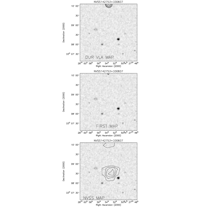
Figure 20: Radio contour plot of the $NVSS$ source NVSS 142753 +330837 present in the NVSS catalogue but not in our VLA and $FIRST$ catalogue overimposed to the optical Digitized Sky Survey (DSS) image. All the maps have a size of 3${}^{\prime}\times 3^{\prime}$. Radio contour level are 0.25,0.35,0.5,0.75,1.0,1.5,1.8,2.5 mJy for our map, 0.75,1.0,1.5,1.8,2.5 mJy for the $FIRST$ maps and 1.0,1.3,1.5,1.7,1.8,2.0,2.2,2.5 mJy for the $NVSS$ map

7.2.1 Our VLA survey versus the $NVSS$ survey

Using the restriction of an off-axis value lower than 34 arcmin and a peak flux density S${}_{P}>$2.3 mJy ($\sim$ the 5$\sigma$ rms limit of the NVSS survey) we have 109 compact sources in common with the NVSS survey. In Figure 19 we show a comparison between our VLA and $NVSS$ total flux densities. A comparison between the flux scales is discussed below. Besides these 109 common sources, there is one $NVSS$ source (NVSS142753+330837) that we did not detected in our survey plus 5 sources (with S${}_{P}>$2.3 mJy) detected in our maps but not in the $NVSS$ survey. In Figure 20 and 21 we report a contour plot of these sources. For comparison a contour plot of the $FIRST$ image in the same region of the sky is also reported. As shown in Figure 20 the $NVSS$ sources missing in our survey is not detected also in the $FIRST$ survey. Its $NVSS$ radio flux is 2.3 mJy, very close to the 5 $\sigma$ detection limit of the survey. It is probably a spurious source but it could be also a very low surface brighteness source detected only in the $NVSS$, the radio survey with the lowest resolution. However a strange phenomenon like a variable radio source can not be completely excluded. For the 5 sources missing in the $NVSS$ survey, Figure 21 clearly shows that one (ELAISR142917+332626) is missing because our higher resolution survey has resolved an extended $NVSS$ source, one (ELAISR142940+330552) is completely undetected on the $NVSS$ map while the other 3 sources are detected also in the $NVSS$ map but below the 5 $\sigma$ limit ($\sim$ 2.25 mJy).

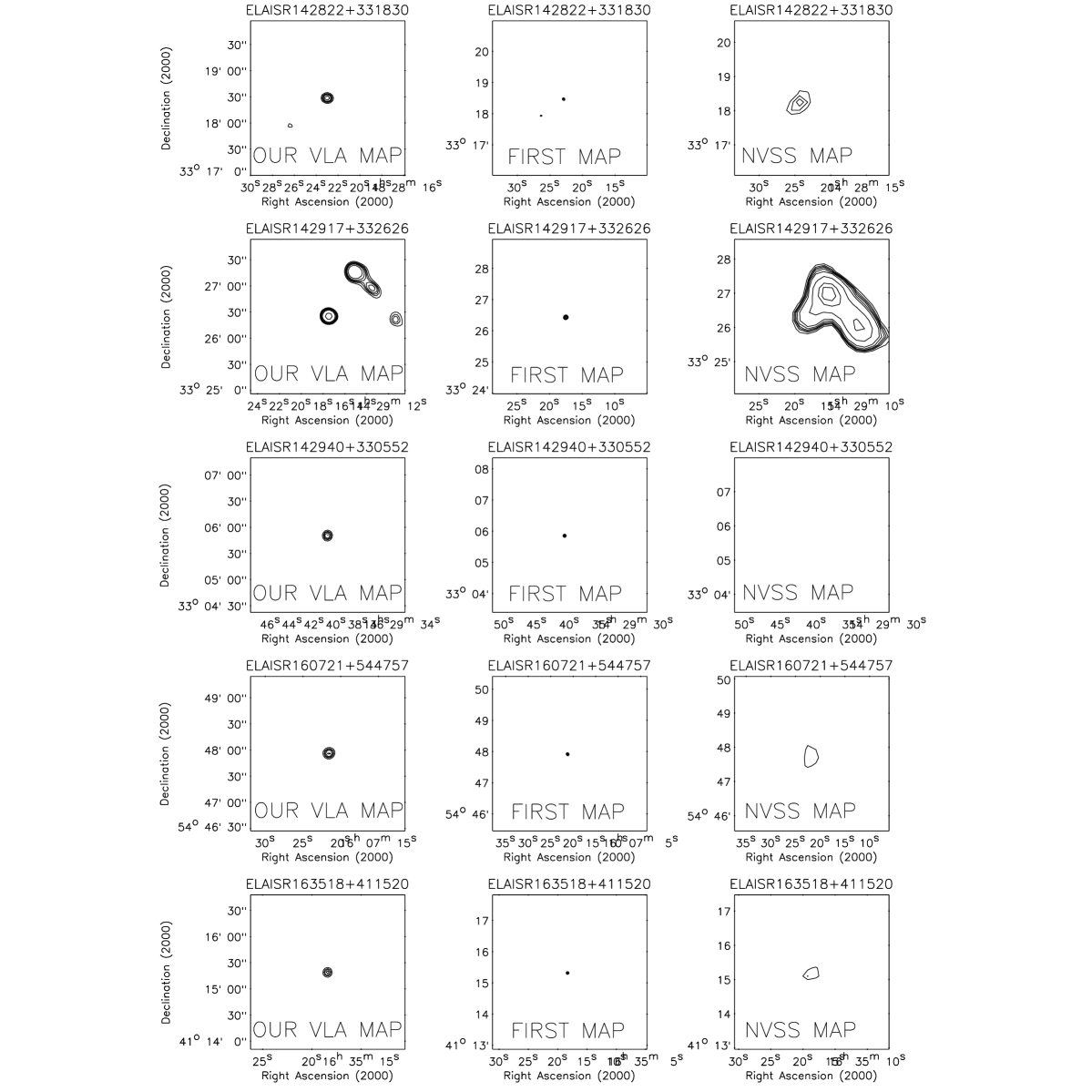
Figure 21: Contour plot of the 5 sources detected in our VLA and $FIRST$ survey but not in the $NVSS$ survey. All the maps have a size of 3${}^{\prime}\times 3^{\prime}$ and a the contour levels of 1.5,1.8,2.0,2.2,2.5,3,5,8 mJy.

All these five sources are present in the $FIRST$ catalogue (and in the $FIRST$ map as clearly showed in Figure 21). Their absence in the $NVSS$ catalogue is an indication of the incompleteness of the $NVSS$ survey near the flux limit.

7.2.2 Our VLA survey versus the $FIRST$ survey

Using the restriction of an off-axis value lower than 34 arcmin and a peak flux density S${}_{P}>$1.0 (the limit of the $FIRST$ catalogue), we have 215 compact sources in common with the $FIRST$ survey. In Figure 22 we show a comparison between our VLA and $FIRST$ total flux densities.

Figure 22: The flux obtained with our VLA survey vs. the $FIRST$ flux density as reported in the public catalogue (upper panel) and the ratio of our VLA to $FIRST$ flux density as function of the $FIRST$ flux density (lower panel).

Besides these 215 common sources, there are 14 $FIRST$ sources that we did not detected in our survey and 29 sources present in our survey but not in the $FIRST$ catalogue. A flux distribution and a contour maps of these last 29 sources are shown in Figure 23 and  24 while a contour maps of the 14 $FIRST$ sources that we did not detect are shown in Figure  24. As shown in Figure 23 all the radio sources missing in the $FIRST$ catalogue have a peak flux density lower than 2 mJy. However, as shown in Figure 24, many of them appear on the $FIRST$ maps. This result confirms the incompleteness of the $FIRST$ survey below $\sim$2 mJy, as already indicated by the differential source counts reported in Figure  5. On the other hand, Figure 24 shows that many of the 14 $FIRST$ sources missing in our survey probably are not real. Some of them may be uncleaned residual around strong sources (see, for example, FIRST161318+541607, FIRST163646+405442, FIRST163815+405840) or simply spurious sources in a not well cleaned map (see, for example, the $FIRST$ maps of FIRST161351+543258, FIRST163634+413013 and FIRST163706+405125).

Figure 23: Flux distribution of the 29 sources detected in our survey with a peak flux density S${}_{P}>$ 1 mJy but not present in the $FIRST$ catalogue

7.2.3 Flux comparison between the three surveys

As shown in Figure 19 and  22 the flux densities of our survey are in good agreement with the $FIRST$ and $NVSS$ flux densities over two order of magnitude. However, as expected, the high resolution surveys tend to estimate lower flux than the lower resolution survey. This effect is evident in the lower panels of Figure 19 and  22 : our VLA flux densities are, in mean, lower than the $NVSS$ flux densities but higher than the $FIRST$ flux densities. High resolution surveys, with their smaller synthesized beam size, lose flux due to the resolution surface brightness effect. However some consideration cam be made from Figure 19 and  22. In spite a factor of 3 in angular resolution between our VLA and $NVSS$ survey (15^′′ vs. 45^′′ FWHM) the flux ratio of the two surveys is always lower than 0.5 while the flux ratio between our VLA and $FIRST$ surveys reaches values of $\sim$ 4, although the two surveys have still a factor of 3 in angular resolution differences (5^′′ vs. 15^′′ FWHM). The missing flux between the $FIRST$ (VLA - B configuration) and our survey (VLA - C configuration) is greater than the missing flux between our survey and the $NVSS$ survey (VLA - D configuration). Therefore the C configuration of our survey with a synthesized beam size of 15^′′ seems to be the better compromise between high (B configuration) and low (D configuration) resolution radio surveys. It is less prone to surface brightness effects than the B configuration without an excessive loss of flux in comparison with the D configuration.

8 Summary

Using the Very Large Array (VLA) radio telescope, we observed at 1.4 GHz a total area of 4.222 deg² in the ISO/ELAIS regions N1 N2 and N3. The lower flux density limit reached by our observation is 0.135 mJy (at 5 $\sigma$ level) on an area of 0.118 deg², while the bulk of the observed regions are mapped with a flux density limit of 0.250 mJy (5 $\sigma$). The data were analyzed using the NRAO AIPS reduction package. The source extraction has been carried out with the AIPS task SAD. The reliability of SAD has been tested using the maps of the radio surveys $FIRST$ and $NVSS$.

Considering all the available observations, we detected a total of 867 sources at 5 $\sigma$ level, 44 of which have multiple components. These sources were used to calculate the normalized differential source counts. They provide a check on catalogue completeness and reliability plus information about source evolution. A comparison with other surveys shows a very good agreement, confirming the presence of the well-know flattening of the counts below 1 mJy, the completeness of our catalogue and the reliability of our procedure for the source extraction.

A comparison with the $FIRST$ and $NVSS$ radio surveys has confirmed the incompleteness of these two surveys near their flux limits, while a flux comparison between the three surveys has shown that our survey with the VLA array in C configuration is the best compromise between high and low resolution radio surveys. The positional errors of the radio sources are $\sim$ 2 arcsec for the fainter sources ($\sim$0.13 mJy) and $\sim$ 0.6 arcsec for the brighter sources ($>$ 10 mJy). This small value will enable us to obtain an accurate and fast optical/infrared identification of the radio sources.

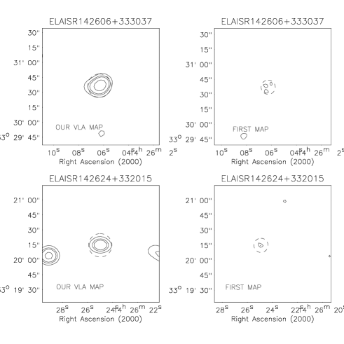
Figure 24: SMALL EXAMPLE (This figure is available in its entirety in http://www.ast.cam.ac.uk/$\sim$ciliegi/elais/papers/) : Contour plot of the sources detected in our VLA survey with a peak flux density S${}_{P}>$ 1 mJy but not present in the $FIRST$ catalogue. The dashed circle shows the position of the source detected in our VLA survey. All the maps have a size of 2${}^{\prime}\times 2^{\prime}$ and a contour levels of 0.50,0.8,1,1.5,2,5,8,10 mJy.

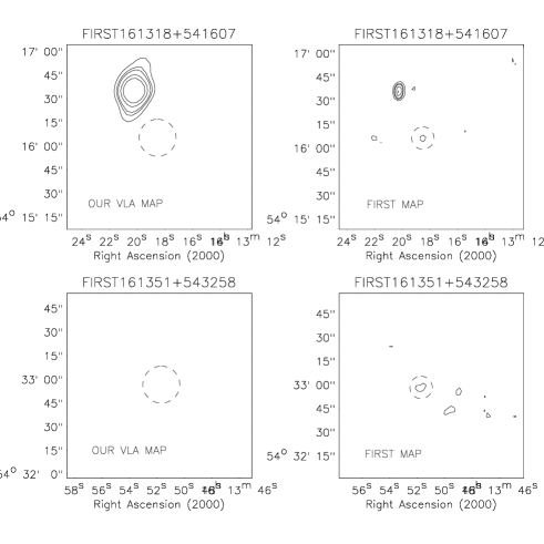
Figure 24: SMALL EXAMPLE (This figure is available in its entirety in http://www.ast.cam.ac.uk/$\sim$ciliegi/elais/papers/): Contour plot of the $FIRST$ source not in our VLA catalogue. The dashed circle shows the position of the $FIRST$ source. All the maps have a size of 2${}^{\prime}\times 2^{\prime}$ and a contour levels of 0.50,0.8,1,1.5,2,5,8,10 mJy.

References

- [1] Benn C.R., Rowan-Robinson M., McMahon R.G., Broadhurst T.J. & Lawrence A., 1993, MNRAS, 263, 98
- [2] Cesarsky et al. 1996, A&A, 315, L32
- [3] Condon J.J., Condon M.A. and Hazard C., 1982, AJ, 87, 739
- [4] Condon J.J. & Mitchell K.J., 1984, AJ, 89, 610
- [5] Condon J.J, Anderson M.L. & Helou G., 1991, ApJ, 376, 95
- [6] Condon J.J, et al., 1993, AAS, 183, 640
- [7] Condon J.J., 1997, PASP, 109, 166
- [8] Condon J.J. et al. 1998, in preparation
- [9] Fomalont E.B.,Windhorst R.A., Kristian J.A. & Kellerman K.I., 1991, AJ, 102, 1258.
- [10] Gruppioni C., Zamorani G., de Ruiter H.R., Parma P., Mignoli M & Lari C., 1997, MNRAS, 286, 470
- [11] Helou G, Sofier B.T. & Rowan-Robinson M., 1985, ApJ, 298, L7
- [12] Kessler M.F. et al. 1996, A&A, 315, L27
- [13] Kleinmann et al., 1988, ApJ, 328, 161
- [14] Lemke D. et al. 1994, ISOPHOT Observer’s manual, ed. U. Klaas, H. Kr ger, I. Heinrichsen, A. Heske, R. Laureijs; Pubs: ESA
- [15] Mitchell K.J. & Condon J.J, 1985,AJ, 90, 1957
- [16] Oliver S. et al. 1997, IAU 179 New Horizons from Multi-Wavelength Sky Surveys, ed: B. McLean; Pubs: Kluwer, in press
- [17] Perley R.A., 1989, in Synthesis Imaging in Radio Astronomy, edit by R.A. Perley, F.R. Schwab & A.H. Bridle (ASP, San Francisco), p. 259
- [18] Rowan-Robinson M. et al. 1991, Nature, 351, 719
- [19] Rowan-Robinson M., Benn C.R., Lawrence A., McMahon R.G. & Broadhurst T.J., 1993, MNRAS, 263, 123
- [20] White R.L., Becker R.H., Helfand D.J. and Gregg M.D, 1997, ApJ, 475, 479
- [21] Windhorst R.A., van Heerde G.M. & Katgert P., 1984,A&AS, 58, 1
- [22] Windhorst R.A., Mathis D.F. and Neuschaefer L.W., 1990, in Kron R.G., ed. ASP Conf. Ser. Vol. 10, Evolution of the Universe of Galaxies Bookcrafters, Provo, p. 389
- [23] Wunderlich E., Klein U. & Wielebinski R., 1987, A&AS, 69, 487