Resolving the Ly$\alpha$ Forest

Abstract

In this paper we critically examine predictions of the Ly$\alpha$ forest within the standard cold dark matter (SCDM) model, paying particular attention to the low end of the column-density distribution. We show in particular that the width of these lines, typically measured by the $b$-parameter of a Voigt profile, is sensitive to spatial resolution in numerical simulations and has previously been overestimated. The new result, which predicts a distribution with a median $b$ of around 20-22 km/s at $z=3$, is substantially below that observed. We examine a number of possible causes of this discrepancy and argue that it is unlikely to be rectified by an increase in the thermal broadening of the absorbing gas, but is instead telling us something about the distribution of matter on these scales. Although the median differs, the shape of the $b$-parameter distribution agrees quite well with that observed, and the high-end tail is naturally produced by the filamentary nature of gravitational collapse in these models. In particular, we demonstrate that lines of sight which obliquely intersect a filament or sheet tend to produce absorption lines with larger $b$ parameters. We also examine the physical nature of the gas which is responsible for the forest, showing that for lines with neutral column densities below $N_{HI}\sim 10^{14}$ cm^-2 (for this model at $z=3$), the peculiar infall velocity is actually slower than the Hubble flow, while larger lines have, on average, turned around and are collapsing.

and

1 Introduction

A physical picture of the Ly$\alpha$ forest in Cold Dark Matter (CDM) dominated cosmologies has recently emerged from numerical simulations (e.g. [Cen et al. 1994]; [Zhang et al. 1995]; [Hernquist et al. 1996]), and other approximation techniques ([Bi 1993]; [Bi & Davidsen 1997]; [Hui, Gnedin & Zhang 1997]; [Gnedin & Hui 1998]). In this context, the absorbers that give rise to low column density lines ($N_{HI}<10^{15}$ cm^-2) at $z\sim 3$ are large, unvirialized objects with sizes of $\sim$ 100 kpc, and low densities, comparable to the cosmic mean ([Zhang et al. 1998]). The width of the lines, as measured by the $b$ parameter of a Voigt profile is set not only by thermal broadening or peculiar velocities, but also by the Hubble expansion across their width ([Weinberg et al. 1997]). In such a situation, there is a monotonic relationship between baryonic density and optical depth which can be exploited to investigate the density distribution along the quasar lines of sight (e.g. [Croft et al. 1998]).

This explanation of the forest (for previous ideas along this direction, see also [Bond, Szalay & Silk 1988], [McGill 1990], [Bi 1993], and [Meiksin 1994]), arising from gravitationally amplified primordial fluctuations, allows us to test various models of cosmological structure formation. This can be done, for example, by comparing the distribution of column densities ([Gnedin 1998]; [Bond & Wadsley 1997]; [Machacek et al. 1998]). These studies have found that the overall normalization of the distribution depends approximately on the parameter $\Omega_{b}^{2}h^{3}/\Gamma$ (there is also some dependence on gas temperature). Here $\Gamma$ is the HI ionization rate, $h$ is the Hubble constant in units of 100 km/s/Mpc, and $\Omega_{b}$ is the ratio of the baryon density to the critical density required to close the universe. For a given model, this parameter is often set by requiring that the mean optical depth match that observed ([Press et al. 1993]; [Zuo & Lu 1993]; [Rauch et al. 1997]). The distribution of column densities is close to a power law and at least approximate agreement seems to be found for a number of popular cosmological models. Another diagnostic is the distribution of $b$ parameters found by fitting Voigt profiles to the spectra. This has been suggested as a probe of the reionization history ([Haehnelt & Steinmetz 1997]).

In this paper, we undertake a systematic evaluation of numerical uncertainties in simulations of the Ly$\alpha$ forest, and in doing so, explore the physical structure of the lines. We will show that the line structure can be rather simply understood, but does require relatively high spatial resolution to model accurately, particularly for the fluctuations at or below the cosmic mean which give rise to the low end of the column density distribution. We cannot address either Lyman-limit or damped Ly$\alpha$ systems as they require more spatial resolution and physical processes than these simulations provide.

The paper is structured in the following way: in section 2, we examine the effect of resolution on various statistical measures of the forest and the gas that gives rise to it, looking first at distributions of density and temperature (section 2.2), and then at the properties of the lines fit to simulated spectra, in section 2.3. We analyze the physical nature of the lines in the next two sections (2.5 and 2.6), other non-parametric measures of the spectra (section 2.7), and the effect of our limited computational volume (section 2.8). Then we discuss these results and the corresponding observations in section 3.

While this paper was in the final stages of preparation, a preprint ([Theuns et al. 1998]) was circulated which examined some of the same issues, although with a different numerical method. Where there is overlap, our results are in agreement. In particular, they also find that the b-parameter distribution requires very high resolution.

2 The effect of spatial resolution

Most of the results for this section come from a set of three simulations in which we modeled the same region of space, but each time increased the resolution by a factor of two. In generating the initial conditions, we keep constant not just the amplitudes but also the phases of the initial conditions (although, of course, higher resolution simulations contain more high-frequency power).

2.1 The simulations

The model is (nearly) the standard Cold Dark Matter (SCDM) model, with total and baryon density parameters $\Omega_{0}=1$ and $\Omega_{b}=0.06$, respectively. The Hubble constant is $h=0.5$ and the matter fluctuation spectrum was normalized to $\sigma_{8}=0.7$, which measures the rms density fluctuations in a tophat sphere of 8$h^{-1}$ Mpc. This normalization is considerably lower than the COBE measured CMB fluctuations would imply, however it is more in line with (although marginally higher than) the value indicated by the number density of large galaxy clusters ([Viana & Liddle 1996]; [White, Efstathiou & Frenk 1993]). We choose this model because it is a standard which we have simulated before ([Zhang et al. 1997]; hereafter known as ZANM97). The power spectrum is realistic enough to produce results which are characteristic of these kinds of hierarchical models, although certainly other parameters can be found which provide a better match to other available observations.

Our box size is 1.2$h^{-1}$ Mpc, too small to include much of the large-scale power important to accurately determine the true distribution of column densities and $b$ parameters, as we will show below (see also [Wadsley & Bond 1997], [Bond & Wadsley 1997]). We adopt such a small volume in order to obtain the highest possible resolution for the lines we do resolve. In other words, we sacrifice the correct distribution of line widths and sizes under the assumption that the internal structure of a given line is not affected by the loss of large-wavelength power. We will show some supporting evidence for this with simulations of larger regions. Three different resolutions are computed, ranging from $32^{3}$ to $128^{3}$ cells, or cell sizes from $37.5h^{-1}$ kpc to $9.375h^{-1}$ kpc.

In order to set this work within the context of other simulations, we show the cell size of some other representative Eulerian Ly$\alpha$ simulations in Table 1, along with all the runs used in this paper. The first three lines are the resolution study runs that will be discussed in the next five sections, while the next five will be used to examine the effect of large-scale power (section 2.8). The gravitational softening length of these simulations is typically 1.5–2 cell widths. Also shown is the Hubble flow across a cell at $z=3$, as well as the size of the box. Of the three simulations by other authors cited in the table, only one ([Zhang et al. 1998]) is of the same cosmological model used in this paper. The other two examined a cosmological-constant dominated cosmology ([Miralda-Escudé et al. 1996]; [Ostriker & Steinhardt 1995]).

Table 1: Selected Eulerian Ly$\alpha$ forest simulations

reference	$\Delta x$ ($h^{-1}$kpc)	$H(z)\Delta x/(1+z)$ at $z=3$ (km/s)	$L_{\hbox{box}}$ ($h^{-1}$ Mpc)
$32^{3}$ (this work)	37.5	7.5	1.2
$64^{3}$ (this work)	18.9	3.8	1.2
$128^{3}$ (this work)	9.4	1.9	1.2
L1.2 (this work)	37.5	7.5	1.2
L2.4 (this work)	37.5	7.5	2.4
L4.8 (this work)	37.5	7.5	4.8
L9.6 (this work)	37.5	7.5	9.6
L4.8HR (this work)	18.9	3.8	4.8
[Zhang et al. 1998] top (sub) grid	37.5 (9.4)	7.5 (1.9)	4.8
[Miralda-Escudé et al. 1996] L10	34.7	4.2	10
[Miralda-Escudé et al. 1996] L3	10.4	1.3	3

We do not include the smoothed-particle hydrodynamics (SPH) simulations since their adaptive smoothing length makes a direct comparison difficult. However we note that the smoothing length of typical SPH simulations scales approximately as the interparticle spacing, which, for Hernquist et al. (1996)her96, is 174 $(\rho_{b}/\left<\rho_{b}\right>)^{-1/3}h^{-1}$ kpc, where $\left<\rho_{b}\right>$ is the mean baryonic density. For the mean density at $z=3$, the Hubble flow across this distance is 34.8 km/s. The gravitational smoothing lengths of SPH simulations are typically much smaller (10 $h^{-1}$kpc for [Hernquist et al. 1996]).

The simulation technique uses a particle-mesh algorithm to follow the dark matter and the piecewise parabolic method (PPM) to simulate the gas dynamics (described in detail in [Bryan et al. 1995]). Since non-equilibrium effects can be important, six species are followed (HI, HII, HeI, HeII, HeIII and the electron density) with a sub-stepped backward finite-difference technique ([Anninos et al. 1997]). We assume a spatially-constant radiation field computed from the observed QSO distribution ([Haardt & Madau 1996] with an intrinsic spectral index of $\alpha=1.5$), which reionizes the universe around $z\sim 6$ and peaks at $z\sim 2$.

As part of the analysis procedure, we generate spectra along random lines of sight through the volume, including the effects of peculiar velocity and thermal broadening of the gas (ZANM97). The spectra are fit by Gaussians (at these column densities, a Voigt-profile is indistinguishable from a Gaussian in optical depth) to obtain column densities and Doppler widths for each line. To match observational samples, a minimum optical depth at line center ($\tau_{HI}=0.05$) is required. The procedure is described in more detail elsewhere (ZANM97), but we go over it briefly here. We neglect a number of observational difficulties; specifically we do not include noise or continuum-fitting. First, maxima in the optical depth distribution are identified as line centers. Then, Gaussian profiles are fit, using a non-linear minimization, to the part of the spectrum which is above $\tau_{HI}=0.05$ and between neighbouring minima. The spectra have a resolution of 1.2 km/s regardless of the spatial resolution of the simulation, a value which is smaller than current observations. We use this technique since we are not interested in a detailed comparison to raw observations, but are more interested in exploring the physical nature of the lines. In other words, we assume that observers have done a good job of correcting their samples for observational biases. Still, we will show (by direct comparison) that the result of not including these observational effects is relatively slight, but only as long as we restrict our comparison to high quality observational samples.

2.2 Physical properties

Figure 1: The distribution of the volume-weighted baryon overdensity at three redshifts ($z=2,3$, and 4) for three simulations with different resolutions.

In Figures 1 and 2, we show the baryonic density and temperature distributions for the three simulations at three redshifts. The density distributions follow the usual approximately log-normal curve (although note the high-density tail), with the majority of the volume below the mean density. This pattern continues at lower redshifts as the voids deepen and the filaments and peaks grow. The difference between resolutions is relatively small, although there is a slight tendency for the higher resolution simulations to have more low-density cells, due both to their additional small-scale power, and to the improved resolution of the small-scale features already present.

The temperature distribution can be described as three features (seen most clearly in the density-weighted distribution). The central one is a peak slightly above $10^{4}$ K, representing dense gas which has collapsed, shock heated and then cooled, generally by line-emission, to this temperature (below which emission processes for our assumed metal-free gas are inefficient). This virialized material is quite dense but occupies a small volume as can be seen by contrasting the volume and density weighted distributions. This means that, although they may be quite prominent in emission features (and indeed would possibly undergo star formation if such processes were included), most of the absorption lines, by number, come from low-density regions that occupy the majority of the volume.

     

Figure 2: The distribution of density-weighted temperature (left panels) and volume-weighted temperature (right panels) at three redshifts each for three resolutions.

The second feature shows up in these plots as a low-temperature shoulder which moves even further to the left at lower redshift. This is low-density gas which was originally heated to $\sim$ 15,000 K by reionization occurring between $z=7$ and 6. It then adiabatically cools with the universal expansion and, because of the low HI fraction and low recombination rate, ionization heating is insufficient after $z\sim 5$ to keep this gas from cooling below $10^{4}$ K. Most of it is below the mean baryonic density.

The third feature is a long, power-law profile of shock-heated material above $10^{5}$ K that is too low-density to cool efficiently. It comes from the halos of clumps, filaments and, in some cases, sheets. The amount of such gas increases with time as longer waves go non-linear, although it is clear that the volume occupied by such gas is extremely small, and will not contribute significantly to the bulk of the Ly$\alpha$ forest. As we will demonstrate in section 2.8, the sharp cutoff at $T\sim 10^{5}$–$10^{6}$ K is due to the artificial lack of large-scale power.

The effect of resolution is again quite small. There are some differences in the high-temperature end, particularly when looking at the mass-weighted statistic, which is due to the improved resolution around small collapsed objects. More interestingly, from the standpoint of the forest, higher resolution systematically produces more low-temperature gas. Such a trend is expected from the change in the density distribution described above: lower density regions are cooler due to enhanced adiabatic expansion and reduced photo-ionization heating.

A better understanding of the effect of resolution can be gained by examining the joint density-temperature relation, shown in Figure 3. The correlation between density and temperature is due to the fact that the thermal history, primarily photo-ionization heating and adiabatic cooling, depends only on density for fluid elements that are not shocked. At higher densities, shocks play more of a role and the correlation is less well-defined. We also show — as a solid line — the analytic equation of state as predicted by Hui & Gnedin (1997), for sudden reionization at $z=6$:

$$T=T_{0}(\rho/\bar{\rho})^{\gamma-1}.$$ (1)

where $T_{0}=10500$ and $\gamma=1.4$. As the resolution is improved, the scatter around this relation increases (we will discuss the reason for this in section 2.6). This is of interest as much semi-analytic work on the forest depends on this relation; however, it should be kept in mind that this is a cell-by-cell plot, and an average over the region that is actually observed as an absorption line will tend to reduce the scatter.

Figure 3: The volume-weighted joint baryon density-temperature distribution for three resolutions at $z=3$. Each point is one cell, subsampled to 8192 points for each panel. The solid line is the predicted equation of state as discussed in the text.

2.3 Line properties

We have seen that there are some, albeit slight, changes to the gross distribution functions of the physical variables in the simulations. We ask here what change the resolution has on the observables of the Ly$\alpha$ forest. In Figure 4, we show the distribution of column densities of neutral hydrogen for our three different resolutions. Although there are fluctuations at the higher column density end due to shot noise from the small number of absorbers, the only systematic differences are at high redshift, for the lowest column densities, where observations are also uncertain. This arises because this redshift and column density range probes the smallest fluctuations present in the simulation (those which are around the Jeans length, a fact which will be discussed in more detail below). As the cell width goes down, these fluctuations become better resolved resulting in an increase in the number of these low column-density lines.

Figure 4: The distribution of neutral hydrogen column densities for three redshifts with three different resolutions, ranging from $32^{3}$ cells (dotted line) in a $1.2h^{-1}$ Mpc box, to $128^{3}$ cells (sold line).

Otherwise, there is remarkable agreement, demonstrating the forgiving nature of the column density distribution. Roughly speaking, this is due to the fact that the column density of a given line is basically an integrated quantity and is not sensitive to the detailed shape of the gas profile. This also comes into play at the high column density end which comes from the dense, cooling knots (see also [Zhang et al. 1998]). At high resolutions these cores become smaller and denser but, remarkably, this does not appear to substantially affect the column density distribution because their cross-sections also decrease. Lines with column densities of around $10^{16.5}$ and higher suffer from significant self-shielding, a process we have not included in the simulations, so we do not go beyond this point.

The second quantity typically used to parameterize a Voigt profile is the Doppler $b$ parameter which measures the width of the line. Unlike the column density this parameter is sensitive to resolution, as Figure 5 demonstrates. We restrict ourselves to column densities greater than $10^{13}$ cm^-2 and less than $10^{14}$ cm^-2, since this range is well-constrained observationally and does not suffer so much from selection effects due to the minimum optical depth cut mentioned earlier (the behaviour of lines with column densities outside of this range is quite similar).

Figure 5: The distribution of Doppler $b$ parameters (for lines with column densities $10^{13}<N_{HI}<10^{14}$ cm^-2) for the same three redshifts and resolutions as in figure 4. Higher resolution simulations produce distributions shifted to smaller $b$.

The shape of the distribution may appear unfamiliar to those used to seeing this quantity plotted linearly, but the profile is much like that seen observationally. The mean, in contrast, particularly for the highest resolution case, is much smaller than observed, which is around 30 km/s ([Hu et al. 1995]; [Kirkman & Tytler 1997]; [Kim et al. 1997]). This figure is one of the main results of this paper, since it demonstrates that (1) previous simulations have over-estimated the line widths, and (2) this model, which has previously been shown to predict results (at least for the Ly$\alpha$ forest) in agreement with observations, is now discrepant. Since it is of some significance, we will spend much of the rest of the paper examining this point more closely.

The entire distribution tends to shift to the left as the resolution improves, which means that each line decreases by a constant fraction of its width. Since the shape of the distribution is largely invariant (we will explore this point in more detail later), we can characterize the shift by the change in the median of the distribution. To show the trend more clearly, Figure 6 plots the median $b$ against resolution. The drop at $z=3$ is about 5 km/s going from a comoving cell size of 37.5 $h^{-1}$ kpc to our highest resolution at 9.375 $h^{-1}$ kpc. The effect is clearly largest at high redshift, and shows signs of convergence by $z=2$. We also note that for the highest resolution simulations, there is a clear trend of increasing $b$ parameter with decreasing redshift, as observations also seem to indicate ([Kim et al. 1997]), although of course with much larger median $b$’s.

Figure 6: The median of the Doppler $b$ distributions shown in Figure 5 as a function of redshift and resolution (for lines in the $N_{HI}=10^{13}$–$10^{14}$ cm^-2 range). Higher resolution simulations produce thinner lines.

An important question that needs to be addressed is whether such low values are due to our rather idealized Voigt-profile fitting procedure. We test this possibility with the automated Voigt-profile fitting package AUTOVP ([Davé et al. 1997]), kindly provided to us by Romeel Davé. The spectra are smoothed to approximate the resolution of HIRES, and noise is added, both a readout component and a Gaussian photon noise with a signal-to-noise ratio of 60. An example of a relatively small section of the spectrum at $z=3$ is shown in Figure 7. Also shown, for lines greater than $10^{13}$ cm^-2, are the resulting $b$ parameters. There is some indication that AUTOVP adds more lines with somewhat lower $b$ values, which is opposite to the bias required if our fitting algorithm is responsible for the low median $b$ of the predicted distribution. However, only a few lines are shown, and a more statistical approach is required.

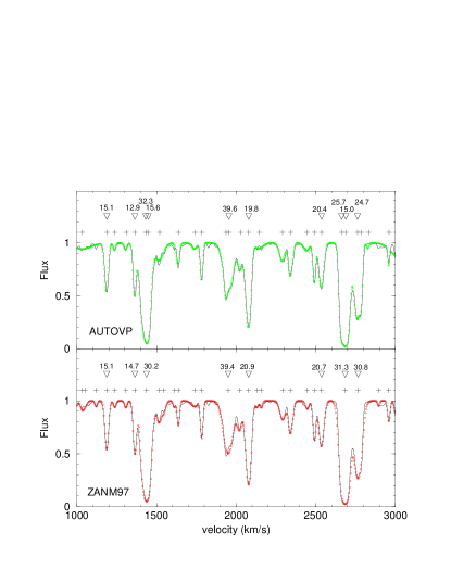
Figure 7: A comparison of the same simulated spectrum fit with two different techniques, one without noise ([Zhang et al. 1997], denoted ZANM97 in the figure) and one with noise (AUTOVP, kindly provided by Romeel Davé). The spectrum is from the $128^{3}$ simulation at $z=3$. The simulated spectrum is shown with a solid lines, while the fits are circles. Triangles indicate fit lines with column densities greater than $10^{13}$ cm^-2, and the associated numbers are the best fit $b$ parameters from each method. Notice that these larger lines are well reproduced and fit by both methods. Plus symbols give the locations of lines with all column densities found by the respective methods.

We fit one hundred of our $\Delta z=0.1$ spectra for a relatively difficult case, the $128^{3}$ simulation at $z=3$, which exhibits many narrow lines. The result, shown in Figure 8, demonstrates that while there are some differences — which would be greater for lower signal-to-noise spectra — the basic outcome is unchanged. Indeed, this is unsurprising: the presence of metal lines in observed spectra proves that there is no intrinsic difficulty in fitting thin lines. The median $b$ parameters of the two distributions differ by only 1.7 km/s (19.9 km/s for the method of ZANM97 compared to 18.2 km/s for AUTOVP). This difference reflects the fact that Voigt-profile fitting is not a highly robust way to fit these lines, but we argue it is sufficient to differentiate between the spectra predicted here and those observed.

Figure 8: A comparison of the Doppler $b$ distribution resulting from fitting with two different techniques, one without noise (ZANM97) and one with noise (AUTOVP). The spectra are from the $128^{3}$ simulation at $z=3$.

Another possibility that we can examine is the effect of changing the photo-ionization rate and hence the average flux decrement, which is not all that well determined observationally: ranging from 0.22 ([Zuo & Lu 1993]) to 0.36 ([Press et al. 1993]) at $z=3$. In the simulations, changing the value of $h$, $\Omega_{b}$ or the ionizing flux results in a rescaling of the optical depth. To a good approximation (particularly for the lower-column density lines) this simply has the effect of multiplying the column densities by a constant factor and shifting the distributions shown in Figure 4. This changes the number of lines observed in a given interval in $N_{HI}$, however, it has relatively little effect on the shape of the $b$-distribution or on its median value, which changes by only 1.5 km/s if we renormalize to a mean flux decrement of 0.36 (as opposed to values of around 0.22 without renormalization).

2.4 What causes $b$ to decline with resolution?

The width of a particular line can be affected by the gas temperature, the peculiar velocity structure, and the density profile of the line. An increase in the temperature would increase the Doppler broadening; an expanding structure (or even one collapsing less quickly) can broaden the profile; finally the density distribution itself can give rise to such an effect since a line that is physically wider will cover more of the Hubble flow.

In order to determine the cause of the decline seen in the previous section, we must look at the underlying gas distribution that gives rise to each line. In Figure 9 we plot the same line-of-sight for the three different resolutions at $z=3$. There is rough correspondence between large features, however the details vary strongly, particularly for the $32^{3}$ run (compared to the others). Unfortunately, a comparison of this type is not particularly useful due to the chaotic nature of the non-linear evolution; slight differences in, say, the position of a clump can give rise to large discrepancies along a particular line of sight. Still, a number of broad conclusions can be drawn. The first is that the large-scale velocity and density structures are well followed, although in at least one case (around 200 km/s), the differences are surprisingly large. The two better-resolved simulations tend to track each other with satisfying fidelity. The second is that a qualitatively new feature appears to have arisen in the high-resolution temperature profiles — high amplitude fluctuations on the 20 km/s (100 $h^{-1}$ kpc) scale. We will return to this observation below.

Figure 9: The profiles of various quantities resulting from the same line-of-sight taken through the three simulations at $z=3$. The ordinate is the Hubble velocity corresponding to that cell (for baryonic density, temperature, velocity, and HI density) or the wavelength (converted to km/s) for the flux.

While such anecdotal evidence is interesting, it is more useful to look at the mean behaviour of the lines. The difficulty in doing this is to associate a given flux decrement (line) with the range of cells which create it. Because of Doppler shifts due to peculiar velocities in the gas, there does not have to be a one-to-one correspondence. However, for the vast majority of lines, the correspondence is clear. Still, we need to remove the peculiar velocity contribution in order to do this association; fortunately, the bulk velocity component changes slowly, so this task is relatively straightforward.

Another way to state the problem is that given the center of a line, $v_{line}$, in the optical depth distribution $\tau(v_{line})$, how do we find the corresponding point $x$ in $\rho(x)$ or $T(x)$, where $x$ is the distance along the line of sight? The two are related through $v_{line}=H(z)x+v_{pec}(x)$, or more precisely, $\tau(v_{line})$ is given by an integral over $x$, which we write schematically as $\tau(v_{line})=\int(d\tau/dx)dx$ (for more details see [Zhang et al. 1998]). Since the $v_{line}$-$x$ relation cannot be directly inverted, the obvious approach is to solve it iteratively; however, this runs into convergence problems. Instead, we replace the term $v_{pec}(x)$ with:

$$\bar{v}_{pec}(v_{line})=\tau(v_{line})^{-1}\int{\frac{d\tau}{dx}v_{pec}(x)dx},$$ (2)

which is the (optical-depth weighted) mean peculiar velocity of the absorbing gas. This value is then used to correct the observed line-center to our estimate of the line-center as measured by the Hubble velocity along the line-of-sight: $v_{h}=H(z)x=v_{line}-\bar{v}_{pec}$.

We then follow the LOS in both directions (positive and negative velocity) until a density minimum is encountered in the baryon distribution along each path. The cells between these two density minima are extracted and used to compute the mean profiles shown in Figure 10 (in order to prevent small fluctuations from introducing small minima which would cause us to extract too small a section, we smooth the density slightly, but only while checking for minima). We discard lines that do not have a density maximum within 20 km/s of the estimated line center (about 5% of the total), since visual inspection of a sample of these showed them to fall on the wings of much larger lines. This entire procedure is robust to small changes in the details.

Figure 10: Mean profiles, at $z=3$ of (from top to bottom) baryon overdensity, dark matter overdensity, temperature, and peculiar velocity projected along the line of sight. The left column shows results from three simulations with varying resolution for lines with neutral hydrogen column densities in the ranges $N_{HI}=10^{13.0}-10^{13.1}$ cm^-2. In the upper left panel, three lines show the cell size for each simulation. The right column shows the same quantities from the highest resolution simulation for a range of column densities. From bottom (dotted) to top (solid), the lines correspond to column densities in the ranges: $N_{HI}=10^{12.0}-10^{12.1},10^{12.5}-10^{12.6},10^{13.0}-10^{13.1},10^{13.5}-10^{13.6}$ and $10^{14.5}-10^{14.7}$ cm^-2.

Since the column density is a robust prediction, we extract those lines which lie within a small range of $N_{HI}$ and plot the results in Figure 10. We first discuss the left hand column, which shows a resolution study for a large number of lines (drawn from 300 samples each of length $\Delta z=0.1$) from the same three simulations discussed previously. Only lines in the range $N_{HI}=10^{13.0}$–$10^{13.1}$ are used. Although individual lines can differ in detail, these mean profiles are characteristic; to give an idea of the variation, the rms scatter in $\rho_{b}/\left<\rho_{b}\right>$ is about 0.3. The dark matter, which is represented as particles rather than cells in the simulation, is interpolated to a mesh with the tri-linear cloud-in-cell method. We first address the effect of resolution, and then, in the next section, turn to what the figure can tell us more generally about the lines.

Systematic resolution effects are visible in each quantity. The density profiles, both baryonic and dark, are narrower with higher resolution, although the largest changes are in the dark matter profile, while the baryons show a flatter central profile. The temperature profile is relatively unchanged, although it becomes somewhat narrower and features a central depression at high resolution. The peculiar velocity profile develops a kink in the central 20 km/s with cell sizes less than 37.5 $h^{-1}$ kpc.

This figure confirms ([Weinberg et al. 1997]) that a significant part of the line-broadening — at least for low-column density lines — is due to the Hubble flow across the line width, although thermal Doppler broadening also makes an important contribution. These statements are made a little more precise in Figure 11, which converts the mean density and temperature profiles from Figure 10 into an optical depth, assuming ionization equilibrium. In this case the HI opacity is proportional to $\rho^{2}\alpha(T)\sim\rho^{2}T^{-0.7}$, where $\alpha(T)$ is the recombination coefficient.

Figure 11: This figure shows how Hubble broadening, peculiar velocities and thermal broadening affect the mean line profile for lines with $N_{HI}$ in the range $10^{13.0}-10^{13.1}$ cm^-2. The dashed line shows an estimate of the optical depth ($\rho^{2}T^{-0.7}$, from the $128^{3}$ simulation shown in Figure 10), the dotted line adds the distortion due to the mean peculiar velocity profile, and the solid line also includes thermal broadening. The dot-dash lines demonstrates that a Gaussian is a good fit to the resulting profile.

Without any peculiar velocities or thermal broadening, the resulting profile would be the dashed line. For such low optical depths, a Voigt profile is indistinguishable from a Gaussian. Although approximately Gaussian in shape, the profile shown here is not exactly so, and fits produce $b$ parameters ranging from 10 to 15 km/s, depending on which part of the curve is fit. The dotted line includes the mean peculiar velocity, which shifts the observed velocities of the profile ($v=v_{H}+v_{pec}$), and multiplies the optical depth by $(1+dv_{pec}/H(z)dx)^{-1}$. The boxy shape is a result of the kink in the velocity profile. Adding thermal broadening is enough to make the spectrum quite Gaussian, as the fit in the figure demonstrates. This is important, since it is this shape that is used to fit lines in the observed spectrum and suggests that Voigt-profile fitting, although often criticized, may be more robust than commonly assumed. Still, it must be kept in mind that in this exercise we have averaged the density, temperature and peculiar velocity separately and then formed a mean profile, which is quite different from averaging the optical depth distribution directly. Moreover, even if the average shape is Gaussian, individual lines may vary substantially.

Returning to Figure 10, we can now try to answer the question posed earlier. Of the three possible causes for the decrease in the line width, the most significant is the density, which shows a clear decrease in width as the resolution improves. This is particularly true in the outskirts of the line, which contributes preferentially to the line thickness. This can be roughly quantified by the width of a Gaussian fit to the density profile. Although it is approximately Gaussian in shape, it is impossible to fit both the inner and outer parts with the same parameters; however, using only the outer points (beyond $\pm$ 10 km/s), the fit width decreases by 25% in going from the $32^{3}$ to the $128^{3}$ simulation. The inner part shows a less dramatic 10% decline. These figures are comparable to the drop in the median $b$ with resolution.

This plot also shows that the change in the peculiar velocity is not primarily responsible for increasing the line width, since the magnitude of the change is only around 1 km/s. The temperature also adds to the width somewhat, as the high resolution profile is narrower, so the gas temperature in the line edges is reduced. This reduces the Doppler broadening (which contributes a width of approximately 13 $(T/10^{4}$K$)^{1/2}$ km/s), but again only by about 1 km/s or so.

From this discussion, we can conclude that the primary reason for the shift in the $b$ distribution is numerical thickening of the lines. This shows up most clearly in the density profile, but it also affects the temperature distribution.

2.5 The physical nature of the absorbers

These profiles also tell us a great deal about the physical nature of the absorbers. The velocity plot (still focusing on the left hand side of Figure 10) indicates that these lines are infalling in comoving coordinates, but the amplitude, which is less than the Hubble expansion, reveals that the objects are actually expanding in absolute coordinates. Thus, while the overdensity ($\rho_{b}/\left<\rho_{b}\right>$) may be increasing slowly, the absolute density is dropping (at least for absorbers with this column density).

The temperature follows largely from the density profile: the recombination rate is larger at higher densities and so photoionization heating is more effective. Lower densities have also undergone more expansion cooling. This dependence on density results in a polytropic equation of state ([Hui & Gnedin 1997]; see also [Giroux & Shapiro 1996]): $T\sim\rho^{0.4}$, by $z=3$. The temperature contributes a width to the lines via Doppler broadening which is approximately 13 $(T/10^{4}$K$)^{1/2}$ km/s, and so dominates the width only for lines which are intrinsically thin.

Finally, we turn to the details of the line center. The baryon density profile shows a rounded top as opposed to the cuspy center of the dark matter. This is due to the effect of thermal pressure. Prior to reionization, the gas and dark matter profiles follow each other; however, once reionization occurs the gas temperature is raised everywhere to a nearly constant 15,000 K (the exact temperature depends somewhat on the assumed ionizing spectrum). The gas in the center of these objects, which are most likely to be sheets or filaments (e.g. [Zhang et al. 1998]), finds itself over-pressured and starts to expand. This (relative) expansion can be seen in the peculiar velocity profile as the kink mentioned previously, and also cools the gas, causing the central temperature depression.

To see that the pressure gradient is sufficient to accomplish this, we note that the acceleration from the pressure $p$ is $\nabla p/\rho\approx c_{s}^{2}\nabla\rho/\gamma\rho$, where $c_{s}$ is the sound speed and the second step uses the fact that the temperature is nearly constant at recombination. Approximating the gradient $\nabla\rho$ as $\Delta\rho/\Delta r=\Delta\rho H(z)/\Delta v$, we can write the velocity change after a Hubble time as $\Delta v=c_{s}(\Delta\rho/\gamma\rho)^{1/2}$. Since the sound speed is about 10 km/s at $10^{4}$ K, and the gradient term is of order unity or higher, it’s clear that a velocity change of the required magnitude can be generated as long as the initial peculiar velocities are not too large.

On the right-hand side of Figure 10 are plotted mean profiles for a range of column densities from $N_{HI}=10^{12}$ to $10^{14.5}$ cm^-2 (now using only the highest resolution simulation). Above this value there are too few lines, with too much diversity for a reasonable mean profile to be constructed. Other studies ([Zhang et al. 1998]; [Cen & Simcoe 1997]) have shown that the highest density absorbers ( $N_{HI}\ga 10^{14}$ at $z=3$ in this model) tend to be quasi-spherical, lying at the intersection of filaments, while progressively lower density absorbers occur in filaments and then sheets. We focus mostly on low column-density lines and so on these latter two kinds of absorbers. We remind the reader that this correspondence between overdensity and column density depends not only on redshift, but also on a number of model-dependent factors, including $\Omega_{b}$, $h$ and the photo-ionization rate. For example, lines with column densities of $10^{14}$ cm^-2 are associated with mean overdensities of 3-4 in these simulations, but 1-2 in those of Davé et al. (1998b)dav98b, primarily due to their renormalization to a higher flux decrement.

The density profiles, particularly for the dark matter, are remarkably similar in shape, showing little variation in width and are simply scaled in amplitude. The gas distribution becomes more and more peaked for lines with larger $N_{HI}$, as the thermal pressure that gives rise to the rounded distribution for low-column density lines becomes less important (see also [Meiksin 1994]). This can be quantified by comparing the FWHM of the dark matter and gas profiles, as is done in Table 2.5. The ratio varies from 3:1 at low column densities, to nearly equal by $N_{HI}=10^{14.5}$ cm^-2.

cccccc Relative contributions from Hubble and thermal broadening to lines of various column densities 0pt & $N_{HI}=10^{12.0}$ $N_{HI}=10^{12.5}$ $N_{HI}=10^{13.0}$ $N_{HI}=10^{13.5}$ $N_{HI}=10^{14.5}$ peak overdensity & 0.28 0.51 1.1 2.7 13 0.46FWHM_dm 4.9 4.2 4.2 4.1 4.8 0.46FWHM_gas 14.8 12.4 10.6 7.5 5.2 $b_{T}$ (thermal) 9.7 10.5 12.4 16.8 23.3 $\sqrt{(\hbox{0.46FHWM${}_{gas}$)}^{2}+b_{T}^{2}}$ 17.7 16.2 16.3 18.4 23.9 median $b$ from fits 14.9 15.6 18.0 20.1 22.6

We can also use this information to obtain a rough estimate of the relative contributions of Hubble and thermal broadening. Since the optical depth is given by $\tau\sim\rho^{2}T^{-0.7}$ and $T\sim\rho^{0.4}$ (see Figure 3 and [Hui & Gnedin 1997]), we can write $\tau\sim\rho^{1.7}$. If the density distribution were a Gaussian, then the optical depth profile would also be a Gaussian, with $b=$FWHM$/(2\sqrt{1.7\ln 2})\approx 0.46$ FHWM. In Table 2.5 we give this value, which is roughly the contribution from Hubble broadening to the total width of the line. We also include the $b$ parameter that would result from thermal broadening alone, using the mean temperature of the profile (weighted by $\rho^{2}T^{-0.7}$). In the second last row, these two values are added in quadrature. The result is broadly consistent with the median $b$ derived from fitting Voigt profiles to the spectra, which is shown in the final row. The difference is most likely because 0.46FWHM is an underestimate of the effect of Hubble broadening, and it should be kept in mind that we are ignoring the effect of peculiar velocities. Note in particular that as the Hubble width of the lines decrease with increasing column density, the temperature grows, leaving the resulting width more-or-less constant. This is consistent with the lack of a strong correlation between $N_{HI}$ and $b$ in the simulations, and helps to explain why the median of the $b$ distribution is insensitive to the normalization of the mean decrement.

The central temperature dip and the velocity kink become less pronounced with increasing column density up until $N_{HI}\sim 10^{14}$. At this point, the peculiar infall velocity actually becomes larger than the Hubble flow and the object has detached from the Hubble expansion and is collapsing. Once this happens, two shocks form on either side of the mid-plane and propagate outwards (visible in the velocity distribution at $\pm 10$ km/s). If this occurs in a sheet, then the object forms a Zel’dovich pancake (otherwise the shock is cylindrical in the case of a filament or quasi-spherical for a knot). These lines are now dominated by thermal broadening, since $v_{pec}\sim-v_{hub}$. It is interesting to note that this qualitative change in the physical nature of the line occurs at $N_{HI}\sim 10^{14.5}$ cm^-2, which is also where it appears that the carbon abundance (and by plausible extension, all metals) undergoes a drastic change: from [C/H] $\sim-2.0$ above this cutoff, to less than -3.5 below ([Lu et al. 1998]). Similar results have been found using OVI as a probe ([Davé et al. 1998]). This behaviour is in broad agreement with that predicted in the simulations of Gnedin & Ostriker (1997)gne_ost97, which explicitly include star formation and the production of metals.

Finally, we comment on the fact that the density away from the line drops below the cosmic mean, and in fact, the central values of the smallest lines are consistently below this value. This means that most low column density lines are in voids. The size of these regions are smaller than familiar galactic voids and so the name mini-void has been proposed ([Zhang et al. 1998]).

2.6 Resolving the Jeans length: reionization-driven winds

The thermal pressure becomes more important for smaller lines until it is sufficient to disperse the feature entirely ([Bond, Szalay & Silk 1988]). As we pointed out earlier, the highest resolution simulations show small scale fluctuations in the velocity and temperature distributions that are mostly absent in the lower resolution runs. Here, we offer an explanation for that behaviour. In Figures 12, 13, and 14, we plot the baryon and dark matter density, the temperature and the projected peculiar velocity along a line-of-sight of constant comoving length at redshifts from $z=7$ to $z=2$.

Figure 12: The evolution of the baryon (solid) and dark matter (dashed) overdensities ($\rho/\left<\rho\right>$) along a line of sight for the highest resolution simulation ($128^{3}$ cells). The ordinate is the Hubble velocity at $z=2$, with the other redshift ranges adjusted to cover the same comoving length.

Figure 13: The evolution of the baryon temperature along the same line of sight shown in Figure 12.

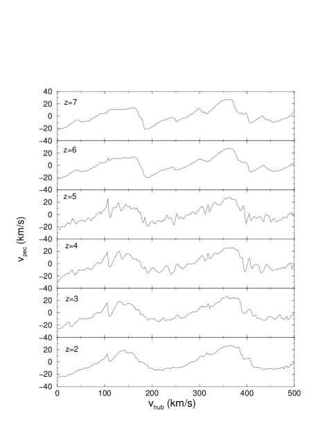
Figure 14: The evolution of the projected baryon peculiar velocity along the same line of sight shown in Figure 12.

At the earliest time, many of the smallest clumps (which are not fully resolved even at this resolution) have collapsed into sharp density spikes, and the baryons follow the dark matter distribution quite well. In this model, re-ionization occurs shortly after $z=7$ and by $z=6$, the gas is almost all uniformly at $T=15,000$ K, regardless of density. The thermal pressure is then proportional to the density (since $p\propto\rho T$) and the clumps, filaments and sheets which are not sufficiently massive to generate a gravitational force larger than this thermal one begin to expand. Roughly, this constraint can be expressed as the requirement that an object must be larger than the Jeans length: $\Delta v_{j}=H(z)r_{j}=26.3$ $(T/10^{4}K)^{1/2}$ km/s.

After re-ionization, the smallest objects expand, driving out a wind. The result can be seen in the density field, as a smoothing of the smallest scales, but it is in the temperature and velocity fields where the changes are the most startling. By $z=5$, these winds produce small-scale fluctuations in the velocity, and in the temperature, as the resulting expansions and contractions cause adiabatic cooling and heating. The fluctuations decay at late times, as the gas rearranges itself to new equilibrium configurations.

We argued in section 2.5 that this process can accelerate gas to velocities around the sound speed for the lowest column density lines, so for these objects – which are smaller – the gas velocities should be slightly lower. Indeed, Figure 14 shows fluctuations of around 5 km/s. For an adiabatic gas with a ratio of specific heats $\gamma$, the temperature change will be $\Delta T/T=(\gamma-1)\Delta\rho/\rho$. From Figure 12, we see that $\Delta\rho/\rho$ can approach unity, so large changes in the temperature are expected provided that the timescale for radiative processes is longer than the dynamical time (i.e. the gas is adiabatic). The dominant heating mechanism is photo-ionization heating, which is limited by the recombination time-scale: $t_{R}=2.3\times 10^{17}(T/10^{4}K)^{0.7}((1+z)/4)^{-3}(\rho/\bar{\rho})^{-1}$ s, while a 5 km/s wind can cross two cells (approximately our resolution limit) in $5.8\times 10^{16}((1+z)/4)^{-1}$ s.

It is these winds, driven by reionization, that produce the scatter in Figure 3, as the resolution improves. In detail, the process of dispersing sub-Jeans length clouds is not modeled correctly, partially because we do not have the necessary resolution, but also because we have approximated the radiation field as uniform and isotropic. In fact, discrete ionizing sources will produce I-fronts, which will drive a rocket effect, accelerating the cloud in the direction of the radiation, until it is completely ionized and disperses ([Shapiro, Raga & Mellema 1998]). Still, the net result should be grossly similar unless an object is sufficiently dense that it is optically thick to the ionizing radiation. Such clouds, in order to survive, will have high column densities ($N_{HI}>10^{18}$) and have been proposed as the source of some Lyman-limit systems ([Abel & Mo 1998]). However, unless a significant fraction of the mass is tied up in such systems, they will not greatly affect our results.

2.7 Other statistical measures

The objects that give rise to absorption features in the Ly$\alpha$ forest are generally not the thermally broadened, compact clouds that the Voigt profile assumes (although it is interesting to note that their mean shape is not so different from a Gaussian). Since this profile is not always a good fit to the observed (or simulated) features, it makes sense to develop other, less parametric ways to characterize the observations. Perhaps the most straightforward is to work directly with the N-point distribution functions of the transmitted flux ($F=e^{-\tau_{HI}}$) itself ([Miralda-Escudé et al. 1997]; [Rauch et al. 1997]; [Cen 1997]).

In Figure 15, we show the probability distribution at $z=3$ from 300 lines-of-sight through the same three simulations previously discussed. The photoionizing flux has been rescaled so that the mean flux decrement ($D_{A}=1-F$) is 0.36 ([Press et al. 1993]). The two higher-resolution results show very similar distributions, while the lowest exhibits a deficit around $F\sim 0.95$ and a corresponding surplus near $F\sim 0.8$. This follows simply from the profile broadening noticed earlier: narrow lines dip down deeper and so produce lower values of the transmitted flux (higher decrements), leaving more of the spectrum near its continuum value.

This redistribution of the flux will obviously affect zero-point statistics such as the mean decrement. For example, without renormalizing, the average decrement decreases with resolution: $D_{A}=0.229,0.217,0.214$ for the $32^{3}$, $64^{3}$ and $128^{3}$ simulations, respectively. While this is relatively slight, the effect on the He will be greater (see also [Zhang et al. 1998]).

Figure 15: The probability distribution (top) of the transmitted flux at $z=3$ for the same three simulations with different resolutions shown in Figure 4. The bottom panel plots the mean flux difference as a function of velocity difference for pixels in the ranges indicated (eq. 3).

A higher order statistic than the flux distribution is the two-point function $P_{2}(F_{1},F_{2},\Delta v)$, which gives the probability that two pixels with separation $\Delta v$ will have flux $F_{1}$ and $F_{2}$. In order to present this function graphically, we plot normalized moments of it, averaged over a range of flux ($F_{a}$ to $F_{b}$):

$${{\int_{F_{a}}^{F_{b}}dF_{1}\int_{0}^{1}dF_{2}P_{2}(F_{1},F_{2},\Delta v)(F_{1}-F_{2})}\over{\int_{F_{a}}^{F_{b}}dF_{1}\int_{0}^{1}dF_{2}P_{2}(F_{1},F_{2},\Delta v)}}$$ (3)

This is the average flux difference as a function of velocity for pixels in the range $F_{a}$ to $F_{b}$, and is plotted in the bottom panel of Figure 15 for three ranges. Although somewhat complicated, it can be interpreted in the following way. For small separations, there is little difference regardless of the flux value, or in other words there is high coherence for small $\Delta v$, a fact which is clear from just looking at the spectra. At large separations ($\Delta v>200$ km/s), there is no coherence, and the value is just the difference between the mean value of the transmitted flux (0.65) and the mean flux in the interval $F_{a}$ to $F_{b}$. For intermediate separations, in the range $\Delta v=10$ to 100 km/s, the plot shows a measure of the mean profile around pixels with fluxes in that interval (this is heavily influenced by the structure of lines, but around 100 km/s line-line correlations also play a role).

The effect of resolution is again clear, narrowing the line profile as the cell size decreases. Therefore we see that this effect shows up not just in the parametric analysis (Voigt-fitting), but in the distribution of fluxes as well. Although the difference looks smaller in this plot, that is largely a function of the compressed scale. For example, if we take the $0<F<0.1$ profiles and ask at what $\Delta v$ do the lines go through a mean flux difference of 0.3 (which is an approximate measure of the line width), the answer is 43 km/s for the $32^{3}$ simulation, but only 35 km/s for the $128^{3}$ run. While the absolute numbers differ, this records a drop in width of nearly 19%, comparable to the decline in the median $b$ parameter.

2.8 The effect of large-scale power

In this section, we study the effect of additional large-scale power (see also [Wadsley & Bond 1997]), to address the question: are the results of the previous discussion biased by the small box size?

In Figure 16, we show density and (volume-weighted) temperature distributions for four simulations with increasing amounts of large-scale power but the same resolution. The smallest box is the same $32^{3}$ simulation analyzed above, while the largest is a $256^{3}$ simulation with a 9.6$h^{-1}$ Mpc box size. The distributions are remarkably similar, although there are some differences, particularly for the two smallest boxes.

Figure 16: The distribution of baryon overdensity (top) and volume-weighted temperature (bottom) for four simulations with increasing box size — but the same resolution — at $z=3$.

The biggest difference due solely to the presence of long-wavelength modes is the increased amount of high-temperature gas. As larger modes are included, the bulk velocities increase and the gas that is shock-heated around the edge of the biggest sheets, filaments and knots is correspondingly hotter. If we were looking at the formation of very dense, and hence very rare, clumps (galaxies and groups), we would also see an increase in the number of these objects; however, their absence has little effect on the low-density regions that occupy most of the volume and hence on the Ly$\alpha$ forest itself. The scatter at high density for the small boxes is simply due to Poisson fluctuations since they have much smaller samples.

The other difference that is apparent is a small shift in the peak temperature, and a slight rearrangement in the low-density end of the baryon distribution (particularly evident in the low $\rho_{b}$ tail). The evolution of the small boxes is mostly guided by the largest modes in the box, which are not well sampled (i.e. are determined by a small number of random values). They become quasi-linear by $z\sim 3$ and mode-mode coupling starts to play a role, spreading their influence over a wide range of scales. Also, there are no fluctuations above the box size so mode-mode coupling cannot transfer that power down to smaller scales. This means that, on average, there tends to be a deficit of power in small boxes.

Put more simply, these boxes are not fair samples, In, fact, if the smaller box sizes (1.2$h^{-1}$ and 2.4$h^{-1}$ Mpc) are repeated with a different initial random seed, they show variations of the same magnitude. However, the two larger volumes show nearly identical distributions.

Figure 17: The distribution of neutral hydrogen column densities for the same simulations shown in Figure 16, at three different redshifts.

Turning to the observable quantities, we show in Figure 17 the distribution of column densities for these same four simulations, demonstrating again the robustness of this measure. There are, however, some systematic differences, notably for the smallest box which shows a distinct overproduction of moderate to high column density lines. This is again due to the fact that we are not simulating an adequately large volume to contain a reasonable sample, a situation which gets worse at lower redshift as larger regions go non-linear. Although in this case, the result is a flattening of the power-law distribution, we argue that in general either case could occur depending on whether the fluctuations are systematically larger or smaller than average. If we fit power laws to these distributions, the slopes differ by less than 2% for the two largest boxes, but show variations of twice that value for the smaller volumes.

Figure 18: The distribution of Doppler $b$-parameters for the same simulations shown in Figure 16, at three different redshifts.

The same effect is operating in the distribution of Doppler $b$ parameters, plotted in Figure 18, causing shifts in the entire distribution for the smaller boxes, while the larger boxes show nearly identical distributions. The magnitude is about 2.5 km/s at $z=3$.

This is consistent with the fact that scales which give rise to fluctuations on the few hundred kpc scale require box sizes of around 5 $h^{-1}$ Mpc to resolve properly. For example, the measure of small scale fluctuations suggested by Gnedin (1998)gne97:

$$\sigma^{2}_{34}=\int_{0}^{\infty}P(k)e^{-2k^{2}/k^{2}_{34}}{{k^{2}dk}\over{2\pi^{2}}}$$ (4)

(where $k=2\pi/L$, $P(k)$ is the power spectrum at $z=3$ and $k_{34}=34\Omega_{0}^{1/2}h$ Mpc^-1) can be used to make this argument more concrete. If, instead of integrating from 0, we use $k=L/2\pi$ with $L$ the size of the box, and denote this quantity $\sigma^{2}_{34}(L)$, then the ratio of the power included within the box to the total power: $\sigma^{2}_{34}(L)/\sigma^{2}_{34}=0.67/0.82/0.92/0.96$ for $L=1.2/2.4/4.8/9.6$ $h^{-1}$ Mpc.

3 Discussion

In the previous section we have shown that while the column density distribution is not a sensitive function of resolution, the Doppler $b$ distribution is: systematically shifting towards lower $b$ with increasing resolution. This is important because the median of this distribution was already marginally low for this model, compared to observations. We demonstrated that this decrease is due to intrinsic changes in the density profile, rather than the temperature or the velocity structure of the lines. The small volumes used to obtain high resolution do cause some change in the median $b$, but not enough to explain the discrepancy with observations. In this section, we turn first to modeling the effect of resolution, shedding some light on the shape of the $b$-distribution. Then we briefly discuss ways to reconcile our result with observations.

3.1 Modeling the $b$-distribution

One of the traditional difficulties in understanding this distribution is the presence of large $b$ values (e.g. [Press & Rybicki 1993]). To be explained by Doppler broadening, these systems require temperatures too large to be explained by thermal equilibrium. The simulations also produce a large tail, and yet for large $b$ lines with a given column density, we do not see a correlation between the width of a line and the temperature of the underlying gas. It has recently been pointed out that such a tail is a natural consequence of the filamentary and sheet-like nature of CDM-like structure formation ([Rutledge 1998]), and the high-$b$ lines arise from oblique lines-of-sight through these structures. To test this idea, we compute, for a large sample of lines, the alignment between the density gradient and the line-of-sight vector:

$$\cos\left(\theta\right)=\sum{{{|\bf\nabla}\rho_{b}\cdot{\bf x}|}\over{|{\bf\nabla}\rho_{b}|}}.$$ (5)

The sum is over cells that give rise to the line and ${\bf x}$ is the line-of-sight unit vector. For sight lines which go perpendicularly through a sheet or filament, the two vectors should line up perfectly and $\cos(\theta)=1$, while the measure goes to zero as ${\bf x}$ becomes parallel to the filament. Figure 19 shows that while there is a lot of noise in the relation, the correlation is clear and goes in the expected direction.

Figure 19: The mean alignment of the density gradient and the line-of-sight vector ($\cos(\theta)$) decreases with $b$. In order to give an idea of the scatter, the error bars show the standard deviation for each bin.

This picture of the clouds also gives us insight into the effect of resolution. It has proved useful to model this effect in Eulerian simulations as a Gaussian smoothing of the density field, with a kernel of approximately two cells ([Bryan & Norman 1998]). Such a convolution means that the width of a given structure — whether sheet, filament or sphere — would be increased by adding the intrinsic width of the structure and the size of the smoothing kernal in quadrature: $l^{\prime}=\sqrt{l^{2}+(2\Delta x/(1+z))^{2}}$, where $l$ is a measure of the structure’s intrinsic width in proper coordinates, $\Delta x$ is the comoving cell size and $l^{\prime}$ is the resolution-thickened width.

If we now return to our model for the formation of the lines and make two simplifying assumptions: (1) that all lines are due to the oblique passage of a line-of-sight through filaments or sheets which all have width $l$, and (2) that Hubble broadening dominates, we can construct a method for correcting for this convolution. Together these assumptions imply that the width of a line is given by $b=H(z)l\cos(\theta)$ and that the variation in $b$ is due to variation in $\theta$, the angle between the line-of-sight and the normal of the filament or sheet. This means that the ratio of the numerically thickened line width to its intrinsic width is given by:

$$f(\Delta x)=\frac{b^{\prime}}{b}=\left(1+\left(\frac{2\Delta x}{l(1+z)}\right)^{2}\right)^{1/2}$$ (6)

Notice that this expression does not depend on $b$, so it is a constant for all lines (given our assumptions). Unfortunately, we don’t know $l$; however, if we can associate $l$ with the width of the median, $b_{m}$, then $l=b_{m}/H(z)=b^{\prime}_{m}f(\Delta x)/H(z)$ and the correction factor $f(\Delta x)$ can be expressed directly in terms of measurable quantities:

$$f(\Delta x)=\left(1-\left(\frac{2\Delta xH(z)}{b_{m}^{\prime}(1+z)}\right)^{2}\right)^{-1/2}.$$ (7)

This provides a method to correct the measured $b$-parameter of a given line which depends only on the measured median of the (numerically thickened) distribution and $\Delta x$, the comoving cell size (as well as some cosmological factors): we simply replace the measured $b^{\prime}$ with $b=b^{\prime}/f(\Delta x)$. Of course, given our simplistic assumptions, it is unrealistic to expect this to work on a line-by-line basis, but there is some hope it may provide a good statistical correction. We expect it to be least accurate for lines arising from spherical absorbers, which tend to be higher column density lines anyway, and for which our assumption of Hubble broadening also probably fails. This is one reason we restrict our range of $b$ parameters to the lower column density end ($N_{HI}=10^{13}-10^{14}$ cm^-2). It will also be less accurate for those lines which have small values of $b$ and are probably dominated by variation in $l$ rather than $\theta$.

We test the correction on the distributions plotted originally in Figure 5. Since they are log-log plots, we can simply shift the curves to the left (and up, since the distribution is per unit $b$) by the constant factor $\log{f(\Delta x)}$. The result is shown in Figure 20.

Figure 20: The distribution of Doppler $b$ parameters (for lines with column densities $10^{13}<N_{HI}<10^{14}$ cm^-2) for the same three redshifts and resolutions as in figure 4 (the box size is 1.2$h^{-1}$ Mpc). The distributions have been scaled to account for resolution as described in the text.

This scaling works remarkably well, except for the low $b$ end of the distribution at $z=4$ (and to a lesser extent at $z=3$). This is not surprising, given that our approximation breaks down for low $b$ values. Still, it provides a useful way to correct lower resolution simulations: distributions can be scaled as described above and the median (or mean) corrected by equation 7. For example, the median values predicted at $z=2$ are 21.0, 21.3, 21.4 km/s for the the $32^{3}$, $64^{3}$ and $128^{3}$ simulations. For $z=3$ these numbers are 19.8, 19.7 and 19.5 km/s, while for the worst case, $z=4$, they are 18.1, 18.9 and 17.5 km/s.

The ability to do this correction is important since it is difficult to perform a simulation which is both large enough and of sufficient resolution to reliably calculate the distribution. We make a best estimate for the median of the $b$ distribution in the range $N_{HI}=10^{13}$-$10^{14}$ cm^-2 using two simulations: one (L9.6 from Table 1), our largest simulation, but at a relatively low resolution, and another (L4.8HR) with better resolution, but a somewhat smaller box. The results are shown in Table 3.1, along with the uncorrected values.

cccc Best Estimate Median $b$-parameter 0pt simulation & $z=2$ $z=3$ $z=4$ L9.6 (corrected) & 24.8 22.3 25.8 L4.8HR (corrected) 22.7 19.2 20.4 L9.6 (uncorrected) 28.0 26.9 30.8 L4.8HR (uncorrected) 23.6 20.7 22.1

3.2 The conflict with observations

To highlight the fact that the predictions of this model for the $b$-parameter do disagree with observations, we plot both in Figure 21, for $z\sim 2$ and $z\sim 3$. While the shapes are roughly in agreement, the predicted medians are substantially too low, in both cases (the observed median is about 30 km/s). In this same plot, we also show the analytic profile suggested by Hui & Rutledge (1998)hui98, based on the Gaussian nature of the underlying density and velocity fields:

$$\frac{dN}{db}\propto\frac{b_{\sigma}^{4}}{b^{5}}\exp{\left[-\frac{b_{\sigma}^{4}}{b^{4}}\right]}.$$ (8)

The normalization and the parameter $b_{\sigma}$ have been adjusted to fit the simulations (observations) in the top (bottom) panel, in order to demonstrate the relatively good agreement in shape.

We remind the reader that our analysis technique is not the same as that used by observers, so we can not definitively rule out the possibility that this discrepancy is due to our difference in fitting Voigt-profiles to the spectrum (although we point out that Theuns et al. (1998) find a similar discrepancy with yet another analysis technique which is even closer to that used by the observers). Still, we have carried out a number of tests (see section 2.3) which indicate that it is relatively easy to measure the line width in our chosen column density range and that a bias of the required magnitude would be difficult to arrange. Probably the best way to confirm this result would be a non-parametric test dealing directly with the measured flux (as in section 2.7). An early indication of which way this will go can be seen by comparing our Figure 15 with its observationally determined counterpart in Figure 3 of Miralda-Escudé et al. (1997). By determining where the $0<F<0.1$ curves go through a mean flux difference of 0.3 in the respective plots, we can obtain a rough idea of the difference in the widths: for the observations, this is $\Delta v\approx 55$ km/s as compared to 35 km/s for our highest resolution simulation.

Previous work on the Ly$\alpha$ forest has, more often than not, stressed that the models were consistent with observations. In fact, this can be understood in terms of the analysis presented here. Other simulations of the SCDM model (ZANM97) found that the $b$-distribution matched well, however they only compared the results for their relatively low-resolution top grid (see Table 1) which, as we have shown, overestimates the resulting $b$-parameters. Similarly, we would argue that the SPH simulations of this model ([Hernquist et al. 1996]; [Davé et al. 1997]) predicted $b$-values that were somewhat too large (a conjecture confirmed by [Theuns et al. 1998]). Finally, turning to the last two entries in Table 1, the work of Miralda-Escudé et al. (1997)mcor had sufficient resolution to produce accurate $b$-values, and indeed their Figure 17b shows a $b$-distribution which certainly appears to have a median below that observed. However, the cosmological model is substantially different so a direct comparison is difficult.

Figure 21: The distribution of $b$ parameters for lines with column densities $10^{13}<N_{HI}<10^{14}$ cm^-2. The top panel shows observational data ([Kim et al. 1997]) at a mean redshift of 2.31 as well as the $b$ distribution from our $128^{3}$ simulation at $z=2$; The dashed line is an analytic profile fit to the simulated data. The bottom panel shows the profile for observational data at $z=3.35$ and simulated data from $z=3$. The same analytic profile is now fit to the observations.

How can we restore agreement?

One possible answer is to find a way to increase the temperature of the gas. While this will help by adding to the thermal broadening, it is clear that this will not be sufficient for the large $b$ lines. Another way to see this is, if thermal broadening dominated, then our calculations would predict a correlation between $b$ and $N_{HI}$ since there is a correlation between $T$ and $N_{HI}$; none is seen. Instead, the increased thermal pressure must act to widen the physical structures which give rise to the lines (this also means that we cannot mimic the effect in the simulations by simply increasing the temperature at the analysis stage). Figure 10 shows that such a process will require high temperatures, particularly for the larger column density lines.

Such a large increase (at least a factor of two) in the temperature seems to be difficult to accomplish. One way is to ionize He around $z\sim 3$, but this only appears to boost the temperature by at most 20% ([Hui & Gnedin 1997]; [Haehnelt & Steinmetz 1997]). Delaying reionization also helps because the gas retains some memory of its initial temperature, but even runs with sudden reionization at $z=5$ don’t change the $b$ distribution significantly. Similarly, increasing $\Omega_{b}$ boosts the equilibrium temperature, but because $T\sim\Omega_{b}^{1/1.7}$, even a factor of two change in $\Omega_{b}$ — which conflicts with big-bang nucleosynthesis — only increases the temperature by 50%, which is probably not enough. All runs in this paper have included a non-equilibrium chemical model, which increases the temperature slightly over the assumption of equilibrium ionization, but clearly not enough. We have, however, assumed that the radiation field is uniform. This approximation will modify the thermal history somewhat, but seems unlikely to have a large effect ([Meiksin 1994]; [Miralda-Escudé & Rees 1994]; [Giroux & Shapiro 1996]).

One last way to increase the gas temperature is to use thermal energy from star formation which, of course, we do not include in the simulations. This is difficult to rule out, but would require a remarkably high stellar energy input and the low metallicity of the low column density gas seems to argue against it ([Davé et al. 1998]; [Giroux & Shapiro 1996]).

Another way is to change the density distribution directly, through the power spectrum or cosmology ([Hui & Rutledge 1998]). We have only examined the standard cold dark matter model, and it is possible that other models will be more successful. We will address this topic in a future paper.

This work is done under the auspices of the Grand Challenge Cosmology Consortium and supported in part by NSF grants ASC-9318185 and NASA Astrophysics Theory Program grant NAG5-3923. We thank Tom Abel for the use of his rate coefficients, as well as Avery Meiksin and Jeremiah Ostriker for helpful comments. MLN acknowledges useful conversations with Martin Haehnelt. We thank the referee, David Weinberg, for many helpful suggestions that improved the quality of this work.

References

- [Abel et al. 1997] Abel, T., Anninos, P., Zhang, Y., Norman, M.L., 1997, New Astronomy, 2, 181
- [Abel & Mo 1998] Abel, T. & Mo, H.J. 1998, ApJ, 494, L151
- [Anninos et al. 1997] Anninos, P., Zhang Y., Abel, T., Norman, M.L., 1997, New Astronomy, 2, 209
- [Bi 1993] Bi, H.G. 1993, ApJ, 405, 479
- [Bi & Davidsen 1997] Bi, H.G. & Davidsen, A. 1997, ApJ, 479, 523
- [Bond, Szalay & Silk 1988] Bond, J.R., Szalay, A.S. & Silk, J. 1988, ApJ, 324, 627
- [Bond & Wadsley 1997] Bond, J.R. & Wadsley, J.W. 1997, to appear in Proceedings of the 13th IAP Colloquium, Structure and Evolution of the Intergalactic Medium from QSO Absorption Line Systems, eds. P. Petijean & S. Charlot (Nouvelles Frontières: Paris)
- [Bryan et al. 1995] Bryan, G.L., Norman, M.L., Stone, J.M., Cen, R., Ostriker, J.P. 1995, Comput. Phys. Comm., 89, 149
- [Bryan & Norman 1998] Bryan, G.L. & Norman, M.L. 1998, ApJ, 495, 80
- [Cen et al. 1994] Cen, R., Miralda-Escudé, J., Ostriker, J.P., Rauch, M. 1994, ApJ, 437, L9
- [Cen 1997] Cen, R. 1997, ApJ, 479, L85
- [Cen & Simcoe 1997] Cen, R. & Simcoe, R.A. 1997, ApJ, 483, 8
- [Croft et al. 1998] Croft, R.A.C., Weinberg, D.H., Katz, N., Hernquist, L. 1998, ApJ, 495, 44
- [Davé et al. 1997] Davé, R., Hernquist, L., Weinberg, D.H. Katz, N. 1997, ApJ, 477, 21
- [Davé et al. 1998] Davé, R., Hellsten, U., Hernquist, L. Katz, N. & Weinberg, D.H. 1998, ApJ, submitted (astro-ph/9803257)
- [Davé et al. 1998b] Davé, R., Hernquist, L. Katz, N. & Weinberg, D.H. 1998, ApJ, submitted (astro-ph/9807177)
- [Giroux & Shapiro 1996] Giroux, M.L. & Shapiro, P.R. 1996, ApJS, 102, 191
- [Gnedin 1998] Gnedin, N.Y. 1998, MNRAS, submitted (astro-ph/9706286)
- [Gnedin & Hui 1998] Gnedin, N.Y. & Hui, L.. 1998, MNRAS, 296, 44
- [Gnedin & Ostriker 1997] Gnedin, N.Y. & Ostriker, J.P. 1997, ApJ486, 581
- [Haehnelt & Steinmetz 1997] Haehnelt, M.G. & Steinmetz, M. 1997, MNRAS, submitted (astro-ph/9706296).
- [Haardt & Madau 1996] Haardt, F. & Madau, P. 1996, ApJ, 461, 20
- [Hernquist et al. 1996] Hernquist, L., Katz, N., Weinberg, D.H., Miralda-Escudé, J. 1996, ApJ, 457, 51L
- [Hu et al. 1995] Hu, E., Kim, T.-S., Cowie, L.L., Songaila, A., & Rauch, M. 1995, AJ, 110, 1526
- [Hui, Gnedin & Zhang 1997] Hui, L., Gnedin, N.Y. & Zhang, Y. 1997, ApJ, 486, 599
- [Hui & Gnedin 1997] Hui, L. & Gnedin, N.Y. 1997, MNRAS, 292, 27
- [Hui & Rutledge 1998] Hui, L. & Rutledge, R.E. 1998, preprint (astro-ph/9709100)
- [Kim et al. 1997] Kim, T.-S., Hu, E.M., Cowie, L.L. & Songaila, A. 1997, AJ, 114, 1
- [Kirkman & Tytler 1997] Kirkman, D. & Tytler, D. 1997, ApJ, 484, 672
- [Lu et al. 1998] Lu, L. Sargent, W.L.W., Barlow, T.A. & Rauch, M. 1998, preprint (astro-ph/9802189).
- [Machacek et al. 1998] Machacek et al. 1998, in preparation
- [McGill 1990] McGill, C. 1990, MNRAS, 242, 544
- [Meiksin 1994] Meiksin, A. 1994, ApJ, 431, 109
- [Meiksin & Madau 1993] Meiksin, A. & Madau, P. 1993, ApJ412, 34
- [Miralda-Escudé & Rees 1994] Miralda-Escudé, J. & Rees, M.J. 1994, MNRAS, 266, 343