The disruption of globular star clusters in the galaxy:
A comparative analysis between Fokker-Planck and $N$-body models.

Abstract

Recent $N$-body simulations have shown that there is a serious discrepancy between the results of the $N$-body simulations and the results of Fokker-Planck simulations for the evolution of globular and rich open clusters under the influence of the galactic tidal field. In some cases, the lifetime obtained by Fokker-Planck calculations is more than an order of magnitude smaller than those by $N$-body simulations. In this letter we show that the principal cause for this discrepancy is an over-simplified treatment of the tidal field used in previous Fokker-Planck simulations. We performed new Fokker-Planck calculations using a more appropriate implementation of the boundary condition of the tidal field. The implementation is only possible with anisotropic Fokker-Planck models, while all previous Fokker-Planck calculations rely on the assumption of isotropy. Our new Fokker-Planck results agree well with $N$-body results. Comparison of the two types of simulations gives a better understanding of the cluster evolution.

^⋆ Japan Society for the Promotion of Science Fellow

1 Introduction

Star clusters range in mass from a few hundred to several million solar-masses. In order to understand their formation and dynamical evolution, detailed numerical modeling is required. There are, however, many effects which complicate their evolution and numerical models of star clusters are just beginning to incorporate deviations from the ideal star cluster (see Vesperini & Heggie 1997; Portegies Zwart et al. 1998a).

Collisional $N$-body simulations are very expensive in terms of computer time. Even with supercomputers or special-purpose machines, it is impossible to do a simulation with the number of particles comparable to that of a real globular cluster. Therefore we are forced to rely on either $N$-body simulations with smaller number of particles or more approximate methods such as Fokker-Planck techniques. In theory, these two approaches should give identical results.

In order to check the reliability of the Fokker-Planck models with other models ($N$-body, gaseous, Monte-Carlo, etc.), some authors compared the results of various types of numerical simulations (Aarseth et al. 1974; Giersz and Heggie 1994a, 1994b; Giersz and Spurzem 1994; Spurzem and Takahashi 1995). These comparisons demonstrate that for isolated clusters made of point masses the results of Fokker-Planck simulations are in good agreement with $N$-body computations.

Recent comparison between the same techniques for clusters in the galactic tidal field, however, gave a completely different view (Fukushige & Heggie 1995; Heggie et al. 1998); the result of the $N$-body simulations did not seem to converge to that of the Fokker-Planck simulations in the limit for $N\rightarrow\infty$, contrary to what was expected.

The disagreement between Fokker-Planck models and $N$-body models was even more clearly shown by Portegies Zwart et al. (1998b, PZHMM). They performed a series of $N$-body simulations with up to 32768 stars with identical initial conditions as one of the Fokker-Planck simulations of Chernoff and Weinberg (1990, CW).

The results of the computations of PZHMM can be summarized as follows: 1) The $N$-body model with the largest number of particles has a lifetime more than an order of magnitude longer than that of the comparable model of CW. 2) The lifetime of the cluster depends on the number of stars in a rather complex way. Since the fundamental assumption of Fokker-Planck calculations is that the evolution is independent of the number of stars, the results of PZHMM might imply that the results of Fokker-Planck calculations for clusters in a tidal field and with stellar evolution are of questionable validity.

The purpose of this letter is to explore what caused this discrepancy between the $N$-body models of PZHMM and the Fokker-Planck models of CW.

2 The Models

2.1 The $N$-body model

The direct $N$-body integration program ${\sf Kira}$ (Hut 1994; Hut et al. 1995) is used in combination with the stellar evolution package ${\sf SeBa}$ (Portegies Zwart & Verbunt 1996; Portegies Zwart & Yungelson 1998). Both models are part of the Starlab software tool set (version 3.1, for the details of its implementation see PZHMM).

The numerical integration of the motion of the stars is performed using a fourth-order individual–time-step Hermite scheme (Makino and Aarseth 1992). For all $N$-body simulations we used GRAPE-4 (Makino et al. 1997).

2.2 The Fokker-Planck model

The model used by CW is an orbit-averaged Fokker-Planck scheme in which the velocity distribution of the stars is assumed to be isotropic. In this paper we report the results of an anisotropic Fokker-Planck scheme in which the distribution function $f$ depends both on energy $E$ and angular momentum $J$. The two-dimensional orbit-averaged Fokker-Planck equation in $(E,J)$-space is solved numerically (see Cohn 1979; Takahashi 1995, 1997; Takahashi et al. 1997). Although anisotropy is usually unimportant in the central parts of the clusters, it is significant in the outer parts. Therefore we expect that the effects of anisotropy on the escape rate of stars from the clusters can be large. Furthermore we have to consider $J$-dependence of the distribution function when we like to use a realistic escape criterion (see below).

In CW’s isotropic model, a star is removed from the stellar system when its energy exceeds the potential energy at the tidal radius $r_{\rm t}$ (which we will call the energy criterion). In an isotropic Fokker-Planck model, one has no choice but to use the energy as a criterion for escape. In the anisotropic model a more realistic escape condition is used: the apocenter criterion introduced by Takahashi et al. (1997). In the apocenter criterion, a particle is removed if its apocenter distance $r_{\rm a}$, which is a function of $E$ and $J$, exceeds the tidal radius (see Fig. 1). The energy criterion removes a larger number of stars than the apocenter criterion. For example: a star with energy equals to the tidal energy cannot reach the tidal radius, except if its orbit is purely-radial, i.e.; zero angular-momentum. This is illustrated in Fig. 1.

Both CW and Takahashi et al. (1997), removed particles from the cluster immediately after the escape criterion is satisfied. This assumption is justified if the orbital timescale at the tidal radius is negligible compared with the relaxation time. In real globular clusters this is generally the case, but in the small $N$-limit where $N$-body models operate this criterion is violated and stars are usually removed from the stellar system too quickly.

Since a star has to move from one end of the cluster to the other, it is important to account for the travel time of an escaping star. In our treatment an escaper timescale is introduced by applying the following formalism for escapers (see Lee and Ostriker 1987, LO):

$$\frac{df}{dt}=-\alpha_{\rm esc}f\left[1-\left(\frac{E}{E_{\rm t}}\right)^{3}\right]^{1/2}\frac{1}{2\pi}\sqrt{\frac{4\pi}{3}G\rho_{\rm t}}.$$ (1)

Here $E_{\rm t}$ is the tidal energy (the potential energy at the tidal radius), $\rho_{\rm t}$ is the mean mass density within the tidal radius, $G$ is the gravitational constant, and $\alpha_{\rm esc}$ is a dimensionless constant which determines how quickly escapers leave the cluster. Note that there is a misprint (concerning the factor $2\pi$) in their original equation (Eq. 3.5) of LO. A star in an escaping orbit leaves the cluster within its orbital timescale, which is –on average– comparable to the crossing time for the tidal radius. The parameter $\alpha_{\rm esc}$ relates the timescale on which escapers are removed from the cluster relative to its dynamical timescale. It is therefore expected that $\alpha_{\rm esc}$ is of order unity. We can determine its value by calibrating the Fokker-Planck results to $N$-body results. The Coulomb logarithm was taken as $\log\Lambda=\log N$.

Equation (1) is derived assuming the presence of the tidal force for the escaping stars: $df/dt=0$ at $E=E_{\rm t}$. Our model computations include a tidal cutoff rather than a self consistent tidal field and equation (1) is, strictly speaking, not applicable. However, the most important improvement of equation (1) is that escaping stars take time (of order of a crossing time) before they are actually discarded from the cluster. In principle, Eq. 1 could be modified also for anisotropic models. However, we did not make any chances in Eq. 1.

Stellar evolution in the Fokker-Planck computations is performed with the same stellar evolution model as is used in the $N$-body computations. For a better comparison with CW’s Fokker-Planck computations we performed for a few runs the same stellar evolution treatment as they adopted.

2.3 Initial conditions

All clusters initially have the same half-mass relaxation time as in the models IR of PZHMM, which is 2.87 Gyr. The other conditions are taken identical to that of CW’s family 1. The dimensionless depth of the initial King model $W_{\circ}$ is 3. Mass function of the form $dN(m)\propto m^{-2.5}$ between $0.4{\rm M_{\odot}}$ and $15{\rm M_{\odot}}$ is used. All clusters initially fill their Roche-lobe; the King radius equals the tidal radius. In the $N$-body model, stars that are outside the tidal radius are removed. This simple cutoff was chosen in order to facilitate direct comparison with the Fokker-Planck results.

Apart from testing the various escape treatments in the Fokker-Planck models the only parameter which we change is the number of stars (see PZHMM for more details).

3 Results

3.1 Comparison with Chernoff & Weinberg

Figure 2 shows the evolution of the total mass of the star cluster (normalized to its initial value) as a function of time. The results of CW’s computation is presented as a dot in fig. 2 (taken from their table 5). This is the end point of the simulation which CW regarded as the end of cluster lifetime (disruption).

Our isotropic Fokker-Planck model (denoted as model Ie: I for isotropic and e for the energy criterion) is given as a dashed line. The same stellar evolution model and the same mass bins (20 mass bins) as CW are used for this model. Therefore the result should coincide with that of CW’s corresponding run. The agreement, however, is not very good. Our run reaches CW’s end mass almost 40% later. We repeated computations using several different sets of time steps and numbers of mass bins, but the result did not change very much. A series of comparison runs with other initial conditions shows that there is a tendency that the agreement improves for models with a longer lifetime. We did not investigate further the origins of this disagreement, but rather decided to choose the result of the $N$-body simulations as a base of our discussion.

A second run with the anisotropic Fokker-Planck model (denoted as Ae, where A stands for anisotropic) is presented in fig. 2 as a dotted line. The difference between the isotropic model (Ie) and the anisotropic model (Ae) is small (see fig. 2). In both models the same stellar evolution prescription as adopted by CW was used.

The largest difference is between models with the energy criterion and the apocenter criterion (model Aa, where a stands for apocenter criterion). The disruption time for model Aa is about five times longer than that for the models Ie and Ae. The evolution of models Ie and Ae are similar when the ratio of the tidal radius to the half-mass radius is small (Takahashi and Lee 1998, in preparation). This is because a strong tidal cutoff (as in a King model) suppresses the development of anisotropy in the halo. The apocenter criterion allows particles which would have escaped while using the energy criterion to stay in the cluster. The escape rate in models which use the apocenter criterion is therefore considerably slower than in models which use the energy criterion (see Fig. 1).

3.2 Effects of stellar evolution models

The stellar evolution model used by PZHMM is different from that adopted by CW. In the computations of CW the post main-sequence evolution of the stars is neglected and stars in PZHMM’s model live therefore somewhat longer. In fig. 2 the results of two models Aa are presented of which one is computed using the stellar evolution model of CW (dash-dotted line) and the other of PZHMM’s model (solid line). The difference in the evolution of the mass of the star clusters is small, as excepted. The dissipation time of the two models differ by less than 10%.

3.3 $N$-dependence of the cluster evolution

For all computations in this section, we use the stellar evolution models according to the prescription in ${\sf SeBa}$ and employ Eq. 1 as escape condition.

Figure 3 shows the results of calculations with $\alpha_{\rm esc}=2$ (see Eq. 1) in models Ie and Aa. The choice for $N$ at which we should calibrate $\alpha_{\rm esc}$ is rather delicate. The results of the Fokker-Planck computation is more sensitive to $\alpha_{\rm esc}$ for small $N$ than for large $N$. However, for a smaller number of particles the $N$-body results tend to become more noisy. We decided to use a modestly large number of stars ($N$ = 16384, 16k) to calibrate $\alpha_{\rm esc}$. It turns out that $\alpha_{\rm esc}=2$ gives the best agreement.

Figure 4 presents the results of a number of $N$-body computations and compares these with the results of the Fokker-Planck models Aa with $\alpha_{\rm esc}=2$. In order to minimize the statistical fluctuations in the $N$-body results we performed 10 identical computations with $N$ = 1024 (1k). For economic reasons we performed only three runs with $N$ = 16k and a single run with 32k stars. Each of the 1k runs took about an order of magnitude less computer time on GRAPE-4 than one of the anisotropic Fokker-Planck computations on a fast workstation (the $N$-body with 32k stars took approximately two orders of magnitude longer than the Fokker-Planck models, i.e.: almost three weeks). However, even with the mean of 10 runs the noise in these 1k computations is rather large (see Fig. 4). The $N$-body computation with $N=32$k is, due to historical reasons, performed with an upper mass limit of 14 $M_{\odot}$ instead of 15 $M_{\odot}$. The lifetime of this model is therefore expected to be slightly longer than if 15 $M_{\odot}$would have been used. However, the difference is small, which we tested by using different mass cut-offs in the Fokker-Planck model.

The agreement between the Fokker-Planck results and the $N$-body model is quite good although there are still some deviations. After about 70% of the mass is lost, the deviation becomes noticeable. This may be related to the disruption of the cluster on the dynamical time scale as discussed by CW, Fukushige and Heggie (1995) and PZHMM. Another effect, which is most clearly visible in the $N$-body model with fewest particles, is the dip of the mass after about a billion years.

4 Conclusions

We have found the reason why the Fokker-Planck calculations of CW and the $N$-body calculations of Fukushige & Heggie (1995) and PZHMM gave very different results. The assumption of velocity isotropy and the over-simplified escape criterion (the energy condition and removing stars instantaneously) caused an enormous overestimate of the escape rate. By using an anisotropic Fokker-Planck model with an improved escape criterion, we have succeeded to achieve excellent agreement between Fokker-Planck and $N$-body results.

The dependence of the dissipation time on the number of particles is also understood. Stars need some time to travel away from the cluster in order to be gobbled up by the galaxy. This timescale is of the order of a crossing time at the tidal radius. Therefore the escape rate depends on the ratio of the relaxation time to the dynamical time, i.e.; on the number of stars.

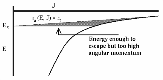
Figure 1: Schematic diagram of the energy–angular momentum plane for a star cluster. Using the energy criterion all stars with energy $E$ greater than the energy at the tidal radius $E_{\rm t}$ escape. If the apocenter criterion is applied paricles in the schaded region are not in an escape orbit and therefore remain bound to the cluster.

Figure 2: The total mass of the simulated clusters (normalized to the initial mass) as a function of time for different Fokker-Planck models in which the number of particles is $\infty$ (by definition).
The results of CW is presented as a $\bullet$ (to the left) at the mass and age of the system where they considered the cluster to cease to exist. The models in which the energy criterion is used are presented as the dashed line for the isotropic model Ie and the dotted line for the anisotropic model Ae.
The two lines to the right give the results of the anisotropic Fokker-Planck model in which the apocenter criterion is used (model Aa). The dash-dotted line uses the same stellar evolution model as is adopted by CW and for the solid line the stellar evolution program ${\sf SeBa}$ is used.
All runs were stopped at the points where the self-consistent potential could not be found.

Figure 3: Mass as a function of time for a number of Fokker-Planck models. The four solid lines represent the results of model Aa with 32k, 16k, 4k and 1k particles from left to right, respectively. Dotted curves present model Ie for the same numbers of particles as for model Aa.
The time scale for escapers via Eq. 1 with $\alpha_{\rm esc}=2$ for all models.

Figure 4: Mass as a function of time for the $N$-body models (dotted lines) and Fokker-Planck models Aa (solid lines, see also Figs. 2 and Fig. 3). The thick solid line to the left is for $\infty$ stars, the three subsequent solids are for 32k, 16k and 1k stars, respectively. The left and right thick dashed lines give the results of the $N$-body simulations for 32k and 16k stars, respectively. The two thin dashed lines represent the ${1\over 2}\sigma$ deviation from the mean of the 10 performed runs with 1k stars.
The results obtained by CW is presented as a $\bullet$.

References

- (1) Aarseth, S. J., Henon, M., Wielen, R. 1974, A&A, 37, 183
- (2) Chernoff, D., Weinberg, M. 1990, ApJ 351, 121
- (3) Cohn, H. 1979, ApJ 234, 1036
- (4) Fukushige, T., Heggie, D. C. 1995, MNRAS 276, 206
- (5) Giersz, M., & Heggie, D. C. 1994a, MNRAS 268, 257
- (6) Giersz, M., & Heggie, D. C. 1994b, MNRAS 270, 29
- (7) Heggie, D. C., Giersz, M., Spurzem, R., & Takahashi, K. 1998, To appear in Highlights of Astronomy Vol. 11, ed. Johannes Andersen, in press (astro-ph/9711191)
- (8) Hut, P. 1994, IAU 165, in Compact stars in binaries, eds. J. van Paradijs and E. P. J. van den Heuvel & E. Kuulkers, Kluwer, p. 377
- (9) Hut, P., Makino, J. & McMillan, S. 1995, ApJ 443, 93
- (10) Lee, H. M., & Ostriker, J. P. 1987, ApJ 322, 123
- (11) Makino, J., Aarseth, S. J. 1992, PASJ 44, 141
- (12) Makino, J., Taiji, M., Ebisuzaki, T., Sugimoto, D. 1997, ApJ 480, 432
- (13) Portegies Zwart, S. F., Verbunt, F. 1996, A&A 309 179
- (14) Portegies Zwart, S. F., & Yungelson, L. 1998, A&A 332, 173
- (15) Portegies Zwart, S. F., Tout, Ch. & Lee, M. H. 1998a, To appear in Highlights of Astronomy Vol. 11, ed. Johannes Andersen, in press (astro-ph/9710209)
- (16) Portegies Zwart, S. F., Hut, P., McMillan, S. L. W. & Makino, J. 1998b, A&A in press (astro-ph/9803084)
- (17) Spurzem, R. & Takahashi, K. 1995, MNRAS 272, 772
- (18) Takahashi, K. 1995, PASJ 47, 561
- (19) Takahashi, K. 1997, PASJ 49, 547
- (20) Takahashi, K., Lee, H. M., Inagaki, S. 1997, MNRAS 292, 331
- (21) Vesperini, E. & Heggie, D. C. 1997, MNRAS 289, 898