PROTOGALACTIC DISK MODELS OF DAMPED Ly$\alpha$ KINEMATICS

Abstract

We present new observational results on the kinematics of the damped Ly$\alpha$ systems. Our full sample is now comprised of 31 low-ion profiles and exhibits similar characteristics to the sample from Paper I. The primary exception is that the new distribution of velocity widths includes values out to a maximum of nearly 300 km s^-1 , $\approx$ 100 km s^-1 greater than the previous maximum. These high velocity width systems will significantly leverage models introduced to explain the damped Ly$\alpha$ systems. Comparing the characteristics from low-redshift and high-redshift sub-samples, we find no evidence for significant evolution in the kinematic properties of protogalaxies from $z=2.0-3.3$.

The new observations give greater statistical significance to the main conclusions of our first paper. In particular, those models inconsistent with the damped Ly$\alpha$ observations in Paper I are ruled out at even higher levels of confidence. At the same time, the observations are consistent with a population of rapidly rotating, thick disks (the TRD model) at high redshift, as predicted by cosmologies with early structure formation.

Buoyed by the success of the TRD model, we investigate it more closely by considering more realistic disk properties. Our goal is to demonstrate the statistical power of the damped Ly$\alpha$ observations by investigating the robustness of the TRD model. In particular, we study the effects of warping, realistic rotation curves, and photoionization on the kinematics of disks in the TRD model. The principal results are: (1) disk warping has only minimal effect on the kinematic results, primarily influencing the effective disk thickness, (2) the TRD model is robust to more realistic rotation curves; we point out, however, that the rotation curve derived from centrifugal equilibrium with HI gas alone does not yield acceptable results, rather flat rotation curves such as those generated by dark matter halos are required, and (3) the effects of photoionization require thicker disks to give consistent velocity width distributions.

1. INTRODUCTION

This paper marks the third in a series of papers on the kinematics of the damped Ly$\alpha$ protogalaxies. These HI gas layers observed along sightlines to distant QSO’s are widely believed to be the gaseous progenitors of modern galaxies (Wolfe (1995)). Hence an examination of damped systems at high redshift provides insight into the process of galaxy formation. For instance, identifying the physical nature of these systems may distinguish between the monolithic collapse model (Eggen, Lynden-Bell, & Sandage (1962)) and the hierarchical scenario favored by standard cosmogony. In our first paper (Prochaska & Wolfe 1997b , hereafter PW), we demonstrated that the kinematics of damped Ly$\alpha$ systems at high redshift are consistent with these systems being thick, rapidly rotating disks; it is a description not unlike that predicted by monolithic collapse formation scenarios. At the same time, we found damped Ly$\alpha$ systems cannot be simple exponential disks in a cluster normalized Standard Cold Dark Matter cosmology (e.g. Kauffmann (1996)). Subsequently, Jedamzik and Prochaska (1998) tightened this conclusion by considering a range of disk characteristics and CDM normalizations. They found that only a finely tuned disk model within the framework of CDM could be made marginally consistent with the damped Ly$\alpha$ observations. Recently, Haehnelt et al. (1997) have offered an alternative model for damped systems as gaseous protogalactic clumps undergoing infall within dark matter halos which may be consistent with the kinematic characteristics of the damped Ly$\alpha$ systems. Such a description lends itself naturally to the hierarchical cosmologies where merging plays a vital role. A future paper will address this model in greater detail. For the present work, we will focus on the interpretation of damped Ly$\alpha$ systems as thick rotating disks at high redshift.

In PW, we analyzed the low-ion profiles from 17 damped Ly$\alpha$ systems and compared their kinematic characteristics with those of simulated profiles derived from several physical models. Of the models tested, we found the thick rotating disk model to be the only model consistent with the observations. The basic assumptions of the model are a flat rotation curve and an exponential gas distribution, both chosen to roughly correspond with the observations of local spiral galaxies. In this paper we present low-ion profiles for 14 additional damped systems. Therefore, our full kinematic sample consists of 31 low-ion profiles. We interpret the sample with disk models containing more physically realistic characteristics, e.g. disk warping and photoionization. We have two primary goals in mind: (1) to test the robustness of the interpretation of damped Ly$\alpha$ systems as disks and (2) to determine the effects on our conclusions regarding the thickness and rotation speed of these disks.

In $\S 2$ we review the terminology and methodology introduced in PW. The new data are presented and tested against the models of PW in $\S 3$. We investigate the effects of more realistic disk properties in $\S 4$ and in $\S 5$ we present a summary.

2. A REVIEW

Our strategy is to compare the kinematic characteristics of low-ion profiles in damped Ly$\alpha$ systems with the simulated profiles derived from various physical models. In this manner, then, we investigate the agreement between the models and the damped systems. In this section we review the methodology and the thick rotating disk (TRD) model presented in PW.

To characterize the kinematics of the damped systems we focus on low-ion profiles such as SiII 1808. After normalizing them to unit continuum strength, we create a binned apparent optical depth array, $\bar{\tau}(v)$, where $\bar{\tau}(v)=<\ln[I_{c}/I(v)]>$, $I(v)$ is the intensity at velocity $v$, $I_{c}$ is the continuum intensity, and the average is taken over $\approx$ two resolution elements centered at $v$. We focus on $\bar{\tau}(v)$ rather than $I(v)$ to minimize the effects of saturation, and we smooth in optical depth to both limit the effects of Poisson noise and focus on features as opposed to individual components. Each profile is characterized by its signal-to-noise ratio (SNR), instrumental resolution, and peak optical depth ratio, $\bar{\tau}(v_{pk})/\sigma(\bar{\tau})$, with $v_{pk}$ the position of the maximum of $\bar{\tau}(v)$ in velocity space.

In PW, the only model considered which is consistent with the damped Ly$\alpha$ kinematic characteristics is the TRD model. For this model, we assume:

• An exponential gas distribution

  $$n(R,Z)=n_{0}\exp\left[\,-\,{R\over R_{d}}-{|Z|\over h}\,\right]\;\;\;,$$ (1)

  where $R$ and $Z$ are cylindrical radius and vertical displacement from midplane, $n_{0}$ is the central gas density, $R_{d}$ is the radial scale length, and $h$ is the vertical scale height. Note $n_{0}$ is related to the perpendicular column density at $R=0$ by $N_{\perp}(0)=2n_{0}h$.

• A flat rotation curve parameterized by the rotation speed, $v_{rot}$

• A random Gaussian velocity field parameterized by a 1-d velocity dispersion, $\sigma_{cc}$.

For the model systems considered here, we derive simulated profiles with identical SNR, instrumental resolution, and peak optical depth as the empirical data set. We employ the same Monte Carlo techniques as those used in $\S 3.2$ of PW. However, we now consider 31 damped Ly$\alpha$ systems which includes the 17 systems used in PW. To sufficiently sample the model distributions requires $\approx 10000$ sightlines, thus we perform 31 runs of 333 sightlines for every simulation. The SNR, $\bar{\tau}(v_{pk})/\sigma(\bar{\tau})$, and instrumental resolution of the simulated profiles for each set of 333 sightlines is varied accordingly.

We quantify the kinematic characteristics of the profiles with 4 test statistics:

• Velocity Interval Test – The width of the profiles in velocity space, $({f_{\rm\Delta v}})$ or $\Delta v$. Formally, we calculate the total optical depth, $\tau_{tot}$ of the profile in velocity space and define $\Delta v$ to be the velocity width encompassing $0.9\,\tau_{tot}$ by trimming $0.05\,\tau_{tot}$ off each edge of the profile.

• Mean-Median Test – Measures the asymmetry of the profile

  $$f_{mm}={|v_{mean}-v_{median}|\over({f_{\rm\Delta v}}/2)}\;\;\;.$$ (2)

• Edge-Leading Test – Designates how edge-leading the peak of the profile is

  $$f_{edg}={|v_{pk}-v_{mean}|\over({f_{\rm\Delta v}}/2)}\;\;\;.$$ (3)

• Two Peak Test – Designates how edge-leading the 2nd peak of the profile is

  $$f_{2pk}={\pm}\frac{|v_{2pk}-v_{mean}|}{({f_{\rm\Delta v}}/2)}\;\;\;.$$ (4)

In the above equations, $v_{pk}$ and $v_{2pk}$ indicate the position of the peak and second strongest peak of the $\bar{\tau}(v)$ profile, and $v_{mean}$ and $v_{median}$ are the mean and median of the $\bar{\tau}(v)$ profile. We perform the statistical tests on the damped Ly$\alpha$ and simulated profiles in the same manner and compare the resulting distributions with the two-sided Kolmogorov-Smirnov (KS) Test.

3. DAMPED LYA PROFILES

3.1. DATA SAMPLES AND SELECTION CRITERIA

The full kinematic data sample, designated Sample B, comprises 17 damped Ly$\alpha$ systems from PW (Sample A) and 14 new systems. Table 1 contains the journal of the 14 new observations. In Table 2 we list the following properties of the 14 new profiles: absorption redshift (column 2), log of ${N({\rm HI})}$ (column 3), Fe abundance, i.e., $\log({\rm Fe/H})-\log({\rm Fe/H})_{\odot}$ (column 4), Zn abundance (column 5), the low-ion transition (column 6), and $\bar{\tau}(v_{pk})/\sigma(\bar{\tau})$ (column 7). From each new damped Ly$\alpha$ system we select a low-ion transition satisfying strict selection criteria. However, in order to include the highest redshift systems, we relax some of the selection criteria established in PW. This is because (1) the data have poorer SNR and (2) the high $z$ systems have lower metallicity. Thus, even strong transitions (e.g. Fe II 1608) are difficult to measure; for

Table 1 QSO and Observational Data

QSO	Date	Exp	$z_{em}$	Res	SNR	Data
		(s)		(km/s)		set
Q0019$-$01	F96	35000	4.528	7.5	18	W
Q0347$-$38	F96	12600	3.23	7.5	33	W
Q0951$-$04	S97	30600	4.369	7.5	13	W
Q1005+36	S97	3600	3.17	7.5	12	W
Q1346$-$03	S97	31000	3.992	7.5	29	W
Q1759+40	F96	10400	3.05	6.6	33	W
Q2348$-$14	F96	9000	2.940	7.5	41	W
Q0930+28	S97	17000	3.436	6.6	26	SL
Q1104$-$18	S97	19500	2.32	6.6	40	SL
Q1850+40	S97	11880	2.120	6.6	16	SL
Q2233+13	S97	15000	3.274	6.6	16	SL
Q2343+34	S97	40000	2.58	6.6	35	SL
Q2344+12	S97	15000	2.763	6.6	29	SL

^aW - Data acquired by Wolfe & Prochaska

^bQSO coordinates kindly provided by Becker (1998)

^cSL - Data kindly provided by W. L. W. Sargent, Limin Lu, and collaborators

Table 2

Additional Sample of DLA Systems QSO $z_{abs}$ $\log[{N({\rm HI})}]$ [Fe/H] [Zn/H] Transition $\bar{\tau}(v_{pk}/\sigma_{\bar{\tau}})$ Q0019$-$01 3.439 20.9 $>-1.7$ N/A FeII 1608 Q0347$-$38 3.025 20.8 $-1.8$ N/A FeII 1608 33 Q0951$-$04A 3.859 20.6 $-2.04$ N/A SiII 1526 Q0951$-$04B 4.203 20.4 $-2.94$ N/A SiII 1190 10 Q1005+36 2.799 20.6 $-2.0$ N/A FeII 1608 13 Q1346$-$03 3.736 20.7 $<-1.7$ N/A SiII 1304 29 Q1759+40 2.625 20.8 $-1.27$ N/A SiII 1808 41 Q2348$-$14 2.279 20.6 $-2.35$ $<-1.19$ FeII 1608 40 Q0930+28 3.235 20.3 $-2.03$ N/A FeII 1608 31 Q1104$-$18 1.661 20.8 $-1.40$ $-0.865$ SiII 1808 44 Q1850+40 1.990 21.4 $-1.33$ $-0.70$ ZnII 2026 16 Q2233+13 3.149 20.0 $-1.5$ N/A FeII 1608 19 Q2343+34 2.430 20.3 $-1.20$ N/A SiII 1808 25 Q2344+12 2.538 20.4 $-2.0$ N/A AlII 1670 36

^aAll limits are 3$\sigma$ limits

^bProfile is saturated at the peak

Figure 1.— Velocity profiles of low-ion transitions for the 14 new damped Ly$\alpha$ systems. For each profile, $v=0$ km s^-1 corresponds to the redshift labeled in the plot.

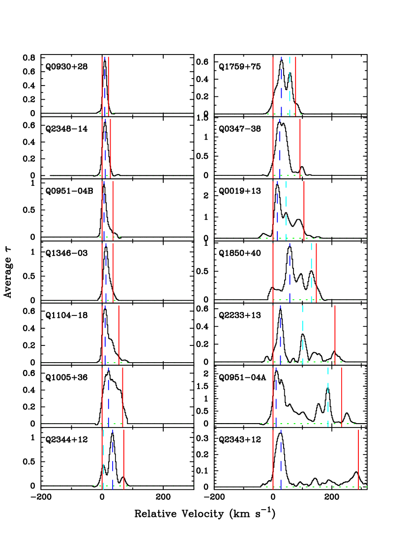
Figure 2.— Average optical depth profiles (binned over 9 pixels) for the 31 transitions comprising our new total empirical data set. The solid vertical lines designate the velocity interval, $\Delta v$, while the dash-dot lines indicate peaks and the dotted line is the $2\sigma(\bar{\tau})$ array. The profiles have been shifted in velocity space such that the left edge of the velocity interval coincides with $v=0$ and reflected in about half of the cases so that the strongest peak always lies on the left edge of the interval.

several of these damped systems no profile satisfies all the selection criteria of PW. Because we wish to maximize $\bar{\tau}(v)/\sigma(\bar{\tau})$ at the edge of each profile, in particular to ensure an accurate measurement of the velocity width, we adopt several profiles with peak normalized flux $I(v_{pk})/I_{c}<0.1$, which violates the previously established selection criterion (i.e. as in PW). In addition, we have relaxed the criterion that $\bar{\tau}(v_{pk})/\sigma(\bar{\tau})\geq 20$ on the grounds that numerical tests indicate this criterion was too conservative. In Figure 1 we present the velocity profiles as normalized intensity versus velocity, and the corresponding binned optical depth arrays in Figure 2. Note that many of the new profiles (e.g. Q0019$-$01, Q1104$-$18) exhibit the same edge-leading asymmetry characteristic observed for the profiles of Sample A. Furthermore, the distribution of profile widths resembles that of Sample A, but the new distribution extends to 290 km s^-1 which exceeds the 200 km s^-1 maximum width in Sample A. In fact, three of the 14 profiles have $\Delta v>200{\rm\;km\;s^{-1}}$. The incidence of $\Delta v>200{\rm\;km\;s^{-1}}$ in only one of 17 previous velocity profiles is due to small number statistics.

Figure 3.— Comparison of a mildly saturated low-ion profile with a weak profile for the damped Ly$\alpha$ systems toward (a) Q0019$-$01 at $z=3.439$ and (b) Q0951$-$04 at $z=3.859$. Note the profiles track one another very closely and therefore exhibit nearly the same kinematic characteristics, irrespective of the saturation.

Sample B includes two profiles with $I(v)/I_{c}<0.1$, including one with $I(v)/I_{c}<0.0$ where the flux falls below zero due to the effects of sky subtraction and Poisson noise. As emphasized in PW, the statistical tests used to characterize the profiles are sensitive to saturation; for example, a false determination of $v_{pk}$ leads to incorrect values for all 4 statistical tests. We have strong reason to believe, however, that we are not contaminating the results by including these two profiles. First, in each case the profile has $I(v)/I_{c}<0.1$ for only a few pixels. Therefore, the centroid of the peak is accurately determined to within a few km s^-1 . Secondly, we can compare the saturated profiles with weaker, noisier, profiles from the same damped system. In Figure 3, we show this comparison. Note that the profiles track one another very closely exhibiting nearly identical kinematic characteristics. Therefore, the kinematic results are not compromised by the minimal saturation evidenced in these two profiles. To calculate $\bar{\tau}(v)$ over the interval where $I(v)/I_{c}<0.0$ we arbitrarily set $I(v)/I_{c}=\sigma(I)/2$ and calculate $\bar{\tau}(v)$ accordingly. Having performed numerical experiments which demonstrate that the original criteria were too strict, we establish a new set of saturation criteria: (1) the line profile must be free of blending with other absorption line profiles, (2) the profile must not saturate for an excess of 1 resolution element, (3) the saturated region must not exceed one-fourth of the profile velocity width, (4) $\bar{\tau}(v_{pk})/\sigma(\bar{\tau})\geq 10$ instead of the previous value of 20. Together these criteria prevent an inaccurate determination of $v_{pk}$ and any resulting error in the test statistics.

To facilitate any parallel analysis performed with the damped Ly$\alpha$ surveys, where an accurate ${N({\rm HI})}$ is always measured (e.g. Wolfe et al. (1995)), and to allow for the most accurate comparison with the Monte Carlo simulations, we construct a subset of Sample B by imposing a stricter ${N({\rm HI})}$ criterion than that of PW. We refer to this subset of Sample B as Sample C. The criterion requires an ${N({\rm HI})}$ measurement for every damped system which must exceed $N_{thresh}=2{\rm\;\times\;10^{20}}\,{\rm cm^{-2}}$. This eliminates two systems from Sample A (Q1946$+$60A and Q0449$-$13) inferred to be damped Ly$\alpha$ systems on account of their large ionic column densities and one system (Q2212$-$16) with a measured ${N({\rm HI})}<N_{thresh}$. In addition, the criterion eliminates Q2233$+$13 from the new systems. Therefore, Sample C contains profiles from 27 damped systems. To investigate the evolution of the kinematic characteristics of the damped Ly$\alpha$ systems with redshift, we divide Sample C at its median redshift and consider two subsets: (i) a low redshift set of profiles with $\bar{z}=2.06$ and $z_{median}=1.96$ referred to as Sample D and (ii) a high redshift set of profiles with $\bar{z}=3.24$ and $z_{median}=3.35$ referred to as Sample E. Table 3 summarizes the 5 data samples.

Table 3

Data Samples Sample $N_{sys}$ Comment A 17 Original selection criteria B 31 New selection criteria C 27 ${N({\rm HI})}$ measurement required D 14 Low Redshift Cut of Sample C E 13 High Redshift Cut of Sample C

Figure 4 shows the statistical test distributions for Samples A$-$E. The results for Samples A and B are in good agreement indicating that the addition of the new systems will serve to strengthen the conclusions of PW. The only significant difference between the two samples is the tail observed out to nearly 300 km s^-1 in the ${f_{\rm\Delta v}}$ distribution of Sample B. One also notes Samples B and C exhibit nearly identical distributions, therefore the stricter ${N({\rm HI})}$ criterion has little effect on our results. Similarly, the only disagreement observed by eye between Samples D and E is in the Mean-Median Test, but statistically the two distributions are consistent ($P_{KS}=0.6$). We argue, therefore, that there is little evidence for an evolution of the kinematic characteristics with redshift. This will have significant impact on interpreting the damped Ly$\alpha$ systems in terms of the competing galaxy formation scenarios and will be further addressed in a future paper.

Figure 4.— Statistical test distributions for data Sample (A) the 17 damped Ly$\alpha$ profiles from PW, (B) the 31 profiles comprising the current data sample, (C) 27 of the current profiles which satisfy stricter ${N({\rm HI})}$ criteria, (D) a low redshift sub-sample and (E) a high redshift sub-sample.

3.2. ORIGINAL MODELS REVISITED

Figure 5 presents the statistical test distributions for Sample C as well as the distributions for 7 of the Monte Carlo models presented in PW. The $P_{KS}$ values are the KS Test probabilities that the model distribution and the corresponding distribution from Sample C could have been drawn from the same parent population. The TRD1 model is the ’best fit’ model to Sample A. For this model to $h/R_{d}=0.3$, $N_{\perp}(0)=10^{21.2}\,{\rm cm^{-2}}$ and $v_{rot}=225{\rm\;km\;s^{-1}}$, where $h$ is the vertical scale length, $R_{d}$ is the radial scale length, $N_{\perp}(0)$ is the central column density normal to the disk, and $v_{rot}$ is the flat rotation speed. The TRD2 model is identical to the TRD1 model except $v_{rot}=300{\rm\;km\;s^{-1}}$. The remaining models are identical to those from $\S 6$ of PW.

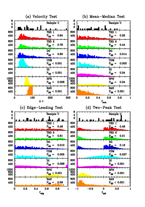
Figure 5.— The statistical test distributions for the models introduced in PW compared against Sample C. Note that all of the models which were ruled out in PW ($P_{KS}<5\%$) are ruled out at even higher confidence levels now.

The addition of the new profiles has tightened the primary results of PW in every case. In particular, we point out the continued failure of every model except the TRD model to reproduce the damped Ly$\alpha$ observations. The TRD1 model is generally consistent with Sample C, but because the model adopts the same rotation speed ($v_{rot}=225{\rm\;km\;s^{-1}}$) for all of the disks, it predicts no damped Ly$\alpha$ systems with velocity width $\Delta v>250{\rm\;km\;s^{-1}}$. Hence, this simple model cannot reproduce the high $\Delta v$ tail of the new empirical ${f_{\rm\Delta v}}$ distribution. By contrast, the distribution from the TRD2 model extends to $\Delta v\approx 300{\rm\;km\;s^{-1}}$ and therefore provides a better match to the high $\Delta v$ tail. Figure 6 plots the relative likelihood ratio test results for Sample C against the TRD model with the central HI column density (a) ${N({\rm HI})}=10^{20.8}\,{\rm cm^{-2}}$, (b) ${N({\rm HI})}=10^{21.2}\,{\rm cm^{-2}}$, and (c) ${N({\rm HI})}=10^{21.6}\,{\rm cm^{-2}}$. The figure indicates a lower limit of $v_{rot}>250{\rm\;km\;s^{-1}}$ and that the optimal rotation speed is $v_{rot}\approx 300{\rm\;km\;s^{-1}}$. However, if damped systems evolve to present galaxies, then a single population of disks with $v_{rot}=300{\rm\;km\;s^{-1}}$ is unacceptable as such large rotation speeds are rarely observed. One concludes the single population disk model is too simple and must be revised. Models including distributions of rotation speeds and sightline encounters with multiple disks will be considered in future papers. In this paper we retain the assumption of a single population of disks and study how more realistic disk properties affect the test statistic distributions.

Figure 6.— Isoprobability contours derived from the Likelihood Ratio Test for the TRD model against the $f_{\Delta}v$ distribution from Sample C with $N_{\perp}(0)=$ (a) $10^{20.8}\,{\rm cm^{2}}$, (b) $10^{21.2}\,{\rm cm^{2}}$, and (c) $10^{21.6}\,{\rm cm^{2}}$. Contour levels are drawn at $P$ = 0.01, 0.05 and 0.32. Note that the $f_{\Delta}v$ distribution would imply rotation speeds $v>250{\rm\;km\;s^{-1}}$ given the assumption of a single population of disks.

4. IMPROVED DISK MODELS

In this section we improve on the TRD model by introducing more realistic disk characteristics. We test the TRD model against the damped Ly$\alpha$ observations in the light of these properties and thereby gauge the robustness of the model. The discussion focuses primarily on the velocity width test statistic because the other test statistics are less sensitive to changes in disk properties.

4.1. THE WARPED DISK MODEL

HI 21 cm observations of local spiral galaxies (e.g. Briggs (1990)) suggest a significant fraction of disks are warped. Therefore, if the damped Ly$\alpha$ systems evolve into disk galaxies, as we have argued, the effects of warps must be considered. Warps produce two opposite kinematic effects: (i) some warped disks will have a large cross-section to sightlines which satisfy ${N({\rm HI})}\geq 2{\rm\;\times\;10^{20}}\,{\rm cm^{-2}}$ with large impact parameter and therefore small $\Delta v$. For instance, a tangent to the outer edge of a warped disk may have very large impact parameter (small $\Delta v$) yet still satisfy the ${N({\rm HI})}$ criterion (see Figure 9a below), and (ii) those sightlines which doubly penetrate the disk (at a warped edge in addition to the unwarped inner disk, see Figure 9b) will tend to yield larger $\Delta v$ than if they penetrated an unwarped disk. If the latter effect dominates, one expects a warped disk to yield a ${f_{\rm\Delta v}}$ distribution with a greater number of large $\Delta v$ values, which imitates a thicker and/or more rapidly rotating unwarped disk. In some cases, however, we find that the former effect dominates the results thereby lowering the median of the ${f_{\rm\Delta v}}$ distribution.

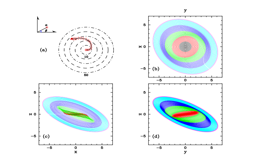
Figure 7.— The polar plot depicts the line of nodes for a warped disk. Each successive point on the solid line indicates rings of monotonically increasing radii. The azimuthal angle ($\beta$) indicates the rotation angle of the ring and the ‘radial’ angle ($\alpha$) designates the tilt angle of the ring. The remaining plots show the warped disk as a series of rings viewed from three perspectives.

Figure 8.— Lines of nodes for the four canonical warped disks: (a) an unwarped disk, (b) M33, (c) M83, and (d) an artificial warp. The polar plot has the same meaning as in Figure 7. The x-y plot reveals the radial dependence of the tilt angle as a function of the effective Holmberg Radius, $R_{H}$.

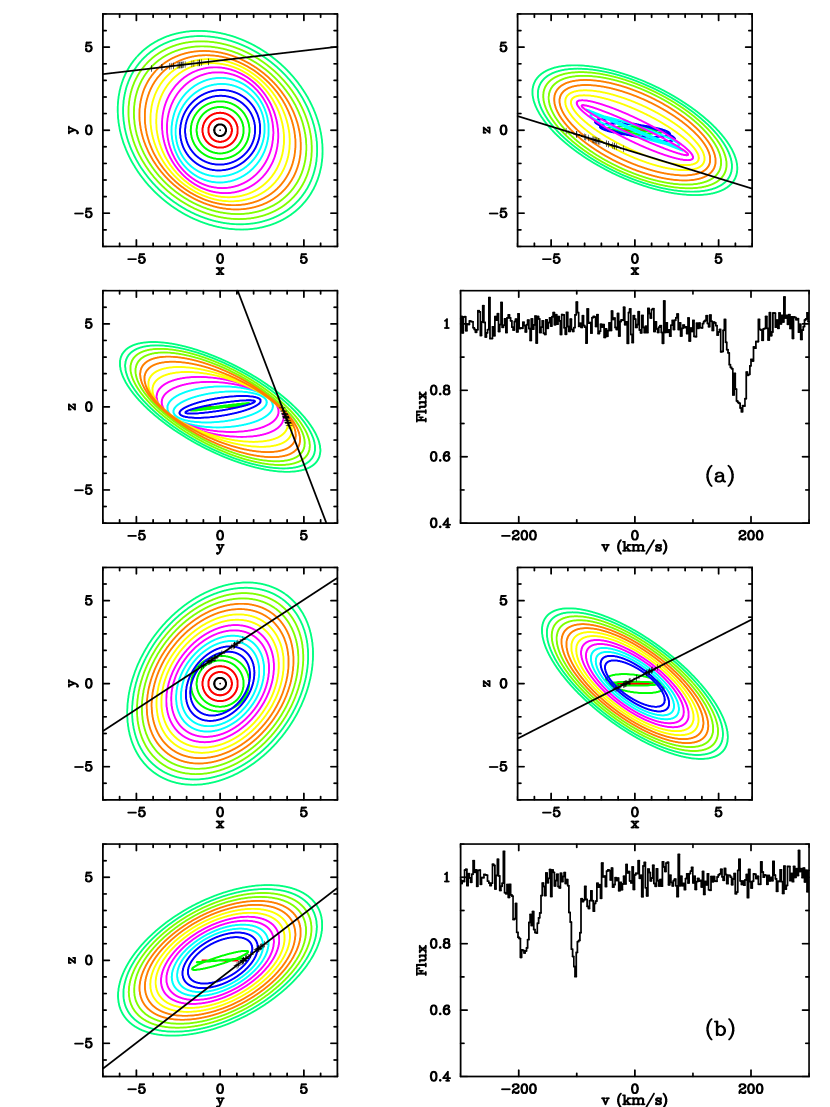
Figure 9.— Illustration of the two principal kinematic effects associated with warped disks: (a) a sightline with large impact parameter yielding a small $\Delta v$ which would not be included in a treatment of an unwarped disk as ${N({\rm HI})}$ would be less than $N_{thresh}$; (b) a sightline doubly penetrating the disk resulting in a significantly larger $\Delta v$ than if the disk were not warped. The + signs indicate the position of clouds along the sightline.

Unlike the TRD model, the warped disk model cannot be treated analytically. Standard modeling techniques involve decomposing the disk into a number of concentric rings, each with a unique orientation, with the configuration described by a ’line of nodes’. Figure 7a is a polar plot of a ’line of nodes’ where each successive point identifies rings with larger radii. We have used different symbols to help distinguish the points. The radial distance ($\alpha$) to each symbol indicates the tilt angle, and the azimuthal position ($\beta$) designates the position angle of the tilt axis. We define the reference plane by the orientation of the rings with smallest radius, i.e. the inner disk. Figures 7b-d show 3 views of the warped disk corresponding to this line of nodes. In the following, we consider 4 lines of nodes characterized by $R_{H}$, an effective Holmberg Radius, which sets the radial separation of the rings. Figure 8 plots the lines of nodes with respect to $R_{H}$. Included is a NULL line of nodes (Figure 8a) describing an unwarped disk, the lines of nodes for M83 and M33 (Figure 8b,c respectively; Briggs (1990)) and an artificially constructed line of nodes (CLON). Because we treat the warp model numerically, we will compare against the results of the null models and not the analytic TRD Model in order to properly measure the consequences of warping without being biased by any numerical effects. Figure 9 illustrates the two kinematic effects mentioned above. In Figure 9a a sightline penetrates a disk described by the WRP4 model and has a large impact parameter. The column density derived for this sightline is ${N({\rm HI})}=1.6{\rm\;\times\;10^{21}}\,{\rm cm^{-2}}$ and the resulting profile is plotted in the lower right panel. Note that this system would have ${N({\rm HI})}<2{\rm\;\times\;10^{20}}\,{\rm cm^{-2}}$ for all of the other lines of nodes considered here and would therefore not contribute to the test statistic distributions. The more common kinematic effect is illustrated in Figure 9b where we plot a sightline doubly penetrating a disk from the WRP2 model. The resulting profile is significantly wider than if the disk were not warped.

Table 4

Warp Parameters

Label	$h/R_{d}$	LON	$R_{H}/R_{d}$
WRP1	0.2	NULL	–
WRP2	0.2	M33	2.0
WRP3	0.2	CLON	2.0
WRP4	0.2	M83	2.0
WRP5	0.2	CLON	3.0
WRP6	0.3	NULL	–
WRP7	0.3	M83	2.0
WRP8	0.3	CLON	2.0

Figure 10.— The ${f_{\rm\Delta v}}$ distribution for 8 warp models compared against that for Sample C. The results demonstrate that warping has only a minor effect on the TRD Model.

We performed a series of Monte Carlo simulations for warped disks with a variety of thicknesses, $R_{H}/R_{d}$ values, and lines of nodes. Figure 10 plots the ${f_{\rm\Delta v}}$ distribution for 8 representative warp models corresponding to the parameters listed in Table 4. All of the models assume a rotation speed of $v_{rot}=250{\rm\;km\;s^{-1}}$ and a central column density, $N_{\perp}(0)=10^{21.2}\,{\rm cm^{-2}}$. In general, warping yields a greater number of moderate $\Delta v$ values ($\Delta v\approx{1\over 2}v_{rot}$) and a few more large $\Delta v$ values. This is the case for the M33 and CLON lines of nodes (e.g. compare the null model, WRP1, with WRP2 and WRP3) where the results resemble those for a thicker disk. This is not true for all lines of nodes. Note the difference between the results for models WRP3 and WRP4 which correspond to the CLON and M83 lines of nodes respectively. While both warps attain a tilt angle of $\approx 40^{\circ}$ at $R_{H}=2R_{d}$, the M83 warp has a much larger cross-section to sightlines satisfying the ${N({\rm HI})}$ criterion. As demonstrated in PW, those sightlines with large impact parameters tend to have smaller $\Delta v$, therefore the WRP4 model actually does more poorly than the unwarped disk, even though there are a number of sightlines which doubly penetrate the disk. The results are also sensitive to the adopted value of $R_{H}/R_{d}$. Comparing models WRP3 and WRP5 one notes the reduced effects of warping for larger $R_{H}/R_{d}$. As typical values of $R_{H}/R_{d}$ in local disks generally exceed 3, we expect warping to have even less of an effect on the ${f_{\rm\Delta v}}$ distribution than presented here. Curves WRP6$-$8 demonstrate the results for warping for thicker disks. Qualitatively, the changes in the ${f_{\rm\Delta v}}$ distribution are the same as those for the thinner disks.

To summarize, warping has only a moderate effect on the profile kinematics. For those lines of nodes where the dominant effect is of sightlines that penetrate the disk two times, warping mimics thicker disks, i.e. one observes a larger number of moderate $\Delta v$ values in the ${f_{\rm\Delta v}}$ distribution. Furthermore, warping can also lead to significantly fewer moderate $\Delta v$ values when the cross-section to damped Ly$\alpha$ system extends to higher impact parameter. This is the case for systems where the outer rings of the warp have $\beta\approx 180^{\circ}$. Having performed simulations for a large range of $h$, $R_{H}/R_{d}$, and lines of nodes, we quantify the results as follows: (1) in extreme cases, warping mimics disks with up to $50\%$ larger or smaller effective thickness ($h/R_{d}$ value), (2) warping lends to few additional large $\Delta v$ values in the ${f_{\rm\Delta v}}$ distribution and therefore has little effect on the acceptable values for $v_{rot}$, and (3) we find very thin ($h/R_{d}<0.1$) warped disks are inconsistent with the damped Ly$\alpha$ observations.

4.2. ROTATION CURVES

In PW, the velocity field of the exponential disk model was given by $v_{\phi}=v_{rot},v_{R}=v_{Z}=0$, i.e., we assumed a flat rotation curve independent of radius and height above the midplane of the disk. This is a good zeroth order representation for the rotation curve of spiral disks at large radii. But it breaks down at small radii because of the singularity implied for the mass density at $R=0$. In more realistic models the density approaches a finite central value at $R$ less then some core radius, resulting in $v_{\phi}=0$ at $R=0$. The independence of $v_{\phi}$ with $Z$ may also be unrealistic. In their analysis of the kinematics of the ionized gas associated with CIV absorption lines, Savage and Sembach (1995) find evidence that $v_{\phi}=v_{rot}$ up to $|Z|\approx 5$ kpc above midplane. On the other hand Sancisi (1998) finds evidence for a decrease in $v_{\phi}$ with increasing $|Z|$ in his HI studies of edge-on spirals. In fact, unless there is strong coupling between layers of adjacent $Z$ this is what one expects. Therefore, a more physical rotation curve will (i) approach $v_{rot}=0{\rm\;km\;s^{-1}}$ at $R=0$ where the enclosed mass density presumably approaches a finite value and (ii) likely decrease in speed with increasing height above the midplane. In this section, we consider a range of rotation curves appropriate for a system comprised of a thick disk, bulge, and dark matter halo.

4.2.1 Thick Disk

As demonstrated in PW (reaffirmed in $\S$3.2), the kinematics of the damped Ly$\alpha$ systems are consistent with thick rotating disks. Furthermore, we showed that the vertical scale height, $h$, must be greater than one-tenth the radial scale length, $R_{d}$. Therefore, the thin disk approximation is not applicable for deriving the rotation curve of these disks. In this section, we detail a numerical solution for the rotation curve of a thick disk by explicitly solving Poisson’s equation and combining the solution with the condition for centrifugal equilibrium.

The Fourier-Bessel Transformation Method

Our approach is an extension of the technique developed by Toomre (1963) for the thin disk solution and more recently applied by Casertano (1983) to the rotation curve for a thick disk at midplane. We calculate the disk potential by Fourier-Bessel transforming Poisson’s equation,

$$\nabla^{2}\Phi=4\pi G\rho\;\;\;.$$ (5)

We adopt an exponential mass density of the form,

$$\rho(R,Z)=\rho_{0}\exp(-R/R_{d})\exp(-|Z|/h)\;\;\;,$$ (6)

where $\rho_{0}$, the central mass density, is related to the central surface density, $\Sigma_{0}$, and central HI column density, $N_{\perp}(0)$, by

$$\rho_{0}={\Sigma_{0}\over 2h}=\mu m_{p}{N_{\perp}(0)\over 2h}\;\;\;,$$ (7)

with $\mu$ the molecular weight relative to Hydrogen. This relation implicitly assumes that the mass of the disk is dominated by HI gas, i.e., we ignore any contribution from stars or molecular Hydrogen.

Taking the Fourier-Bessel transformation of Poisson’s equation, we find

$$\tilde{\Phi}(k,Z)={-2\pi G\over k}\int\limits_{-\infty}^{+\infty}\exp(-k|Z-\zeta|)\,\tilde{\rho}(k,\zeta)\,d\zeta\;\;\;,$$ (8)

where

$$\tilde{\rho}(k,\zeta)=\rho_{0}\;\exp\left(\,{-|\zeta|\over h}\,\right)\times$$ (9)

$$\int\limits_{0}^{\infty}J_{0}(kR)\;\exp(-R/R_{d})\;R\;dR\;\;\;.$$

This integral is analytic (Gradshteyn & Ryzhik (1980), 6.623 [2]):

$$\tilde{\rho}(k,\zeta)={2\,R_{d}^{-1}\,\Gamma({3\over 2})\rho_{0}\over\sqrt{\pi}\,(R_{d}^{-2}+k^{2})^{3\over 2}}\;\exp\left(\,{-|\zeta|\over h}\,\right)\;\;\;.$$ (10)

Evaluating $\tilde{\Phi}(k,Z)$, we find

$$\tilde{\Phi}(k,Z)={A\over k\,(R_{d}^{-2}+k^{2})^{3\over 2}}\bigg{\{}{1\over hk+1}\big{[}\exp(-Z/h)$$ (11)

$$+\exp(-kZ)\big{]}\,+{1\over hk-1}\left[\,\exp(-Z/h)-\exp(-kZ)\,\right]\bigg{\}}\;\;\;.$$

where the constant $A$ is

$$A={G\,\pi\,\Sigma_{0}\over R_{d}}\;\;\;.$$ (12)

Finally, we take the inverse transform of $\tilde{\Phi}$,

$$\Phi(R,Z)=\int\limits_{0}^{\infty}J_{0}(kR)\;\tilde{\Phi}(k,Z)\;k\;dk\;\;\;.$$ (13)

The thick disk rotation curve is therefore given by,

$$v_{\phi}^{2}|_{\rm disk}(R,Z)=-R{\partial\over\partial R}\,\Phi(R,Z)$$ (14)

$$=R\int\limits_{0}^{\infty}J_{1}(kR)\,\tilde{\Phi}(k,Z)\,k^{2}\,dk\;\;\;,$$

which can be evaluated very accurately with standard numerical techniques. As the value for $\Sigma_{0}$ derived from the damped Ly$\alpha$ observations (i.e. $N_{\perp}(0)$) is significantly lower than that observed in present galaxies, the disk rotation curve will peak at $v_{max}\ll 200{\rm\;km\;s^{-1}}$ ($v_{\phi}^{2}\propto\Sigma_{0}R_{d}$) unless the HI gas contributes only a small fraction $(<30\%)$ of the disk mass. While it is possible that stars may double the surface density in the inner part of the disk (see Wolfe $\&$ Prochaska (1998)), we proceed under the assumption that the HI gas dominates.

Figure 11.— The rotation curve at midplane, $v_{circ}(R,0)$, for five disks with varying thickness, $h/R_{d}$. All of the curves are normalized to have the same central column density $N_{\perp}(0)$. There is only small dependence on thickness for the rotation curves.

Figure 12.— The rotation curves for a disk with $h/R_{d}=0.3$ at various heights within the disk.

Table 5Rotation Curves

Crv	$v_{disk}^{max}$	$\Sigma$	$v_{b}$	$R_{b}$	$v_{h}$	$R_{h}$	Comment
	(km/s)	$(M_{\odot}/{\rm pc^{2}})$	(km/s)	($R_{d})$	(km/s)	($R_{d})$
1	250	–	–	–	–	–	FLT
2	41	18	–	–	–	–	DLA disk
3	250	1450	–	–	–	–	Massive disk
4	250	18	–	–	250	0.5	DSK+HLO 1
5	250	18	–	–	250	5.0	DSK+HLO 2
6	250	18	180	0.1	250	0.5	DSK+HLO+BLG 1
7	250	18	180	0.1	250	5.0	DSK+HLO+BLG 2

Thick Disk Curves

Figure 11 shows the rotation curve at midplane, $v_{\phi}(R,0)$, derived from Equation 14 for 5 disks with varying thickness. Also plotted is the rotation curve derived with the thin disk approximation, normalized to have the same maximum rotation speed as the curve with $h/R_{d}=1{\rm\;\times\;10^{-5}}$. These two curves are in such close agreement that they are indistinguishable in Figure 11, verifying the accuracy of the numerical solution. Note all of the other curves are normalized to have the same central column density, $N_{\perp}(0)$. Physically this normalization implies very different central mass densities for the different thickness disks ($\rho_{0}\propto N_{\perp}(0)h^{-1}$). There is a decrease in $v_{\phi}$ with increasing $h/R_{d}$, as expected, because $\rho_{0}$ is smaller and therefore the centrifugal force is smaller at a given radius $R$. Even for $h/R_{d}=0.3$, however, the resulting rotation curve nearly traces that for the thin disk.

The rotation curve at various heights in a disk with $h/R_{d}=0.3$ is plotted in Figure 12. Note the curves at $Z=1.67\,h$ and at midplane differ by less than $10\%$, and even at $Z=6.67\,h$ there is generally less than a $50\%$ effect. We find similar results for disks of all thicknesses. Since nearly all of the gas arises within $\approx 2h$ of the midplane, in general we expect the decrease in $v_{\phi}$ with increasing $Z$ to have little effect on the kinematic results. In fact, it is possible the decrease in $v_{\phi}$ will actually increase the differential rotation along a given sightline.

4.2.2 Bulge and Halo

For the bulge rotation curve we assume the Hernquist Bulge model (Hernquist (1990)) parameterized by the peak velocity, $v_{b}$, and core radius, $R_{b}$

$$v_{circ}^{2}|_{\rm Bulge}(r)=4v_{b}^{2}{rR_{b}\over(r+R_{b})^{2}}\;\;\;,$$ (15)

where we can relate $v_{b}$ and $R_{b}$ to the bulge mass, $M_{b}$ by the following expression:

$$M_{b}=2.7{\rm\;\times\;10^{9}}M_{\odot}\;\left(\,{v_{b}\over 200{\rm\;km\;s^{-1}}}\,\right)^{2}\left(\,{R_{b}\over 100{\rm pc}}\,\right)\;\;\;.$$ (16)

Meanwhile, for the halo we require a density profile which yields a flat rotation curve at large radii. We adopt the following density profile,

$$\rho|_{\rm Halo}(r)={\rho_{h}\over 1+(r/R_{h})^{2}}\;\;\;,$$ (17)

where $\rho_{h}$ is the central density of the halo and $R_{h}$ is the core radius. This gives the following rotation curve,

$$v_{circ}^{2}|_{\rm Halo}(r)=v_{h}^{2}\left[\,1-{R_{h}\over r}\tan^{-1}\left(\,{r\over R_{h}}\,\right)\,\right]\;\;\;,$$ (18)

where $v_{h}$ is the halo rotation speed at large radii.

As both the bulge and halo are spherically symmetric, the rotation curves in cylindrical coordinates are:

$$v_{\phi}^{2}|_{\rm Bulge}(R,Z)={R^{2}\over\sqrt{R^{2}+Z^{2}}}{4v_{b}^{2}R_{b}\over(\sqrt{R^{2}+Z^{2}}+R_{b})^{2}}$$ (19)

and

$$v_{\phi}^{2}|_{\rm Halo}(R,Z)=v_{h}^{2}{R^{2}\over R^{2}+Z^{2}}\Bigg{[}1-$$ (20)

$${R_{h}\over\sqrt{R^{2}+Z^{2}}}\tan^{-1}\left(\,{\sqrt{R^{2}+Z^{2}}\over R_{h}}\,\right)\Bigg{]}\;\;\;.$$

Figure 13.— The left hand side plots the rotation curve at midplane for disks with varying bulge, halo, and disk components. The right hand side plots the ${f_{\rm\Delta v}}$ distributions for the 8 curves compared against Sample C.

4.2.3 Results

The disk rotation curve is uniquely parameterized by $h$ and $\Sigma_{0}$, where $h$ and all other distance scales are in units of the radial scale length, $R_{d}$, and $\Sigma_{0}$ is the disk surface density at $R=0$. The bulge and halo models are each parameterized by two variables which describe the slope of the curve ($R_{b},R_{h}$) and the maximum rotation speed ($v_{b},v_{h}$) at $Z=0$. The total rotation speed, then, is given by

$$v_{\phi}^{2}|_{\rm Tot}(R,Z)=v_{\phi}^{2}|_{\rm Halo}(R,Z)\;+\;v_{\phi}^{2}|_{\rm Bulge}(R,Z)$$ (21)

$$+v_{\phi}^{2}|_{\rm Disk}(R,Z)\;\;\;.$$

We have performed simulations for a wide range of the six parameters. The main results of the analysis are presented in Figure 13 and the rotational parameters are given in Table 5. Also listed is the peak rotation speed of each rotation curve, $v_{max}$. For all of the models presented here, we assume $N_{\perp}(0)=10^{21.2}\,{\rm cm^{-2}}$ and that $h/R_{d}=0.3$.

To facilitate a direct comparison with the TRD model, we plot the results for a flat rotation curve with $v_{max}=250{\rm\;km\;s^{-1}}$. For a given value of $v_{max}$, the flat rotation curve yields a greater fraction of large velocity widths than any other rotation curve. Therefore, it gives the best agreement with the empirical distribution provided $v_{max}\lesssim 350{\rm\;km\;s^{-1}}$, above which the distribution has too many large $\Delta v$ values. For model CRV2, we assume a thick disk with $\Sigma_{0}=\mu m_{p}N_{\perp}(0)=18M_{\odot}/{\rm pc^{2}}$ and $R_{d}=10$ kpc which implies $v_{max}=41{\rm\;km\;s^{-1}}$. This model corresponds to $N_{\perp}(0)=10^{21}\,{\rm cm^{-2}}$ as inferred from the damped Ly$\alpha$ observations. The value of $R_{d}$ was chosen to roughly correspond to the cross-section derived for damped Ly$\alpha$ systems assuming a number density approximately equal to that for spiral galaxies in the present epoch (Wolfe et al. (1995)). As noted above and shown in Figure 13, the mass associated with the HI disk implies a rotation curve which is inconsistent with the damped Ly$\alpha$ observations. The results for the CRV3 model demonstrate that a disk with $\Sigma_{0}=1440M_{\odot}/{\rm pc^{2}}$ and $R_{d}=5\;\rm kpc$ is consistent, yet this implies that $>95\%$ of the disk mass is in a component other than HI gas. It is unlikely that $\Sigma_{0}$ approaches even $500M_{\odot}/{\rm pc^{2}}$ given current estimates of the stellar (Wolfe $\&$ Prochaska (1998)) and molecular (Ge & Bechtold (1997)) baryonic fraction. Furthermore, if $\Sigma_{0}\approx 1500M_{\odot}/{\rm pc^{2}}$ in every damped system, this would imply a comoving density approximately 100 times that of visible matter in the present universe. On the other hand if we include a massive dark halo ($v_{h}=250{\rm\;km\;s^{-1}})$, the resulting ${f_{\rm\Delta v}}$ distribution (CRV4) is consistent with the empirical distribution provided $R_{h}/R_{d}\lesssim 1$. For larger values of $R_{h}/R_{d}$, the rotation curve (CRV5) rises too slowly to yield large $\Delta v$. Finally, we investigate the effect of including a massive bulge in models CRV6 and CRV7 where we adopt the same disk and halo curves from models CRV4 and CRV5. We find the presence of a massive bulge $(v_{b}=180{\rm\;km\;s^{-1}}$) with $R_{b}\ll R_{d}$ has little impact on the ${f_{\rm\Delta v}}$ distribution as the bulge affects only the inner rotation curve. To conclude, the TRD model requires a rotation curve which is nearly flat for $R_{d}>1$. While this can be achieved with a massive disk resembling that of the Milky Way, it would requires a non-gaseous baryonic component with comoving density two orders of magnitude greater than the density of visible matter in current galaxies, which is implausible. Assuming that the mass of the disk is dominated by the HI gas with $N_{\perp}(0)\approx 10^{21}\,{\rm cm^{-2}}$ requires the presence of a massive dark halo with $R_{h}\lesssim R_{d}$.

4.3. PHOTOIONIZATION

Over the redshift range spanning our damped Ly$\alpha$ observations the IGM is primarily ionized, presumably by the ambient UV radiation field from background quasars. At redshift $z\sim 2.5$ the UV intensity is often described as a modified power law (Haardt & Madau (1996))

$$J(\nu)\approx J_{912}\left(\,{\nu\over\nu_{912}}\,\right)^{\alpha}$$ (22)

with $J_{912}\approx 10^{-21.5}\,{\rm erg/s\;s^{-1}\;cm^{-2}\;sr^{-1}\;Hz^{-1}}$ and exponent $\alpha\approx-1$. This background flux creates ionization fronts in the HI disks comprising the TRD Model, analogous to those observed in present spiral galaxies (Maloney (1993)). Because a complete treatment involving a solution of the radiative transfer equation is beyond the scope of this paper, we address the problem with two different approximations. In one case, we assume a sharp HI edge to the disks of the TRD model. In the other, we assume the gas is photoionized if its volume density is below some critical value. The photoionization of the disk will eliminate from the derived statistical sample those sightlines with ${N({\rm HI})}\approx N_{thresh}$. Since these sightlines tend to penetrate the disk at large impact parameters which yield small $\Delta v$, we predict a general shift in the ${f_{\rm\Delta v}}$ distribution to larger velocity widths. By analogy to the results from warped disk models, we expect the photoionized disk to mimic thicker disks.

First, we consider the HI Edge Model, which incorporates a sharp “HI edge” for the exponential disk at a column density, $N_{ph}$. Using a 2D analogy to the Str$\rm\ddot{o}$mgren sphere argument, we find that the column density of ionized gas above the HI gas is given by

$$N_{ph}={2\phi\over\alpha_{rec}<n>}\;\;\;,$$ (23)

where $\phi$ is the flux of ionizing photons

(i.e. $\phi=\int\limits_{\nu_{H}}^{\infty}d\nu\,2\pi J_{\nu}/h\nu$), $<n>$ is the average hydrogen volume density, and $\alpha_{rec}$ is the Case B recombination coefficient. Given the above value for $J_{912}$, with $<n>\,=1\,{\rm cm^{-3}}$ we find $N_{ph}\approx 10^{18}\,{\rm cm^{-2}}$. To simulate photoionization of the HI disks in the TRD model, we systematically remove $N_{ph}$ of column normal to the disk everywhere. This leads to a sharp HI edge at $R_{ph}=\ln[N_{\perp}(0)/2N_{ph}]$ and effectively removes $2N_{ph}$ from each sightline which penetrates within $R_{ph}$. As $J_{912}$ is poorly constrained observationally, we consider $J_{912}$ values ranging from $10^{-21.0}-10^{-22.5}\,{\rm erg\;s^{-1}\;cm^{-2}\;sr^{-1}\;Hz^{-1}}$, where the favored value is $10^{-21.5}$ (Haardt & Madau (1996)). To consider meaningful $N_{ph}$ values, we relate $N_{ph}$ to $N_{\perp}(0)$, $h$, and $J_{912}$ with the following equation:

$$N_{ph}=10^{19}\,{\rm cm^{-2}}\left(\,{h/R_{d}\over 0.2}\,\right)\left(\,{J_{912}\over 10^{-21.5}}\,\right)\left(\,{10^{21.2}\over N_{\perp}(0)}\,\right)\;\;\;.$$ (24)

The other approximation we make to describe the photoionization of the disk is to assume the gas is predominantly ionized below a critical volume density, $n_{ph}$. For the TRD model, the critical density can be defined as

$$n_{ph}=n(R=R_{ph},Z=0)={N_{ph}\over h}$$ (25)

with $R_{ph}$ and $N_{ph}$ defined as above. With $h=0.3R_{d}$, $R_{d}=5$ kpc, and $N_{ph}=10^{18}-10^{20}\,{\rm cm^{-2}}$ this implies density cutoffs of $n_{ph}\approx[10^{-4}-10^{-2}\,{\rm cm^{-3}}]$. We refer to this photoionization model as the Critical Density model.

Figure 14.— Test statistic distributions for the removed sightlines from four representative runs of the two photoionization models considered in the text.

Table 6

Photoionization Models Label Model $h/R_{d}$ $\log[{N({\rm HI})}]$ $-\log[J_{912}]$ $\log[N_{ph}]$ PHT 1 HI 0.3 21.2 22.0 18.7 PHT 2 HI 0.3 21.2 20.5 20.2 PHT 3 HI 0.3 20.8 21.5 19.6 PHT 4 HI 0.1 21.2 21.0 19.2 PHT 5 CD 0.3 21.2 22.0 18.7 PHT 6 CD 0.3 21.2 20.5 20.2 PHT 7 CD 0.3 20.8 21.5 19.6 PHT 8 CD 0.1 21.2 21.0 19.2

It is revealing to examine the kinematic characteristics of those sightlines removed from the TRD statistical sample on account of photoionization. Figure 14 plots the test statistics for the eliminated sightlines from 4 representative runs of each photoionization model the parameters of which are given in Table 6. Included in each panel of the ${f_{\rm\Delta v}}$ distribution is the percentage of sightlines eliminated. Note that very few sightlines are removed in a 10000 sightline run for $N_{ph}\approx 10^{18}\,{\rm cm^{-2}}$, hence the effects of photoionization are minimal for small $J_{912}$, larger $N_{\perp}(0)$ or small $h/R_{d}$. By contrast, simulations with $N_{ph}=10^{20}\,{\rm cm^{-2}}$ have very many sightlines removed so that there is a large impact on the simulations. As expected, the vast majority of sightlines eliminated have small $\Delta v$ and correspondingly small ${f_{\rm mm}}$ and ${f_{\rm 2pk}}$ values. Also, the results for thin disks are essentially unaffected by photoionization as most sightlines yield small $\Delta v$ irrespective of photoionization. The results are very similar for the two photoionization models, although the Critical Density model does remove a few more large $\Delta v$.

Figure 15.— Isoprobability contours for disks with (a) $N_{\perp}(0)=10^{20.8}\,{\rm cm^{-2}}$, (b) $N_{\perp}(0)=10^{21.2}\,{\rm cm^{-2}}$, and (c) $N_{\perp}(0)=10^{21.6}\,{\rm cm^{-2}}$, for a range of $h/R_{d}$ and $J_{912}$ values in the HI Edge Model.

Figure 16.— Plots of the ${N({\rm HI})}$ vs. $\Delta v$ pairs for the damped Ly$\alpha$ systems (boxes) and four photoionization models: PHT1 and PHT5 where $J_{912}$ is small and PHT2 and PHT6 where photoionization is significant. The $P_{KS}$ are derived from the 2-dimensional KS Test. Note that photoionization clearly worsens the agreement between the model and the empirical distribution.

The results presented in Figure 14 suggest photoionization will improve the agreement between models with small thickness or low rotation speed (i.e. models with an ${f_{\rm\Delta v}}$ distribution dominated by small $\Delta v$) and the empirical data set. However, besides eliminating sightlines with small ${N({\rm HI})}$, photoionization of the edges of the disks tends to lower the average $\Delta v$ for a given sightline; because of photoionization, the HI path along a given sightline is reduced, which reduces the differential velocity along the line of sight and on average lowers $\Delta v$. The net result is that photoionization actually worsens the agreement for disks of all thickness and central column density, contrary to our initial expectation. Figure 15 presents isoprobability $P_{KS}(\Delta v)$ contours for disks with (i) $N_{\perp}(0)=10^{20.8}\,{\rm cm^{-2}}$, (ii) $N_{\perp}(0)=10^{21.2}\,{\rm cm^{-2}}$, and (iii) $N_{\perp}(0)=10^{21.6}\,{\rm cm^{-2}}$, for a range of $h/R_{d}$ and $J_{912}$ values in the (a) HI Edge model and (b) Critical Density model. The three contours correspond to $P_{KS}(\Delta v)$ values of 0.01, 0.05, and 0.32 and the $\times$ marks the highest $P_{KS}(\Delta v)$ value in the explored parameter space. The agreement clearly worsens for increasing $J_{912}$ and decreasing $h/R_{d}$. If the UV background does have $J_{912}\approx 10^{-21}$, then photoionization will have a significant impact on the results derived for in the TRD Model. In particular, the thickness would have to exceed $h/R_{d}>0.2$ for disks with $N_{\perp}(0)=10^{20.8}\,{\rm cm^{-2}}$ and 0.3 for disks with larger $N_{\perp}(0)$. While such large values for $J_{912}$ are unlikely, they are not ruled out by current observations. For the $J_{912}\approx 10^{-21.5}$ the effect on the TRD model is moderate, generally requiring less than a $30\%$ increase in the thickness of the disks.

Lastly, we examine how the photoionization models affect the distribution of ${N({\rm HI})}$, $\Delta v$ pairs. In PW (Figure 13) we noted the rather poor concordance between the TRD model and the damped Ly$\alpha$ observations and suggested photoionization may improve the agreement. Specifically, we expected photoionization to reduce the number of sightlines with small $\Delta v$ and small ${N({\rm HI})}$ and thereby improve the agreement with the damped Ly$\alpha$ observations. Figure 16 plots the ${N({\rm HI})}$, $\Delta v$ pairs from Sample C (big squares) and the ${N({\rm HI})}$, $\Delta v$ pairs for 4 of the photoionization models. The PHT1 and PHT5 models indicate the results without significant photoionization while the PHT2 and PHT6 models highlight its effects. The $P_{KS}$ values were derived from the 2-dimensional Kolmogorov-Smirnov test (Press (1992)). For the reasons discussed above, photoionization worsens the agreement between the TRD model and damped distributions. While models PHT2 and PHT6 are inconsistent at the 99$\%$ c.l., it should be noted, however, that one can improve the concordance by considering a range of $v_{rot}$ and $N_{\perp}(0)$ values. Also, as noted in Wolfe & Prochaska (1998), the presence of many large $\Delta v$, small ${N({\rm HI})}$ pairs may indicate the presence of a ’hole’ in the inner region of the disk as observed in many local spirals.

5. SUMMARY AND CONCLUSIONS

We have presented new observations on the low-ion kinematics of the damped Ly$\alpha$ systems. The full sample of 31 profiles confirms the primary conclusions of PW, in particular, (i) models with kinematics dominated by random or symmetric velocity fields are inconsistent with the damped Ly$\alpha$ kinematics, (ii) the TRD model, which consists of a population of thick, rapidly rotating disks at high $z$, naturally reproduces both the observed edge-leading asymmetry of the empirical profiles as well as the distribution of velocity widths, and (iii) models incorporating centrifugally supported disks within the framework of the standard CDM cosmology are ruled out at high levels of confidence. In addition, a comparison of the kinematic properties of profiles of the highest redshift systems ($\bar{z}=3.24$) with the lower redshift systems ($\bar{z}=2.06$) reveals no significant evolution in the kinematics of the damped Ly$\alpha$ systems. This last observation may place strong constraints on scenarios of galaxy formation which predict significant evolution over this epoch.

Presently there are two working models which explain the kinematic characteristics of the damped Ly$\alpha$ systems: (1) the TRD model and (2) merging protogalactic clumps in numerical simulations of the standard Cold Dark Matter cosmology (Haehnelt et al. (1997)). In this paper we have focused on the TRD model. In particular, we have investigated the robustness of the model to including more realistic disk properties, specifically disk warping, physical rotation curves and photoionization. Given the prevalence of warping in local disk galaxies, we considered its effects on the kinematics of the disks in the TRD model. We found that the results of warping are dominated by two competing effects. Sightlines which penetrate both the unwarped inner disk and the warped outer disk yield moderately higher $\Delta v$ than those simply intersecting an unwarped disk. At the same time, however, some warped disks have significantly larger cross-section to sightlines with large impact parameters which tend to yield small $\Delta v$. Having considered a number of warped disks with a broad range of properties, we find: (i) in extreme cases, warping mimics disks with up to $50\%$ larger or smaller effective thickness ($h/R_{d}$ value), (ii) warping leads to very few extra large $\Delta v$ values in the ${f_{\rm\Delta v}}$ distribution and therefore has little consequence on the acceptable values for $v_{rot}$, and (iii) the lower limit to $h/R_{d}$ is nearly unchanged as we find $h$ must be $>0.1R_{d}$ for both warped and unwarped disks.

In PW, we assumed a flat rotation curve, $v_{\phi}=v_{rot}$, extending from $R=0\to\infty$ and $Z=0\to\infty$. In this paper we adopted rotation curves derived from specific bulge, halo, and disk components. Assuming an exponential profile is a good description of the density profile for the damped Ly$\alpha$ systems, we find the rotation curves derived from gravity generated by the HI gas alone cannot reproduce the empirical ${f_{\rm\Delta v}}$ distribution. If the rotation curve is dominated by the disk, one must introduce another mass component (e.g. stars, molecules) to establish consistency. At the same time we find that the rotation curve derived from a massive halo with core radius $R_{h}\lesssim R_{d}$ also yields a ${f_{\rm\Delta v}}$ distribution consistent with the observations. We believe that this latter explanation is more plausible. We also find the presence of the bulge to be largely inconsequential.

Lastly, we studied the effects of the intergalactic photoionizing background radiation on the disk kinematics. We made two separate approximations to model the photoionization of the disks: (a) an HI edge model where the disk is photoionized at radii $R>R_{ph}$ with $R_{ph}$ set by the intensity of the photoionizing background and the disk properties and (b) a Critical Density model where all gas with volume density $n\leq n_{ph}$ is presumed ionized. Contrary to our expectations, we find that photoionization tends to worsen the agreement between the TRD model and the damped Ly$\alpha$ observations. The effect, however, is not large ($<30\%$) for the favored value of $J_{912}=10^{-21.5}$, but for $J_{912}=10^{-21}$ a substantial $(>50\%)$ increase in the thickness of the disks would be required.

In summation, then, we find the TRD model is very robust to tests against the damped Ly$\alpha$ observations. The challenge remains, however, to consistently incorporate this model within a cosmological framework. While the clump model fits naturally within the SCDM cosmology, it must be demonstrated that the clump model exhibits similar robustness to comparisons with the damped Ly$\alpha$ kinematics. While Haehnelt et al. (1997) did show that the clump model could explain the damped Ly$\alpha$ observations from PW for a single set of parameters, a formal investigation of the full physical parameter space with meaningful statistics has yet to be performed. In addition, it is not clear how that model will change given different cosmological parameters, e.g. an Open Universe where merging plays a smaller role at $z\approx 2.5$. The model must also be tested against the new observations, in particular the new ${f_{\rm\Delta v}}$ distribution which extends to $\approx 300{\rm\;km\;s^{-1}}$. Finally, the fact that the numerical simulations do not reproduce the observed properties of modern galaxies when evolved to the present universe (Navarro, Frenk & White (1995)) suggests the model may have serious inconsistencies in the early universe.

In future papers we will introduce observations of the high-ion transitions (e.g. CIV 1548) with the aim of further constraining the two working models as well as advancing our understanding of the ionized gas associated with the damped Ly$\alpha$ systems. This gas is presumed to reside in the halo of these protogalaxies and therefore may give more direct indications of the dark matter associated with the damped Ly$\alpha$ systems. We also intend to consider effects (e.g. multiple disks) which would improve the agreement between the semi-analytic models of standard cosmology (Kauffmann (1996); Mo, Mao, & White (1997)).

References

- Becker (1998) Becker, R.H., private communication
- Binney and Tremaine (1987) Binney, J. and Tremaine, S. 1987, Galactic Dynamics (Princeton: Princeton University Press), p. 229
- Briggs (1990) Briggs, F.H. 1990, ApJ, 352, 15
- Casertano (1983) Casertano, S. 1983, MNRAS, 203, 735
- Eggen, Lynden-Bell, & Sandage (1962) Eggen, O.J., Lynden-Bell, D. & Sandage, A. 1962, ApJ, 136, 748
- Ge & Bechtold (1997) Ge, J. & Bechtold, J. 1997, ApJ, 477, 73
- Gradshteyn & Ryzhik (1980) Gradshteyn, I.S., & Ryzhik, I.M. 1980. Tables of Integrals, Series and Products. New York: Academic
- Haardt & Madau (1996) Haardt, F. & Madau, P. 1996, ApJ, 461, 20
- Haehnelt et al. (1997) Haehnelt, M.G., Steinmetz, M. & Rauch, M. 1997, astro-ph 9706201
- Hernquist (1990) Hernquist, L. 1990, ApJ, 356, 359
- Jedamzik & Prochaska (1998) Jedamzik, K. & Prochaska, J. X. 1998, MNRAS, in press (astro-ph 9706290)
- Kauffmann (1996) Kauffmann, G. 1996, MNRAS, 281, 475
- Maloney (1993) Maloney, P. 1993, ApJ, 414, 41
- Mo, Mao, & White (1997) Mo, H.J., Mao, S., & White, S.D.M. 1997, astro-ph/9707093
- Navarro, Frenk & White (1995) Navarro, J.F., Frenk, C.S., & White, S.D.M. 1995, MNRAS, 275, 56
- Press (1992) Press, W. H. 1992, Numerical Recipes in FORTRAN, (New York: Cambridge University Press)
- (17) Prochaska, J. X. & Wolfe, A. M. 1997, ApJ, 486, 73
- Sancisi (1998) Sancisi, R. 1998, private comm.
- Wolfe et al. (1995) Wolfe, A. M., Lanzetta, K. M., Foltz, C. B., and Chaffee, F. H. 1995, ApJ, 454, 698
- Wolfe (1995) Wolfe, A.M. 1995, in ESO Workshop on QSO Absorption Lines, ed. G. Meylan, (Berlin:Springer-Verlag), p. 13
- Wolfe Prochaska (1998) Wolfe, A.M. Prochaska, J. X., ApJ, 494, 15L